Modelling and correcting azimuthal anisotropy in Sentinel-1 backscatter data

ABSTRACT

Sentinel-1 backscatter data – acquired in dual-polarized (VV/VH) Interferometric Wide (IW) swath mode – show an azimuth angle dependency. The orientation of the tangential plane of the surface observed can alter the backscatter differently depending on the azimuth angle of the viewing geometry. In this study, two years of Sentinel-1 backscatter data over Western Europe have been investigated to show that the azimuthal anisotropy of backscatter is mainly caused by the orientation of the topography’s slope. The SRTM-3 digital elevation model (DEM) is used to describe the azimuthal anisotropy in the Tyrolean Alps and in addition, an algorithm is presented to take into account the azimuthal dependency by calculating correction parameters for each relative orbit of Sentinel-1.

1. Introduction

The Sentinel-1 mission is a C-band synthetic aperture radar (SAR) mission, which started in 2014. It is a constellation of two satellites orbiting the earth and has been developed and operated by the European Space Agency (ESA) within the Copernicus program. One of its acquisition modes is to sense the earth in Interferometric Wide Swath (IW). This is the main operational mode over land because it satisfies most service requirements, having a spatial resolution of about 20m and covering a swath area of 250km (European Space Agency (ESA) 2013). Information about the soil’s dielectric properties, the surface roughness or vegetation can be retrieved when another dependency of the backscatter is considered first: The backscatter coefficient changes with changing viewing geometry. Gauthier, Bernier, and Fortin (1998) highlighted this effect, noting that one should be aware of the incidence angle sensitivity before interpreting the temporal variability of the signal. Therefore, this geometric dependency of the radar beam has to be accounted for before information about e.g. surface soil moisture can be achieved. The geometry of the incidence radar beam can be described with an incidence (vertical) angle and an azimuth (horizontal) angle. In scatterometer missions, effects due to different azimuth angles were observed in time series over many geographical regions. These studies especially focused on either snow and ice masses (Early and Long 1997; Long and Drinkwater 2000; Fraser, Young, and Adams 2014) or sandy desert areas (Stephen and Long 2002; Stephen and Long 2003).

Bartalis, Scipal, and Wagner (2006) investigated the azimuthal anisotropy of scatterometer backscatter measurements over all global land areas and localized regions which show a strong azimuthal dependency. Problems which were explained by azimuthal effects were also identified by Envisat ASAR (Advanced Synthetic Aperture Radar) GM (global monitoring) backscatter time series over arid regions (Dostálová et al. 2014). In such areas, the ASAR backscatter from the descending and ascending orbits revealed a difference that adds a systematic bias in time series. This anisotropy has not been studied in more detail for Envisat ASAR and was either neglected or only partly considered when calculating backscatter model parameters and products separately for ascending and descending passes (e.g. Schlaffer et al. (2017)). For Sentinel-1 SAR data, Sabel et al. (2012) mentioned that azimuthal anisotropy causes additional discrepancies in the Sentinel-1 time series. Therefore, analysing the azimuthal anisotropy for Sentinel-1 SAR data is important from both a practical and a theoretical perspective.

In this paper, azimuthal effects in Sentinel-1 SAR backscatter data are investigated on a 1km scale. There are two reasons for this: Firstly, we would like to understand the dominant physical effects, disregarding small-scale effects like scattering reflecting from buildings. Secondly, Sentinel-1 data is usually terrain corrected with the freely available 3arcsec (approximately 90m) resolution SRTM-3 digital elevation model (DEM). With this coarse resolution, compared to the Sentinel-1 data, it would not be possible to characterize the target specific azimuthal modulation. Therefore, taking into consideration the Nyquist theorem, the 20m Sentinel-1 SAR data is down-sampled to a 500m grid, which is equivalent to 1km spatial resolution. Additionally, on this scale several products are achieved from Sentinel-1 data, e.g. surface soil moisture.

This paper has two objectives: The first objective is to study where azimuthal anisotropy occurs. Our hypothesis is that at the 1km scale, topography is the main reason for azimuthal effects. The second objective is to propose a possible solution to correct discrepancies due to the azimuthal anisotropy with a future prospect of improving product generation.

2. Azimuthal anisotropy

2.1. Observation geometry

In order to identify areas with an azimuthal variation in the data, an understanding of the observation geometry is required. Backscatter measured from the Earth’s surface is – apart from the dielectric properties of the surface and the surface roughness – also affected by the geometry of the incidence radar beam.

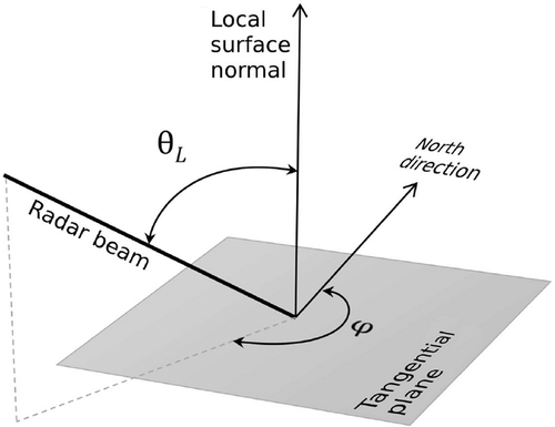
Figure 1 demonstrates that the orientation of the radar beam can be described with two angles: The local incidence angle describes the angle defined by the incident radar beam and the normal to the local surface. The azimuth angle describes the angle between the radar beam projected onto the surface and a reference direction, usually the north direction (Bartalis, Scipal, and Wagner 2006).

Figure 1. Geometric dependency of the incidence radar beam: Local incidence angle (vertical) angle and azimuth (horizontal) angle .

The radar backscatter dependency of the incidence angle is well studied (Ulaby, Moore, and Fung 1982). For most scattering targets, the backscatter decreases with increasing incidence angle and so different normalizing methods were developed (Mladenova et al. 2013). It has also been shown that over a limited incidence angle range the backscatter is approximately linear. Hence, previous studies typically applied linear models (e.g. Gauthier, Bernier, and Fortin (1998); Kennett and Li (1989); Frison and Mougin (1996); Loew, Ludwig, and Mauser (2006)), we also adopt this assumption for the Sentinel-1 backscatter model. Incidence angle normalization is done with equation (1). The backscatter , acquired at a certain local incidence angle , is normalized to a reference angle of by using the slope parameter . A reference angle of is chosen, because Sentinel-1 backscatter in IW mode is acquired within an incidence angle range of (Collecte Localisation Satellites (CLS) 2016).

(1)

In some areas the observation geometry dependency is not eliminated by simply normalizing the incidence angle. Residual effects that stem from different azimuthal viewing direction are explained by the fact that the surface of the land under observation alters the returned backscatter depending on the orientation of the tangential surface area. Bartalis, Scipal, and Wagner (2006) showed that azimuthal anisotropy is observed in scatterometer backscatter data in mountainous regions, urban areas and evenly aligned agricultural areas on a 50km scale. In addition, Stephen and Long (2002) determined azimuthal modulation over sand dunes. Since the measurement principles of scatterometer and SAR are the same, we assume that azimuthal dependency is also present in Sentinel-1 backscatter data.

2.2. Examples of azimuthal anisotropy observed

In previous scatterometer missions, azimuthal effects could be directly observed by calculating the difference between the (almost) simultaneous measurements of the fore- and aftbeam of the antenna (Bartalis, Scipal, and Wagner 2006). This technique is not possible for the Sentinel-1 SAR system. In order to investigate the effect, we separated the time series of normalized backscatter for ascending and descending passes. Areas with azimuthal anisotropy can be visualized by calculating the difference between the average of the ascending and the average of the descending of previously acquired backscatter (formula (2)). The normalized difference parameter is used to specify azimuthal modulation of the backscatter between the two overpass directions, whereby the subscript AD indicates that it is the difference between ascending and descending passes.

(2)

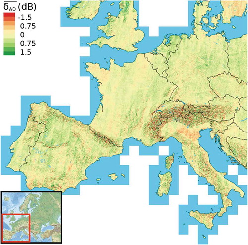
Figure 2 presents the normalized backscatter difference over Western Europe calculated from more then two years of Sentinel-1 data. The corresponding percentage frequency of the magnitude of the shift can be seen in Table 1. It can be seen that more than 50% of the surface of Europe monitored shows a shift of more than 0.25dB between the backscatter data acquired from ascending and descending orbits. The mean difference is 0.07dB, which indicates a slightly higher mean backscatter for ascending orbits. Assuming that there are no dominant topographic structures over such a large region over Europe, this would point to a systematic daily difference in backscatter due to a change in soil moisture and/or vegetation between morning and evening overpasses.

Table 1. Percentage frequency of the absolute value of the normalized backscatter difference over the area of Western Europe (Figure 2). Original dataset and after azimuth-correction of the dataset (October 2014 – December 2016).

	normalized backscatter difference
	mean	>0.25dB	>0.5dB	>0.75dB	>1dB	>1.5dB
Original	0.07dB	58.5%	30.1%	16.3%	8.7%	2.4%
Azimuth-corrected	0.0dB	6.8%	4.0%	2.8%	2.1%	1.2%

Figure 2. Normalized backscatter difference over Western Europe (October 2014 – December 2016).

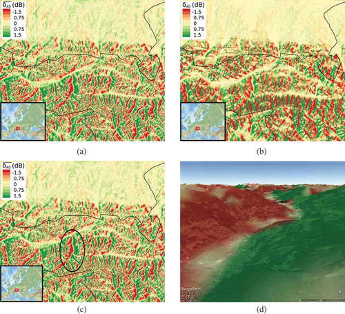
When working on this study, we also found out that the major contributor to azimuthal modulation is the orientation of the slope of the topography of the Earth’s surface. In mountainous areas like the Alps, a backscatter difference pattern can be found.

As an example, Figure 3(a) demonstrates the backscatter shift between ascending and descending passes in the Tyrolean Alps. It shows that for ascending orbits the eastern side of the valleys have a positive backscatter shift and for descending orbits this applies to the western side. Figure 3(c,d) illustrate, in more detail, the Zillertal, a valley running north-south, projected on a digital elevation model (DEM). In general, every north-south directed valley shows this pattern due to the near-polar orbit of Sentinel-1.

Figure 3. Austrian Alps: Backscatter shift due to different slope orientations: (a) Calculated from Sentinel-1 backscatter (equation (2)), and (b) modelled from SRTM-3 DEM using equation (4). (c),(d) Detail example of the Zillertal in the Tyrolean Alps.

2.3. Modelling azimuthal anisotropy using the SRTM-3 DEM

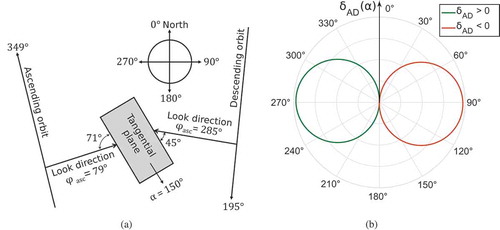
Figure 3(a) shows that the orientation of the tangential plane of a predominant slope within the radar footprint contributes most to azimuthal anisotropy. The different azimuth angles for ascending and descending overpasses observing a predominant slope is illustrated in Figure 4(a). Bartalis, Scipal, and Wagner (2006) annotated that for scatterometers with a spatial resolution of 50km, this effect is modest because on a 50km scale there is usually no preferred orientation of the slope, but for 1km Sentinel-1 data the effect is no longer negligible.

Figure 4. (a) Illustration of different azimuth angles for ascending and descending overpasses observing a predominant slope, and (b) modelled backscatter difference depending on the slope orientation . (using equation (4), with , , s = 1).

Therefore, we propose in formula (3) to model the backscatter as a function of the local incidence angle , azimuth angle and the orientation of the topography’s slope . After applying incidence angle normalization to using formula (1), the backscatter measured includes the normalized backscatter and a cosine term due to the interaction of the azimuth angle of the radar beam and the topography’s slope orientation. The cosine term is maximum when the slope faces the direction of the radar beam () and minimum if it is turned away ().

(3)

The factor s can be interpreted as a scale factor and is a function on the slope steepness.

The difference between the ascending and descending backscatter, , for each overpass direction gives a measure for the azimuthal dependency of the Sentinel-1 backscatter.

(4)

Sentinel-1 satellites orbit the Earth in a near-polar orbit with an inclination of . The azimuth angles of the ascending and descending orbits at the latitude of the Tyrolean Alps are and respectively. Therefore, the polar diagram of the backscatter shift versus the topography’s slope orientation results in a positive lobe () for a slope direction to the west and a negative lobe for a slope direction to the east () Figure 4(b). This implies that ascending orbits show a positive shift in backscatter for slopes facing west and a negative shift for those facing east. The opposite applies to descending orbits.

In equation (4), some information about the orientation of the tangential plane of the slope is needed. We determined this parameter using the SRTM-3 DEM (Jarvis et al. 2008). In addition, the scale factor s for the azimuthal modulation is derived from the SRTM-3 DEM using a Monte Carlo simulation in the interval and is set to . Figure 3(b) presents the modelled backscatter shift between ascending and descending overpasses. The mean difference of the modelled and empirical azimuthal modulation in the Tyrolean Alps is 0.14dB with a standard deviation of 0.65dB. The spatial correlation of the example presented is 0.69 and the p-value indicates that the correlation is highly significant. This result shows that the slope orientation and steepness derived from a DEM can be used to model the major contributor of azimuthal anisotropy.

2.4. Correcting azimuthal anisotropy using backscatter time series

The second option considers the azimuthal anisotropy, by using Sentinel-1 backscatter data previously acquired. This section presents an algorithm to correct the azimuthal variation when there is no information about the topography’s slope orientation. So far, more than two years of Sentinel-1 backscatter data have been available. Exactly two years of these backscatter (October 2014 – October 2016) were subsequently used to create correction parameters to avoid seasonal effects. The main idea behind this approach is to make use of the strict orbit and viewing configuration of the Sentinel-1 satellites. The orbit has a 12 days repeat cycle (6 days including Sentinel-1B) with 175 relative orbits within this repeat cycle (European Space Agency (ESA) 2013). Each measurement from a specific Sentinel-1 overpass has the same relative orbit number, and therefore, the same resulting local incidence angle. This aspect is used to group the backscatter per orbit number to get clusters of backscatter with the same local incidence angle.

The second step is setting up a statistical requirement that each cluster must fulfill. In this paper, we propose that each group of backscatter has the same average of normalized backscatter.

(5)

The reference value is the total mean of all normalized backscatter data previously acquired from all relative orbits.

(6)

If there are differences between the averages of the normalized backscatter per cluster and the reference value, the backscatter correction parameter for a particual orbit can be calculated.

(7)

By applying the parameter to the normalized backscatter , the azimuthal variation of backscatter can be corrected. The notation finally describes an incidence angle normalized and azimuthal corrected backscatter.

(8)

This algorithm implies that each cluster is normalized in relation to each other, and orbital effects – like the backscatter shift due to different azimuthal look angles – are considered. The workflow for normalizing and azimuthal correcting Sentinel-1 backscatter is shown in Figure 5(a).

Figure 5. (a) Incidence and azimuth angle normalization workflow of the Sentinel-1 backscatter data, and (b) an example of the normalization steps: (i) 2 years of Sentinel-1 backscatter observed in VV-polarisation separated by orbit number, (ii) incidence angle normalized backscatter, and (iii) normalized and azimuth-corrected backscatter.

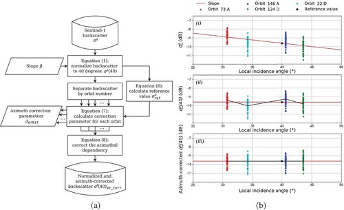
Figure 5(b) depicts the steps of the Sentinel-1 incidence and azimuth angle normalization in an area in southern Austria. This region can be characterized as a hilly region, where the azimuthal anisotropy is the result of the orientation of a predominant slope. This point on the Earth’s surface is covered by four different overpasses (two ascending and two descending), which result in four orbit clusters. Each cluster includes backscatter with the same local incidence angle. The reference is the mean of the normalized backscatter of two years of Sentinel-1 data (Figure 5(b)(i)). After normalizing the backscatter using formula (1), the incidence angle dependency is removed (Figure 5(b)(ii)). The black line connects the total mean of the backscatter per orbit and points out that each orbit shows a statistical difference to the reference total mean at . Using formula (7) the correction parameters for the azimuthal backscatter shift per orbit are calculated and the backscatter per cluster can be corrected (Figure 5(b)(iii)).

As a final result, equation (4) is used to calculate the backscatter difference of normalized and azimuthal corrected backscatter data over Western Europe. The difference between the mean of the descending and the ascending backscatter is shown in Table 1. Compared to the original data, much fewer areas reveal a shift after the azimuthal correction. Only for mountainous regions a shift can still be found. This is due to the fact that in steep terrain the linear incidence angle dependency of the backscatter is no longer valid, because this assumption is true only for a limited incidence angle range.

It must be noted that the slope – which gives information about the incidence angle dependency – is estimated from time series. After applying azimuthal correction to the backscatter data, the slope parameter can be estimated again in a second iteration step. A second remark would be that the degree of azimuthal anisotropy could have a dynamic behaviour over the year e.g. due to the vegetation cycle (Bartalis, Scipal, and Wagner 2006). This dynamic behaviour is not yet accounted for in this approach.

3. Conclusion

When using Sentinel-1 backscatter data for land studies, one should be aware of the azimuthal dependency of measurements which can cause major problems when comparing SAR images from ascending and descending passes. In this paper, two years of Sentinel-1 backscatter data over Western Europe have been analysed. It has been found out that 1km Sentinel-1 data – acquired at different azimuth angles – show differences in backscatter in areas where the land cover act as an oriented scatterer. For example, the orientation of the tangential plane of the surface in mountainous areas can alter the backscatter with more than 1.5dB between ascending and descending overpasses. The topography’s slope orientation – extracted from a SRTM-3 DEM – was subsequently used to model this azimuthal anisotropy in the Tyrolean Alps. This model is valid for lower and midlatitudes, because in these latitudes the surface is monitored from two possible azimuth angles one for ascending and one for descending orbits. For higher latitudes (e.g. polar regions), this assumption is not true any more and a different azimuth angle has to be assigned for each specific relative orbit. To enable a correction of the azimuthal anisotropy of Sentinel-1 data over all latitudes and without the need of the information about the slope orientation, a method to account for the azimuthal dependency by using previously acquired backscatter data was presented. This approach uses the strict orbit configuration of the Sentinel-1 satellites to calculate backscatter corrections for each relative orbit. Using this algorithm, areas showing backscatter difference of more than 0.25dB between ascending and descending overpasses could be reduced from 58.5% to 6.8%.

References

- Bartalis, Z., K. Scipal, and W. Wagner. 2006. “Azimuthal Anisotropy of Scatterometer Measurements over Land.” IEEE Transactions on Geoscience and Remote Sensing 44 (8): 2083–2092. doi:10.1109/TGRS.2006.872084.
- Collecte Localisation Satellites (CLS). 2016. Sentinel-1 Product Definition. European Space Agency (ESA).
- Dostálová, A., M. Doubkova, D. Sabel, B. Bauer-Marschallinger, and W. Wagner. 2014. “Seven Years of Advanced Synthetic Aperture Radar (ASAR) Global Monitoring (GM) of Surface Soil Moisture over Africa.” Remote Sensing 6 (8): 7683–7707. doi:10.3390/rs6087683.
- Early, D. S., and D. G. Long. 1997. “Azimuthal Modulation of C-Band Scatterometer σ0 over Southern Ocean Sea Ice.” IEEE Transactions on Geoscience and Remote Sensing 35 (5): 1201–1209. doi:10.1109/36.628787.
- European Space Agency (ESA). 2013. Sentinel-1 User Handbook. Retrieved from https://sentinel.esa.int/documents/247904/685163/Sentinel-1_User_Handbook
- Fraser, A. D., N. W. Young, and N. Adams. 2014. “Comparison of Microwave Backscatter Anisotropy Parameterizations of the Antarctic Ice Sheet Using Ascat.” IEEE Transactions on Geoscience and Remote Sensing 52 (3): 1583–1595. doi:10.1109/TGRS.2013.2252621.
- Frison, P. L., and E. Mougin. 1996. “Use of ERS-1 Wind Scatterometer Data over Land Surfaces.” IEEE Transactions on Geoscience and Remote Sensing 34 (2): 550–560. doi:10.1109/36.485131.
- Gauthier, Y., M. Bernier, and J.-P. Fortin. 1998. “Aspect and Incidence Angle Sensitivity in ERS-1 SAR Data.” International Journal of Remote Sensing 19 (10): 2001–2006. doi:10.1080/014311698215117.
- Jarvis, A., H. Reuter, A. Nelson, and E. Guevara (2008). Hole-Filled SRTM for the Globe Version 4, the CGIAR-CSI SRTM 90m Database, (http://srtm.csi.cgiar.org)
- Kennett, R. G., and F. K. Li. 1989. “Seasat Over-Land Scatterometer Data. I. Global Overview of the Ku-Band Backscatterer Coefficients.” IEEE Transactions on Geoscience and Remote Sensing 27 (5): 592–605. doi:10.1109/TGRS.1989.35942.
- Loew, A., R. Ludwig, and W. Mauser. 2006. “Derivation of Surface Soil Moisture from ENVISAT ASAR Wide Swath and Image Mode Data in Agricultural Areas.” IEEE Transactions on Geoscience and Remote Sensing 44 (4): 889–899. doi:10.1109/TGRS.2005.863858.
- Long, D. G., and M. R. Drinkwater. 2000. “Azimuth Variation in Microwave Scatterometer and Radiometer Data over Antarctica.” IEEE Transactions on Geoscience and Remote Sensing 38 (4): 1857–1870. doi:10.1109/36.851769.
- Mladenova, I. E., T. J. Jackson, R. Bindlish, and S. Hensley. 2013. “Incidence Angle Normalization of Radar Backscatter Data.” IEEE Transactions on Geoscience and Remote Sensing 51 (3): 1791–1804. doi:10.1109/TGRS.2012.2205264.
- Sabel, D., Z. Bartalis, W. Wagner, M. Doubkova, and J.-P. Klein. 2012. “Development of a Global Backscatter Model in Support to the Sentinel-1 Mission Design.” Remote Sensing of Environment 120: 102–112. doi:10.1016/j.rse.2011.09.028.
- Schlaffer, S., M. Chini, L. Giustarini, and P. Matgen. 2017. “Probabilistic Mapping of Flood- Induced Backscatter Changes in SAR Time Series.” International Journal of Applied Earth Observation and Geoinformation 56: 77–87. doi:10.1016/j.jag.2016.12.003.
- Stephen, H., and D. G. Long (2002). Azimuth Modulation of Backscatter from SeaWinds and ERS Scatterometers over the Saharo-Arabian Deserts. In IEEE International Geoscience and Remote Sensing Symposium, vol. 5, Toronto, ON, Canada, June 24–28, 2808–2810.
- Stephen, H., and D. G. Long (2003). Surface Statistics of the Saharan Ergs Observed in the σ0 Azimuth Modulation. In IGARSS 2003. 2003 IEEE International Geoscience and Remote Sensing Symposium. Proceedings (IEEE Cat. No.03CH37477), vol. 3, Toulouse, France, July 21–25, 1549–1551.
- Ulaby, F., R. Moore, and A. Fung. 1982. Microwave Remote Sensing: Active and Passive Volume II: Radar Remote Sensing and Surface Scattering and Emission Theory, Norwood, MA: Artech House.