Tree crown segmentation based on a tree crown density model derived from Airborne Laser Scanning

ABSTRACT

This letter describes a new algorithm for automatic tree crown delineation based on a model of tree crown density, and its validation. The tree crown density model was first used to create a correlation surface, which was then input to a standard watershed segmentation algorithm for delineation of tree crowns. The use of a model in an early step of the algorithm neatly solves the problem of scale selection. In earlier studies, correlation surfaces have been used for tree crown segmentation, involving modelling tree crowns as solid geometric shapes. The new algorithm applies a density model of tree crowns, which improves the model’s suitability for segmentation of Airborne Laser Scanning (ALS) data because laser returns are located inside tree crowns. The algorithm was validated using data acquired for 36 circular (40 m radius) field plots in southern Sweden. The algorithm detected high proportions of field-measured trees (40–97% of live trees in the 36 field plots: 85% on average). The average proportion of detected basal area (cross-sectional area of tree stems, 1.3 m above ground) was 93% (range: 84–99%). The algorithm was used with discrete return ALS point data, but the computation principle also allows delineation of tree crowns in ALS waveform data.

1. Introduction

Airborne Laser Scanning (ALS) data are highly accurate three-dimensional (3D) measurements of the ground and other objects, which are usually presented as point clouds consisting of 3D coordinates of laser return locations. Derivation of forest information from ALS data has emerged as an important application that can be used to produce accurate forest maps covering large areas, if field measurements are available as reference data (Wulder et al. 2012). It is now possible to obtain high-resolution 3D point clouds using ALS from altitudes of several thousand metres with sufficient density (>10 points/m²) to detect individual trees (Swatantran et al. 2016). This new capability can greatly facilitate sustainable management of forest resources. The tree crown segments derived from ALS data can be used for estimating attributes of trees (such as their height, stem volume, and species) and their positions (Hyyppä et al. 2008; Lindberg and Holmgren 2017).

The methods for delineating individual trees can be divided into surface model (i.e., raster) methods and 3D methods (Lindberg and Holmgren 2017). The most common surface modelling approach is to derive a Canopy Height Model (CHM) from the maximum height above the ground of all laser returns in each raster cell and identify tree tops as local maxima in the surface model. The tree crowns can then be delineated with a watershed segmentation or region growing algorithm. The use of a CHM allows application of efficient algorithms, but some information from lower vegetation layers is discarded when the surface is created. Therefore, cluster methods, which use 3D points directly (Lindberg et al. 2014), or voxel-based algorithms (Reitberger, Krzystek, and Stilla 2008) could be efficient for detecting trees in forests with multiple vegetation layers. One approach is to first delineate the trees in the top-most canopy layer from a CHM or another surface model and then use this information when analysing the entire point cloud. The point cloud can be delineated with k-means clustering, the mean shift algorithm, normalized cut, or region growing from the tree tops and downwards. Another approach is to divide the point cloud into horizontal slices of a certain vertical thickness, identify tree crowns in each slice separately, and aggregate the delineated tree crown slices to define 3D tree crowns. For an extensive review of methods for delineating individual trees, see Lindberg and Holmgren (2017).

The optimal parameter settings of tree delineation algorithms (e.g., parameters of filters) may be uncertain because they vary among forest environments. The scale selection problem, common for all tree crown delineation methods, has been solved in various ways, for example, by fitting parabolic surfaces to height data (Persson, Holmgren, and Söderman 2002). Another possibility is to use a model that can be trained using data from areas with known tree positions, for example, manually measured tree positions. New mobile sensors will probably become commonly available in the future that could provide automatically measured tree positions (Liang et al. 2014) which could be used for training of methods that detect trees from airborne sensor data. For tree crown segmentation using ALS data, we previously created a correlation surface using a geometric tree crown model (Holmgren and Lindberg 2013). The geometric tree crown model was an ellipsoid and a weight function was trained with data from areas with known tree positions. However, use of a solid geometric model is a major simplification, because laser pulses are reflected inside tree crowns.

The objectives of the study reported here were to develop and validate a new algorithm for tree crown segmentation based on novel application of a tree crown density model instead of solid shapes. For the new algorithm, ALS returns are used to represent crown density in small cells defined by height above the ground and distance from a tree’s centre. The density is calculated for all raster cells and compared with corresponding densities from density rasters derived from reference trees by calculating the correlation coefficient. For each raster cell of a correlation surface, the assigned value is the correlation coefficient obtained by comparing local 3D data with tree crown density rasters. The results validate the approach of using a tree crown density model to compute a correlation surface for automatic tree crown delineation.

2. Material and methods

2.1. Test site

The segmentation method was validated using manually measured tree positions in circular (40 m radius) field plots located at the test site Remningstorp (lat. 58°28ʹ N, long. 13°38ʹ E) in southern Sweden. The test site hosts managed hemi-boreal forest that is dominated by Norway spruce (Picea abies) but includes some Scots pine (Pinus sylvestris) and deciduous trees, mostly Birch (Betula sp.) and Oak (Quercus robur).

2.2. Airborne laser scanning data

The test site used for validation was laser-scanned with a Riegl LMS Q680i system from a helicopter during leaf-on conditions in September 2014. The laser wavelength was 1550 nm. The measurement density (i.e., density of first and single returns) was on average 83 returns/m² for ALS data within 100 m × 100 m squares that contained 40 circular 40 m radius field plots available for validation. The field of view was approximately ±30°. The flight altitude was approximately 305 m above the ground. A Digital Elevation Model (DEM) was created from the ALS data and the height of each laser return was normalized by subtracting laser return elevation values with ground elevations obtained from the DEM. The normalized ALS data were used as input to the segmentation algorithm described below. The ALS system used can produce several laser returns for each emitted pulse, and the occurrence of a return depends on the peak detection algorithm of the laser system and other energy peaks from the same emitted pulse. Therefore, only first and last returns were used in this study as input for modelling tree crown density.

2.3. Segmentation algorithm

The segmentation algorithm includes the following steps. First, creation of a tree crown density model using known tree positions. Second, creation of a correlation raster using the tree crown density model. Third, creation of a tree crown cover raster. Fourth, tree crown segmentation using both the correlation raster and a tree crown cover raster. Finally, derivation of tree crown attributes using the tree crown segmentation. These steps are described in the following sections.

2.4. Tree crown density model

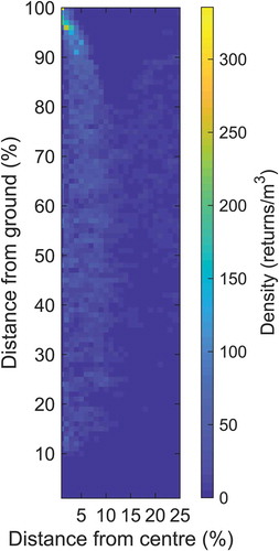
The model is a two-dimensional – height (distance above ground) x radial distance from a tree’s centre – density raster. The model can be trained with known tree positions. In this study, centre positions of trees were found in ALS data by visually inspecting 10 arbitrarily selected trees representing each of three classes (Norway spruce, Scots pine and deciduous trees). A small search distance was first used to find the maximum height in ALS data due to a peak of a tree crown. The small search distance was used because it is difficult to find the exact location of a tree peak with manual inspection. Once the peak of the tree was found it was used as the tree centre. A crown search radius from the tree centre was computed as a proportion of the tree height (i.e., the maximum height in ALS data); in this study, the radius used was a quarter of the tree height. All laser returns within the crown search radius with a height value above a threshold (set here to 2 m) were selected. The horizontal distance to the tree centre was calculated for each of the selected laser returns. Both the laser heights (i.e., distances above the ground) and horizontal distance to the tree centre were normalized by division with the maximum tree height (i.e., scale factor). In this study, a density image was created with a raster cell size of 0.01 (unitless, because the variables were normalized with the scale factor) and all raster cell values were first set to zero. A crown density model raster was created from accumulation of the number of 3D points within each raster cell (i.e., distance interval from the ground and tree centre) divided by the volume represented by this interval. The volume was derived as the area multiplied by the height of the unit represented by the interval. The area was derived as the circle with maximum radius of the raster cell interval minus the area of the circle with minimum radius of the raster cell interval, transformed back to square metres with the scale factor. The height was derived as the raster cell size in the height direction multiplied by the maximum tree height (scale factor). This accumulation procedure was repeated for all trees used to derive a tree crown density model raster. An example, of a tree crown density model raster is shown in Figure 1.

Figure 1. Example of a crown density model raster with axes according to relative distance from the centre and relative distance from the ground. The relative distances were derived as the Euclidian distance divided by the maximum distance above the ground (i.e., tree height approximation).

2.5. Correlation surface raster

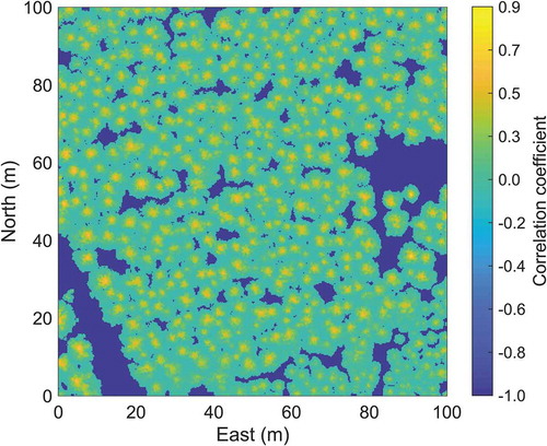
A correlation surface raster with a cell size of 0.25 m was initially created and all values were set to minus one (the lowest possible correlation coefficient). For each raster cell centre, a correlation value was calculated using the density image from the training phase. This was done by first calculating a density raster in a similar way as for the reference trees but with the potential tree centre (i.e., rotation axis) at the raster cell centre and potential tree height assigned the maximum laser height within a small search radius (in this study set to 0.2 m) from the raster cell centre. Instead of using this small search radius, the height from the corresponding raster cell value of a CHM could be used as the potential tree height, which would enhance computation efficiency. The correlation coefficient between the two rasters (i.e., the tree crown density model raster from the training phase and the crown density raster from the raster cell centre) were computed. This was repeated for all available density model rasters, in this study three (for Scots pine, Norway spruce and deciduous trees), and the highest correlation found was assigned to the raster cell of the correlation surface. An example of a correlation surface raster created using only one crown density model raster is shown in Figure 2. The correlation surface was smoothed to remove noise using a 3 × 3 filter with Gaussian weights that was applied three times to the raster.

Figure 2. Example of a correlation surface raster created from the correlation coefficients between laser data and a crown model density raster.

2.6. Tree crown cover raster

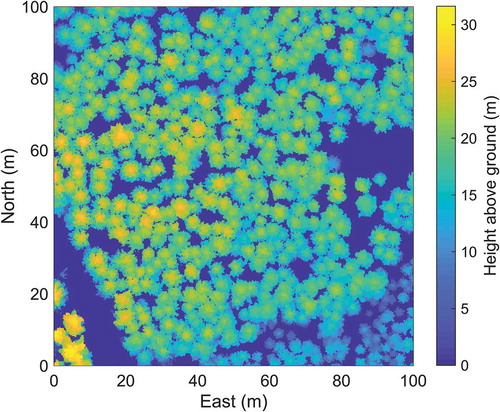
In order to create a raster showing areas with tree crowns, a CHM with a raster cell size of 0.25 m (and thus the same extent and resolution as the correlation surface raster) was created. All raster cell values were set to zero, then each raster cell that contained laser data was set to the maximum laser height (i.e., distance above ground) found in it. The tree crown cover raster was created from the CHM using a height threshold (2 m in this study, to include only trees and exclude, for instance, low vegetation or rocks). The ALS data used in this study were very dense, which enabled creation of a CHM without problems caused by raster cells with no data (Figure 3). Morphological filters were implemented to define the crown area if some raster cells were empty, so the algorithm would also be useful for sparser data (Holmgren and Lindberg 2013). The vegetation raster was binary (i.e., ‘tree crown’ or ‘no tree crown’).

Figure 3. Example of a Canopy Height Model (CHM) created by assigning a raster cell value the maximum laser-measured distance above the ground (m) within the raster cell.

2.7. Watershed segmentation

A seed was placed in each raster cell of the smoothed correlation surface that contained tree crown according to the tree crown cover raster. From each seed, a path was created by moving in the steepest direction to a neighbouring raster cell on the correlation surface. The seed locations with paths that arrived at the same local maximum formed a tree crown segment. This watershed algorithm step was the same as used in an earlier study, but in that case, a CHM was used as input (Persson, Holmgren, and Söderman 2002).

2.8. Tree crown attributes

The position of a tree was derived from the raster cell position within a segment with maximum correlation. Its height H was assigned the maximum value of raster cells of the CHM that were within the specific tree crown segment (i.e., the maximum laser height within the crown segment). The tree crown area of a segment was computed by counting the number of raster cells within the specific tree crown segment. The crown diameter was calculated using the equation for the area of a circle.

2.9. Validation

There were 40 field plots with 40 m radius at the test site with measured tree positions and stem diameters from a field inventory in 2014. Three of these plots were selected (the plot with highest proportion of Scots pine, the plot with highest proportion of deciduous trees, and the spruce-dominated plot with lowest stem density) and ALS data obtained for them were used for training the algorithm. Top positions of 10 trees in each of these plots were manually interpreted from ALS data and saved in a file with their coordinates and tree class (Scots pine, Norway spruce or deciduous trees), which was used to create three canopy density models. The three plots used for training were excluded from the validation dataset. A plot with a large amount of Hazel (Corylus avellana) was also excluded from the validation dataset because individual Hazel stems could be discerned in the ALS data, but not measured in the field inventory. Thus, its inclusion would have resulted in commission errors due to limitations of the field inventory.

The stem density in the remaining 36 field plots, which were used for validation ranged between approximately 300 and 1200 stems per hectare (Table 1). Manual field measurements of tree stem positions and stem diameters (1.3 m above ground) were acquired with a digital calliper integrated with an ultrasonic trilateration system (DP POSTEX, Haglöf Sweden AB). The ultrasonic trilateration system measures tree positions relative to a plot centre, but only has sufficient accuracy for short distances, up to approximately 15 m from the plot centre. Therefore, a grid of 4 × 4 sub-plots was used to cover each 40 m radius plot. Terrestrial Laser Scanning (TLS) data from a ground-based laser scanner placed on 4 × 4 scan stations were used for co-registration of manually measured coordinates of trees in different sub-plots to be included in a common coordinate system. First, individual point clouds from scan stations were merged with co-registration using spheres placed on adjacent scan stations. Trees were then detected and stem diameters were estimated from TLS data using a previously developed algorithm (Olofsson and Holmgren 2016). The manual field measurements of tree positions and stem diameters from sub-plots were then automatically linked to the spatial pattern of tree positions from TLS measurements in the common coordinate system using a previously developed tree-matching algorithm (Olofsson, Lindberg, and Holmgren 2008). The same tree-matching algorithm was also used for automatically linking trees found in ALS data using the new segmentation algorithm with the field-measured trees used for validation. Trees with a stem diameter ≥4 cm at 1.3 m above ground were field-measured and used for the validation. The omission error was defined as a proportion (%) of field-measured trees that were not linked to a detected tree and the commission error was defined as a proportion (%) of detected trees that were not linked to a field-measured tree. The proportion detected trees (%) was defined as proportion of field-measured trees that were linked to a tree found in ALS data.

Table 1. Forest attributes and tree detection results in the 36 field plots used for validation, presented as summary values of field plots. The basal area is the cross-sectional area of the tree stem at 1.3 m above ground, H² is the square of the tree height, STD is standard deviation, and Q are quantiles.

Variable	Mean	STD	Q25	Q50	Q75	Min	Max
Stem density of live field measured trees (ha^−1)	626	216	447	610	744	304	1182
Mean diameter (mm) at breast height (1.3 m above ground) of live field measured trees	249	57	199	245	294	157	385
Proportion of live field-measured trees linked to a detected tree (%)	85	12	82	87	93	40	97
Sum of basal area of linked live field-measured trees divided by sum of basal area of all live field-measured trees (%)	93	5	91	94	97	84	99
Proportion of detected trees not linked to a field-measured tree (%)	18	13	9	15	22	3	60
Sum of H^2 of unlinked detected trees divided by sum of H^2 of all detected trees (%)	13	9	6	10	19	1	47

3. Results

High proportions of field-measured trees in the plots (85% of live trees on average, range 40–97%, and 82% of field-measured trees including standing dead trees) could be automatically linked to trees found in the ALS data. Detected and linked field-measured trees accounted for even higher proportions (93%, on average) of the basal area (cross-section area of tree stems, 1.3 m above ground), because the detection rate was higher for tall trees than for smaller trees (Table 1). Comparison of stem diameter distributions of detected and all field-measured trees confirmed the correlation between trees’ detectability and size (Figure 4). The commission errors were on average 18% for the plots, but varied strongly among them, ranging between 3% and 60% because of extreme values for some plots, as confirmed by the quantiles (Table 1). The commission errors were more common for small trees than for tall trees, according to the ratio of sums of squares of heights of trees that were detected but not linked to a manually measured tree, and heights of all detected trees (Table 1).

Figure 4. Stem diameters at 1.3 m above ground of live field-measured trees in the 36 field plots used for validation (All field trees) and stem diameters of the subset of trees detected using the algorithm and linked to field-measured trees (Detected field trees).

4. Discussion

The new segmentation algorithm efficiently delineated tree crowns despite a simple implementation. It is suitable for analysis of large datasets because of the simple implementation that includes only a few calculation steps. A dataset with known tree positions was needed for the training phase, but only 30 trees were used in this study (10 from each of three tree classes). A precursor of the algorithm, with a solid geometric model, was validated at the same test site in a benchmarking study together with other algorithms. The precursor was tested in Sweden, Norway, Germany and Brazil (Vauhkonen et al. 2011). Its omission error was reportedly 31% (lower than rates obtained using five other algorithms tested in the cited study) at the Swedish test site, also used in this study, in which 17 field plots were used for validation. In this study, use of a density model instead of a solid geometric model resulted in an average omission error of 15% for live trees (85% of the field trees were detected) and the stem density was on average slightly higher in 36 field plots than in the 17 field plots used in the earlier benchmarking study. In this study, data for individual trees were aggregated to derive tree crown model rasters for three classes of trees (Scots pine, Norway spruce, and deciduous trees). However, more tree crown model rasters could be derived for trees in different categories, for example, tree species with different crown shapes or densities. Inclusion of a model trained with empirical data in the new algorithm enables use of only a few parameters. Some of the thresholds used are soft because the results are not sensitive to a precise value, e.g., the expected maximum ratio between crown radius and tree height used as the search distance from a tree centre. Others can be set by applying fundamental physical knowledge (e.g., the height threshold). A limitation in forests with irregular tree crown shapes is an assumption that tree crowns have radial symmetry.

The segmentation method had high accuracy according to the validation tests, which may have been partly due to use of high-resolution ALS data. In future studies, the algorithm should also be validated using ALS data with lower resolution because the canopy density raster would then be sparser. However, the step of the algorithm in which correlation coefficients are calculated allows applications where the ALS data resolution varies because of the inherent normalisation with mean values of the equation used to calculate the correlation coefficient. It is possible that more tree crowns will be needed for the training phase if only sparse ALS data are available, to accumulate sufficient laser returns to derive a tree crown density model raster with the same accuracy.

The presented algorithm could also be suitable for processing waveform data (i.e., ALS data with a histogram of returned power along a vector derived from the beam direction) or single photon laser data where each point corresponds to a photon. The 3D point clouds derived from ALS are only positions of the peaks in the waveform of returned power, which is usually discarded at an early stage of the data processing. Instead of the 3D point data used in this study, amplitudes of the waveforms could be inserted into the crown density model raster. It is also possible to use waveform attribute data associated with each point of the 3D point cloud to build the crown density models. Different ways to create tree crown density models should be explored in future studies.

Acknowledgments

We are grateful for the support from Kenneth Olofsson who developed the tree-matching algorithm used for validation. We would like to thank Tommy Andersson and Axel Bergsten for collection of the field inventory data.

Additional information

Funding

Brattåsstiftelsen för Skogsvetenskaplig Forskning (The Brattås Foundation for Forest Science Research); Carl Tryggers Stiftelse för Vetenskaplig Forskning (Carl Trygger's Foundation for Scientific Research); Hildur och Sven Wingquists Stiftelse för Skogsvetenskaplig Forskning (Hildur and Sven Wingquist's Foundation for Forest Science Research).

References

- Holmgren, J., and E. Lindberg. 2013. “Tree Crown Segmentation Based on a Geometric Tree Crown Model for Prediction of Forest Variables.” Canadian Journal of Remote Sensing 39: S86–S98. doi:10.5589/m13-025.
- Hyyppä, J., H. Hyyppä, D. Leckie, F. Gougeon, X. Yu, and M. Maltamo. 2008. “Review of Methods of Small-Footprint Airborne Laser Scanning for Extracting Forest Inventory Data in Boreal Forests.” International Journal of Remote Sensing 29: 1339–1366. doi:10.1080/01431160701736489.
- Liang, X., A. Kukko, H. Kaartinen, J. Hyyppä, X. Yu, A. Jaakkola, and Y. Wang. 2014. “Possibilities of a Personal Laser Scanning System for Forest Mapping and Ecosystem Services.” Sensors 14 (1): 1228–1248. doi:10.3390/s140101228.
- Lindberg, E., L. Eysn, M. Hollaus, J. Holmgren, and N. Pfeifer. 2014. “Delineation of Tree Crowns and Tree Species Classification from Full-Waveform Airborne Laser Scanning Data Using 3-D Ellipsoidal Clustering.” IEEE Journal of Selected Topics in Applied Earth Observations and Remote Sensing 7 (7): 3174–3181. doi:10.1109/jstars.2014.2331276.
- Lindberg, E., and J. Holmgren. 2017. “Individual Tree Crown Methods for 3D Data from Remote Sensing.” Current Forestry Reports 3 (1): 19–31. doi:10.1007/s40725-017-0051-6.
- Olofsson, K., and J. Holmgren. 2016. “Single Tree Stem Profile Detection Using Terrestrial Laser Scanner Data, Flatness Saliency Features and Curvature Properties.” Forests 7 (9): 207. doi:http://dx.doi.org/10.3390/f7090207.
- Olofsson, K., E. Lindberg, and J. Holmgren. 2008. “A Method for Linking Field-Surveyed and Aerial-Detected Single Trees Using Cross Correlation of Position Images and the Optimization of Weighted Tree List Graphs.” In Edited by R. Hill, J. Rosette, and J. Suarez, Proceedings of SilviLaser 2008, 8th international conference on LiDAR applications in forest assessment and inventory, Edinburgh, UK: Heriot-Watt University, September 17–19.
- Persson, Å., J. Holmgren, and U. Söderman. 2002. “Detecting and Measuring Individual Trees Using an Airborne Laser Scanner.” Photogrammetric Engineering and Remote Sensing 68: 925–932.
- Reitberger, J., P. Krzystek, and U. Stilla. 2008. “Analysis of Full Waveform LIDAR Data for the Classification of Deciduous and Coniferous Trees.” International Journal of Remote Sensing 29: 1407–1431. doi:10.1080/01431160701736448.
- Swatantran, A., H. Tang, T. Barrett, P. DeCola, and R. Dubayah. 2016. “Rapid, High-Resolution Forest Structure and Terrain Mapping over Large Areas Using Single Photon Lidar.” Scientific Reports 6. doi:10.1038/srep28277.
- Vauhkonen, J., L. Ene, S. Gupta, J. Heinzel, J. Holmgren, J. Pitkanen, S. Solberg, et al. 2011. “Comparative Testing of Single-Tree Detection Algorithms under Different Types of Forest.” Forestry 85: 27–40. doi:10.1093/forestry/cpr051.
- Wulder, M. A., J. C. White, R. F. Nelson, E. Næsset, H. O. Ørka, N. C. Coops, T. Hilker, C. W. Bater, and T. Gobakken. 2012. “Lidar Sampling for Large-Area Forest Characterization: A Review.” Remote Sensing of Environment 121: 196–209. doi:10.1016/j.rse.2012.02.001.