Exploring the link between supply and demand of cultural ecosystem services – towards an integrated vulnerability assessment

Abstract

Vulnerability studies need to consider changes in the ecological and the social system as well as their interactions. Yet, the link between ecosystem services and the wellbeing of different social groups represents a deficit in research. The presented case study attempts to create a deepened understanding of the social–ecological system as a basis for vulnerability assessment. For this purpose, participatory mapping of cultural ecosystem services (CES) and perceived vulnerability in the urban region of Rostock (Germany) were conducted. A comprehensive approach was developed including the spatial distribution of CES in the urban region, the interrelations between the supply and demand of CES (considering different social factors and the spatial link), as well as an exemplary vulnerability assessment. The case study showed that an application of the participatory mapping approach is valuable in a wide urban region. The evaluation of the link between population wellbeing and CES suggested no differences according to social factors. Concerning the spatial link, different critical distances for individual CES were found. An integrated map of supply and demand was developed showing the supply of districts with CES area, number, and diversity. The final exemplary vulnerability assessment visualized potential changes in CES supply areas and affected districts in the urban region.

Keywords:

• cultural ecosystem services
• participatory assessment
• perceived vulnerability
• social–ecological systems
• supply–demand interaction
• urban region

1. Introduction

In urban regions, the social and the ecological systems interact in a confined space resulting in multifaceted dynamics, where landscape changes are driven by strongly interrelated factors like land use change, population development, and cultural transformations. That sets up the basis upon which climate change will act, causing or exacerbating problems (Gasper et al. 2011; Hunt & Watkiss 2011). On the Baltic coast, sea-level rise and the risk of flooding and other extreme events are expected to increase (IPCC 2012). Compared with the rest of the world, impacts are moderate, but it is clear that climate change will have a considerable effect on the quality of life in Europe (EEA 2009). The vulnerability concept deals with the complex dynamics of the coupled human–environment system (Turner et al. 2003) and the assessment can be approached in very different ways (Preston et al. 2011). The potential of combining of the conceptual frameworks of vulnerability and ecosystem services has been shown by several studies (Maxim & Spangenberg 2003; De Chazal et al. 2008; Rounsevell et al. 2010). Rounsevell et al. (2010) proposed the ‘Framework for Ecosystem Service Provision’ explicitly addressing the fact that state variables need to involve both, social attributes of people benefitting and ecological attributes related to the provision of services. As such, in the context of climate-change research it needs to be acknowledged that climate change acts upon social and ecological aspects simultaneously. On the one hand, ecosystems could be influenced and thus the ecosystem service supply capacity. On the other hand, the population wellbeing could be affected and thus the ecosystem service demand (Beichler et al. 2012). Consequently, a methodological approach needs to consider the potential change of the demand of different social groups, the supply of different ecosystems, and supply–demand interactions (Beichler et al. 2012). However, there is a research deficit regarding the link between ecosystem services and the wellbeing of different social groups (Daily et al. 2009; Granek et al. 2010).

The local supply of ecosystem services can generate benefits at other scales (De Groot et al. 2010), which is of special interest for urban regions in terms of rural–urban gradients (Kroll et al. 2012; Larondelle & Haase 2013; Radford & James 2013). Hence, it is important to assess and compare ecosystem service supply or service providing area and demand or benefitting area as emphasized by several recent case studies (Burkhard et al. 2012; Syrbe & Walz 2012; Schulp et al. 2014; Stürck et al. 2014). First attempts to characterize the spatial interrelations between supply and demand have been made assessing structures of the social network in the context of ecosystem management (Ernstson 2013). However, the specific link between supply and demand is not well understood, especially when it comes to the influence of social factors. Against this background, the objective of this paper is to develop an assessment method to understand the vulnerability of social–ecological systems. Thereby the case study is aimed at identifying the link between ecosystem service supply and demand as well as ecosystem services and wellbeing integrating several social factors into the assessment.

While the body of literature on ecosystem service assessments is rapidly growing (Martínez-Harms & Balvanera 2012), the assessment of cultural ecosystem services (CES) lags behind as they are intangible, subjective, and difficult to evaluate (Chan et al. 2012; Daniel et al. 2012). However, due to this dependence on social constructs, CES are particularly suitable to study the link between population wellbeing and ecosystem services, considering the directly perceivable benefits derived from CES such as recreation. In addition, a case study on CES is particularly suitable when combining vulnerability and CES assessment, as for both there is a call for stakeholder participation. By taking a participatory approach, one could on the one hand account for local vulnerability characteristics (Hunt & Watkiss 2011; Hutton et al. 2011). On the other hand, it is possible to bring local experiences of stakeholders into a spatial context (Brown et al. 2012; Fagerholm et al. 2012) and indicate the importance of ecosystem services in terms of wellbeing (Maynard et al. 2011).

Against this background, the case study attempts to create a deepened understanding of the social–ecological system as a basis for vulnerability assessment. To achieve this objective a case study on CES in an urban region on the Baltic Sea coast was conducted. A participatory mapping approach was adopted acquiring empirical data on perceived vulnerability and CES in the urban region of Rostock (Germany). A comprehensive methodological approach was developed to characterize the CES supply and the demand answering the following questions: How are CES distributed in the urban region? Are individual CES valued differently according to social factors? Do the spatial interrelations of supply and demand differ between individual CES or according to social factors? Through the characterization of the social–ecological system an integrated CES supply–demand map is revealed that serves as a basis for an exemplary vulnerability assessment.

2. Methods

This section first introduces the case study area and the method by which the empirical data were acquired in a participatory way. The following description outlines the spatial analysis and statistics conducted, including several consecutive methods that have been applied.

2.1. Case study area and database

The city of Rostock is situated in the north of Germany and belongs to the federated state of Mecklenburg-West Pomerania. The city itself comprises an area of 181 km² with a population of ca. 199,380 (in 2009). The urban region (Figure 1a) under consideration additionally includes all adjacent municipalities, thus accounting for ca. 553 km² and an overall population of 245,981 (in 2009). The brackish water estuary of the River Warnow (called Unterwarnow) divides the city into a western part where most residential development is found and an eastern part that is influenced by the harbor and industrial sites. The city center is at the transition of the River Warnow to its widened estuary. In the north, the urban region is bounded by the Baltic Sea. The huge forested area (ca. 60 km²) in the northeast is called Rostocker Heide.

Figure 1. The urban region of Rostock. (a) Digital topographical map (DTK). (b) The population per living area alongside the administrative boundaries of the individual districts belonging to the city and the overall urban region.

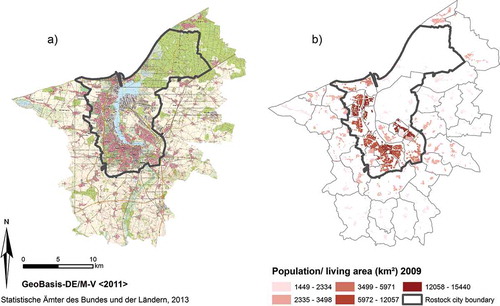
The administrative borders (Figure 1b) include 21 city districts and 24 municipalities, for which statistical data are available (Statistische Ämter des Bundes und der Länder, accessed 2013). Based on the information in the digital topographical map (DTK 25, ©GeoBasis-DE/M-V(2011)), the population data of the overall district/municipality was transferred to the shape of the available living area in the specific districts/municipalities.

2.2. Participatory mapping

The participatory mapping was administered in six group sessions and lasted 1–1.5 h. Organizations and institutions with different backgrounds were contacted to get a person on site to organize a room and invite other participants to form a group of 4–7 people. The 36 participants represented local planning institutions, economic organizations, an environmental and a social NGO, a civil protection department, and a science department. During the process, participants were asked to map only places they had visited before. The group environment positively influenced the participatory process (Hagemeier-Klose et al. 2014). The results from the different groups were compared, revealing no significant differences. Thus, the interaction within the groups and the background of participants were ruled out as an influencing factor for this case study. All participants were therefore treated individually for the analysis. Moreover, every participant filled in an extensive survey. Adapted from Fagerholm et al. (2012) and Brown et al. (2012), the survey questions included general data (gender, age, etc.), the participants’ living district/municipality, and a ranking (1–5) with regard to local knowledge, leisure time spent outdoors, and ecological knowledge (see Figure 3 for a full list of social factors assessed).

The group sessions included a survey, the mapping, and the ranking with regard to the importance of every single service. Hence, to assure a reasonable timeframe the case study was restricted to CES. The individual CES were selected based on literature in an attempt to assure completeness, comparability, and applicability. On the one hand, different classification systems (De Groot et al. 2002; MEA 2005; Burkhard, Kroll, et al. 2010; Hermann et al. 2011; Crossman et al. 2013) were considered to come up with a complete list of potential CES to be assessed. On the other hand, different participatory approaches (Raymond et al. 2009; Bryan et al. 2010; Niemelä et al. 2010; Sherrouse et al. 2011; Brown et al. 2012; Brown & Reed 2012; Fagerholm et al. 2012; Koschke et al. 2012) were compared reflecting the list of CES. Based on the results obtained by previous studies and their method of discussion, the list of CES was adjusted mainly by merging some of the subclasses. Thus, the final set of six CES included aesthetics and inspiration (aest), spiritual and religious (spirit), cultural heritage and identity (cult), recreation (recr), knowledge and education (edu), and natural heritage and intrinsic value of biodiversity (nat).

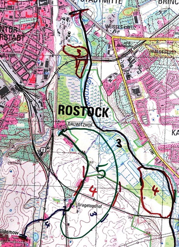
The participatory mapping method was adopted after Fagerholm et al. (2012) and Fagerholm and Käyhkö (2009) using printed topographical maps (ca. 2 m × 2 m) (Figure 1a), one for each of the CES. Additional material for baseline reference (such as a roadmap) was provided but was never used. The individual CES were translated into easily accessible questions (adopted after Plieninger et al. 2013), for example, ‘Which places do you value due to the aesthetics and inspiration they convey?’ An exemplary result of the mapping procedure is shown in Figure 2. The participants were equipped with individually colored pens for the mapping to assure that the areas mapped can subsequently be assigned to the individual survey data. The participants were free to delineated areas, linear structures or positions, but in the introduction of the method, the importance of the spatial context of the entries was emphasized. As such, participants were asked to use lines only in cases where the service was related to a linear structure, for example, along a green promenade. If the service was related to, for example, the broad view along a hiking path, then the overall area was delineated not only the path itself. Furthermore, for each individual entry on the map the participants allocated quality values from 0 (no quality) to 5 (very high quality) (see Figure 2).

Figure 2. Example of the raw data received from the participatory mapping exercise.

After finishing a map the participants were asked to fill in a table ranking the importance of the service for their personal wellbeing: 1 (not important) to 5 (very important) (Koschke et al. 2012). This was complemented by the ranking of satisfaction with the service supply: 1 (not satisfied) to 5 (very satisfied) in the urban region of Rostock. Wellbeing is a concept with different meanings, potential definitions, and facets. According to the differentiation of Summers et al. (2012), these are (1) basic human needs (provisioning services, natural space, education), (2) economic wellbeing, (3) environmental needs (regulating services), and (4) subjective wellbeing or happiness. The latter was emphasized in this assessment while acknowledging that it also relates to various interdependent factors like education, health, natural environment, culture, and recreation. Considering this context, satisfaction would actually be a subcategory of subjective wellbeing. However, the different rankings according to wellbeing and satisfaction intend to provide a measure of the benefits that could (what is important) and should (how much) be provided.

Following the mapping of all CES, the participants were asked to map out areas they would avoid during or after climatic extreme events of a heat wave, extreme precipitation, or a drought. This participatory vulnerability assessment considered extreme events that occurred in the region during the last years, thus events that could directly be perceived by participants (Hagemeier-Klose et al. 2014). The mapping procedure followed the same rules as already described. However, instead of quality ranks the participants indicated the type of extreme event for the individual entry.

The maps were digitized (photographed and geo-referenced) in ArcGIS 10 while retaining the participants’ ID to allow the areas to be associated with the survey answers and rankings. In order to retain the structure but analyze the spatial context and extent, lines and points were treated as areas, applying a 20 m buffer to the raw data.

2.3. Spatial analysis and statistics

The overall research roadmap is depicted in Figure 3. The data derived from the participatory mapping were prepared to characterize the supply and the demand side by means of the spatial distribution of CES and the grouping of the social factors, respectively. In the first step, the categorical link between supply and demand of CES was investigated, to answer the question whether the individual CES are valued differently according to social factors. In the second step, the spatial link between the supply and demand of CES was analyzed, to answer the question whether the distance to CES areas differ between the individual CES or according to social factors. The results of the previous steps serve as input for an integrated map of supply and demand. Subsequently, the supply–demand map and the data on perceived vulnerability were combined to indicate changes in the CES.

Figure 3. Research roadmap.

2.3.1. Spatial distribution of CES

The raw data on the CES distribution were characterized in terms of number and type of entries, as well as the spatial extents for the individual services, in order to reflect upon the participatory method used. In the second step, the overlap within CES classes was corrected, clustering the data based on the six individual CES. The raw data and the clustered data were compared to verify that multiple participants delineated the CES areas. The resulting maps served as a basis for the characterization of the urban region in terms of CES supply.

2.3.2. Categorical link – social factors and CES

The ranking data on wellbeing and satisfaction were compared between the individual CES. In order to establish the link between wellbeing, social factors, and the different CES, the results were evaluated based on the 16 social factors derived through the survey information (see Figure 3 for a full list of factors). The information on social factors was aggregated to 2–3 groups of at least 8 participants to ensure statistical testability. To exemplify, the survey contained information on the number of children, which was reduced to ‘children: yes or no.’ Moreover, due to the limited number of participants, it was not possible to combine social factors to form social groups. The final comparisons of social factors and the different CES were displayed using grouped box plots. The statistical analysis was performed in SPSS 20 using the Kruskal–Wallis test (confidence interval 99, significance level 0.01).

2.3.3. Spatial link – distance to home

The survey information on the participants’ living districts/municipalities was transferred to the map with the administrative areas of the urban region (cf. Figure 1b). The distance to home (DTH) was calculated assessing Euclidian distances between home district of the participant and the individual CES entries (Fagerholm & Käyhkö 2009). The spatial link between supply and demand of CES is the central measure, therefore the DTH was reflected carefully considering different potential dependencies (cf. doted arrows in Figure 3). The DTHs of the individual CES were compared with regard to minimum and maximum, mean and median distances. The correlation between DTH and the quality value of the CES areas was considered as well. Moreover, the DTHs were reflected based on the ranking of the participants in terms of wellbeing and satisfaction. To identify potential differences for social factors, the DTHs were then reflected, also taking the other survey information on social factors (age, car ownership, etc.) into account.

2.3.4. Integrated supply–demand

In order to combine the supply information on the CES with the demand information, a neighborhood analysis was conducted. The input maps (cf. hexagons in Figure 3) and distances for this analysis were based on the previous results. As such, the demand side results of the case study participants were transferred to the overall population, hereby differences identified according to social factors (categorical) should be reflected in the population distribution. However, since no differences were identified for this case study, the population data were not differentiated according to social factors. The same is true for the distances, here no differences were found according to social factors, and as such, the same distances for the overall population were applied. For the supply side, differences for the individual CES were found in terms of distance. Thus, the different median DTHs for the individual CES served as critical distances for this analysis. The method allows for two different applications taking either the supply side (CES areas) or demand side (population data) as output map. In this case study, all service areas within the critical distance were counted as supply to the individual district/municipality, with the population shape as output map. As the overall purpose is to show application of the developed method, for the purpose of simplicity, the calculation of the supply per person was refrained. Based on the neighborhood analysis, the results for the individual CES were accumulated in terms of CES supply area and number. Moreover, taking all CES together the service diversity was revealed, reflecting the number of different CES supplied. The resulting map was used to identify hot-spots and cold-spots within the case study area, and to indicate districts with undersupply.

2.3.5. Exemplary vulnerability assessment

There are various different approaches to assess vulnerability (Preston et al. 2011). Hereby, the exposure map usually is derived through modeling of climate variables representing future changes (e.g., in temperature). In the current case study, the exposure variable is not future directed. Being aware of the limitations, it is referred to as exemplary assessment aimed at illustrating the potential use of the integrated supply–demand map in vulnerability assessments. The extreme events considered in the mapping of perceived vulnerability occur already today. Although, the perceived vulnerability does not necessarily correspond to the actual exposure, in the case of CES the service benefit is lost if the places are not visited. Thus, using the areas of perceived vulnerability as exposure variable in the exemplary assessment, the results indicate today’s vulnerability to drought, heat wave, and extreme precipitation.

The data on perceived vulnerability were treated in the same way as the CES data (cf. Section 2.3.1). The subsequent, spatial overlay of the maps of perceived vulnerability and the CES supply indicated the potential loss of CES supply areas. To illustrate the changes for individual districts/municipalities (demand side), areas of perceived vulnerability excluded from the neighborhood analysis (cf. Section 2.3.4) and subsequent calculations were repeated using the same DTH as before. For the comparison of the results, the same color scheme and range as in the previous supply–demand map was applied. The differences between the integrated supply–demand maps indicate the vulnerability regarding a decreased supply in terms of CES area, number, and diversity.

3. Results

This section is divided into five parts. The first deals with the spatial characterization of the urban region of Rostock, illustrating the results of the participatory mapping exercise and local characteristics derived thereof. Afterward the results of the analysis of the categorical and the spatial link between CES supply and demand are shown. Lastly, the integrated CES supply–demand map and the vulnerability assessment are presented.

3.1. Spatial characterization of the urban region – supply side

A substantial amount of data could be revealed through the participatory mapping approach, which is attributable to the positive impact of the group dynamics on the motivation, as reported in Hagemeier-Klose et al. (2014). Altogether participants identified 674 areas, 157 linear structures, and 123 positions, the descriptive spatial statistics are shown in Figure 4. Most entries were related to aest (229) and recr (214), and the least entries were made for edu (124) and spirit (67), as reflected by the total area of the raw data (Figure 4). The service area after the correction of overlaps within themes is considerably reduced compared with the raw data, illustrating that entries were frequently repeated in the same location, and therewith verified (Hagemeier-Klose et al. 2014). The class of spirit is an exception here, as only very few entries were verified, indicating that places with spiritual and religious values are individually perceived. This was confirmed by participants’ references to personal and intimate experiences during the mapping process. Consequently, spirit was excluded from subsequent analysis, because the entries represented only the experience or perception of one person. The processing of the raw data resulted in the following number of areas: 29 aest, 21 cult, 26 recr, 45 edu, and 26 nat, which represent the supply of CES in the urban region of Rostock as illustrated in Figure 5a–e.

Figure 4. Areal statistics of the different cultural ecosystem services (spiritual and religious (spirit), knowledge and education (edu), cultural heritage and identity (cult), aesthetics and inspiration (aest), recreation (recr), natural heritage and intrinsic value of biodiversity (nat)) including the total area of the raw data from the participatory exercise, the corrected service area after dissolving the raw data, and the remaining service area after erasing the areas of perceived climate change impacts (CC service area).

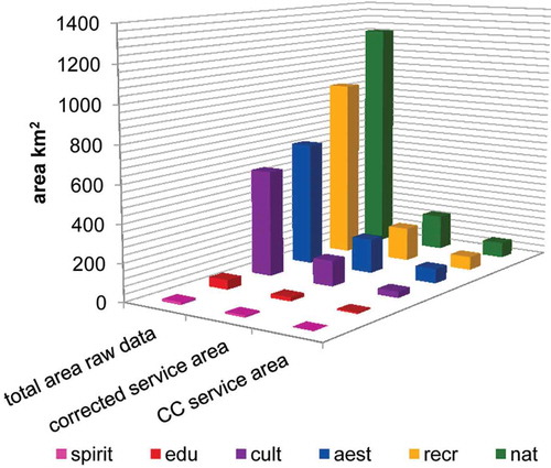
Figure 5. Maps of the corrected service area of the individual cultural ecosystem services: (a) aesthetics and inspiration (aest), (b) cultural heritage and identity (cult), (c) knowledge and education (edu), (d) recreation (recr), and (e) natural heritage and intrinsic value of biodiversity (nat). The higher the quality ranks for the CES areas, the darker the color (see individual legends). (f) Map of the perceived vulnerability to drought (D), heat (H), and extreme precipitation (S). The population per living area is depicted in the background.

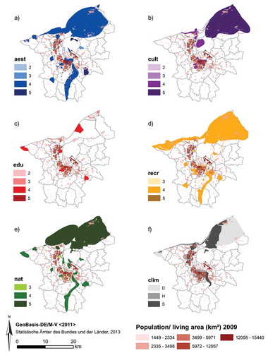
The maps of the individual CES reveal local characteristics of the case study area. General hot-spots for all CES (cf. Figure 5) can be identified, especially on the Baltic Sea coast. First, in the northeast the large areas refer to the site called Rostocker Heide. Second, a part of the coastline (west of the river) divides into two parts, east is a tourist hot-spot area called Warnemünde with a white sandy beach and a promenade; in the western part, the coast is steeper and located in the nature reserve areas called Stolteraa, where there is a hiking trail. Third, the many small areas in the middle of the map refer to the city center. The results indicate that areas valued for aest, recr, and nat often coexist, for example, the riverside in the south and the nature reserve in the far west. In terms of cult, the importance of the harbor (mid-north) was highlighted.

3.2. Categorical link – social factors and CES

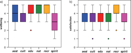
In general, most of the participants ranked importance of CES for wellbeing as well as satisfaction with supply in the urban region as high. The importance for wellbeing (Figure 6a) was significantly (p < 0.0001) higher for nat and recr, and lower for spirit. The satisfaction with supply (Figure 6b) was significantly (p < 0.001) higher for recr. Except for spirit, importance for wellbeing was given a higher ranking than satisfaction with supply. Interestingly, neither the total area of the services delineated (cf. Figure 4) nor the number of the areas delineated did directly relate to importance for wellbeing or overall satisfaction with the supply in the urban region. For example, aest with 229 entries and edu with 124 displayed the same mean for satisfaction (3.59; 3.66) and wellbeing (3.97; 4.03).

Figure 6. The boxplots illustrate the ranking according to the importance of the individual cultural ecosystem service (aesthetics and inspiration (aest), cultural heritage and identity (cult), knowledge and education (edu), natural heritage and intrinsic value of biodiversity (nat), recreation (recr), spiritual and religious (spirit)) for wellbeing (a) and (b) satisfaction with supply in the urban region.

The ranking of the importance for wellbeing and of the satisfaction with supply in the urban region were compared for the individual CES with regard to each of the 16 different social factors. Although, the survey data partially contained more detailed information, to ensure statistical testability (n ≥ 8) the social factors were grouped as follows: residence (city, hinterland), duration of residence (<10, 10–30, >30 years), gender, age (<35, 35–50, >50), children (yes, no), marital status (married, other), house type (detached, block, multi/terraced/duplex), garden (yes, no), residential property (yes, no), car ownership (yes, no), level of education (A level – German Abitur, secondary – German mittlere Reife), employment (full-time, not full-time), income in Euro per month (more than 3000, less than 3000). Furthermore, the participants’ ranking data (1, very poor–5, very good) were aggregated (to assure n ≥ 8) for local knowledge (2 and 3; 4 and 5), ecological knowledge (2 and 3; 4; 5), and leisure time spent outdoors (3 and 4; 5). The comparisons of the social factor groups are depicted by means of grouped boxplots for the individual CES in terms of wellbeing (1, not important–5, very important) in Figure 9 (see Supplemental data) and for satisfaction (1, not satisfied–5, fully satisfied) in Figure 10 (see Supplemental data).

In general, nearly no differences according to social factors for either wellbeing or satisfaction were found. The results show one significant difference (p < 0.01) for wellbeing (see Supplemental data) indicating that people with an income of more than 3000 € netto per month ranked edu to be less important (Figure 9p). Trends (p < 0.05) indicated that for people living in the city cult was more important for their wellbeing (Figure 9a) and aest was less important to married people (Figure 9f). In terms of satisfaction (see Supplemental data) also one significant difference (p < 0.01) was found indicating that the older the people, the higher was the ranking for satisfaction with supply of nat (Figure 10d). A similar trend (p < 0.05) was found for satisfaction with nat according to the duration of residence (Figure 10b). Moreover, a trend suggested that women were more satisfied with the supply of edu and recr (Figure 10c). However, the differences revealed showed no general tendency, but the trends detected could be of interest for future studies. The most interesting finding was where no differences were found. In the case study, no difference between people with children or without children, and according to house type, access to a garden, car ownership, employment, level of education, local knowledge, ecological knowledge, etc. (cf. Figure 9 see Supplemental data and Figure 10 see Supplemental data) could be observed.

3.3. Spatial link – distance to home

The DTHs for the individual CES are depicted in Figure 7. The boxplot shows that for all CES the DTHs calculated were subject to large-scale fluctuations. The DTHs ranged from a minimum value of 0 to a maximum value of 21 km for aest, for cult 0–20 km, edu 0–18 km, nat 0–21 km, and recr 0–19 km. The mean values for the CES differed: aest 4.9 km, cult 3.8 km, edu 4.3 km, nat 6.7 km, and recr 5.1 km. The standard deviation was, however, particularly high, for example, 4.8 for nat. The results obtained can be explained by the design of the study. Here, several factors need to be considered when interpreting the statistics. On the one hand, the DTHs for all CES included many zero and very low values, meaning that these areas are located within or very close to the home district, thus places that participants were most familiar with. On the other hand, maximum values indicated the distance at which the different service areas were still recognized. This absolute maximum distance was around 20 km for all CES, but differed between the individual participants. The mean of all individual maximum values shows a more distinct picture: aest 11 km, cult 9 km, edu 9 km, nat 13 km, and recr 11 km. Most of these high-distance CES areas were ranked as being of high (4) or very high (5) quality. Nevertheless, there was no linear correlation between DTH and quality ranks. Furthermore, it was found that there is no indication that the DTH was related to any of the 16 different social factors. For example, there was no difference in the DTH with regard to the age of the participants. Furthermore, the mean and maximum DTH values did not differ between participants that own cars and those who do not. The higher importance for wellbeing of nat areas (Section 3.2) could explain the higher DTH values for nat. However, the findings indicated that a high ranking in terms of importance for wellbeing did not correlate to higher distances. In addition, the satisfaction with CES supply in the urban region of Rostock did also not relate to DTH. As such, the satisfaction with supply was highest for recr (Section 3.2) but the mean and maximum DTH values were comparable to aest.

Figure 7. Boxplot illustrating the distance to home (DTH) for the individual cultural ecosystem services: aesthetics and inspiration (aest), cultural heritage and identity (cult), knowledge and education (edu), natural heritage and intrinsic value of biodiversity (nat), and recreation (recr).

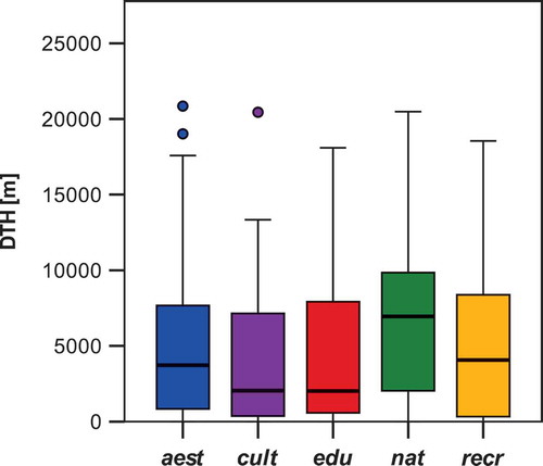
Against this background, it can be argued that the high standard deviation is explained by the methodological design favoring outliers. However, the individual CES (Figure 7) differed significantly (p < 0.0001) in terms of the DTHs. In order to account for the outliers, the median values were considered as critical distances: nat 7 km, cult and edu 2 km, aest and recr 4 km. All districts within these critical distances were assumed to benefit from the services provided by these areas.

3.4. Spatial characterization of the urban region – linking supply and demand

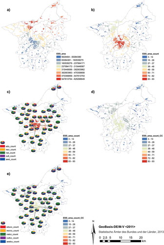
In this section, the results concerning the spatial characterization of the supply of CES (cf. Section 3.1, Figure 5) were linked to the demand of the individual districts (cf. Figure 1b) through the derived critical distances (cf. Section 3.3). Figure 8a illustrates the accumulated area of all CES within the critical distance to the particular districts. Hot-spots could be identified at the coast and within the Rostocker Heide in the north, whereas the city center represented a cold-spot. Thus, the districts with the highest population density seem to be undersupplied with respect to the total area of CES. Figure 8b illustrates the accumulated number of CES areas within the critical distance. Here, the city center represented a hot-spot, whereas the northern city districts were in the mid-range and the rural areas represented cold-spots. Comparing Figure 8a and b, the results suggested that the demand of the population in the city center was not covered by large service areas but by many small ones, as the satisfaction with supply was high in the whole urban region (cf. Section 3.2). To complement these findings, the service diversity is depicted in Figure 8c. The results showed that all the aforementioned hot-spots in terms of CES total area and number were supplied with the maximum diversity of CES (five different ones). As such, diversity hot-spots were in Warnemünde, the Rostocker Heide, and the city center, but included also the main settlements west of the Warnow. Moreover, rural districts, for example, in the northwest on the coast and south of the city center, were dominated by nat services, but to a smaller extent had areas of all other CES within the critical distance, thus still allowing access to the full diversity of services. Other more rural districts were often characterized by a lack of edu and cult services.

Figure 8. Spatial link of supply and demand accumulated for all cultural ecosystem services. (a) The supply area of ecosystem services within the critical distances to the districts (demand). (b) Number of areas within the critical distances. (c) Diversity of the individual cultural ecosystem services (see legend) illustrated by pie charts per district. (d) Number of areas within the critical distances excluding areas of perceived vulnerability. (e) Diversity of the individual cultural ecosystem services excluding areas of perceived vulnerability.

3.5. Integrated vulnerability assessment

The participatory mapping of the perceived vulnerability (Figure 5f) resulted in 12 entries for drought, 61 for heat wave, and 63 after an event of extreme precipitation. The areas of perceived vulnerability largely overlap with the CES identified, thus 40–70% of the CES areas are avoided during or after an extreme event (Hagemeier-Klose et al. 2014). The remaining CES area (Figure 4) suggests a vulnerability in terms of a decreased CES supply.

The comparison of the integrated CES supply–demand map (Figure 8b) and the map corrected according to perceived vulnerability (Figure 8d) revealed considerable differences. The results implied that the potential loss of CES supply areas would affect the city center and the main settlements the most in terms of the number of CES areas within the critical distance. The districts on the coast showed only a slight decline. Looking at service diversity (Figure 8e), the same conclusion could be drawn. The population on the coast, especially in Warnemünde and the Rostocker Heide, seems not to be vulnerable, whereas the population located in the city center and main settlements seems to be vulnerable with regard to a loss of CES areas and in most cases service diversity.

4. Discussion

In this section, the previous thematic structure is retained including CES supply, the categorical link, the spatial link, the integrated demand–supply, and the exemplary vulnerability assessment. The first part presents an in-depth discussion of the methodological approaches including shortcomings and potential improvement. In the second part, the case study results are discussed.

4.1. Method reflection

As in the studies of Fagerholm et al. (2012) and Brown et al. (2012), the participatory mapping approach proved to be a valuable tool defining areas which supply ecosystem services. However, most of these studies were conducted either in developing countries (Fagerholm et al. 2012) or in rural areas (e.g., nature reserve in Brown et al. 2012). Urban areas were seldomly assessed using a participatory mapping approach and, in most cases, the study area was restricted to urban blue and green spaces, as, for example, in Ståhle (2006). The case study presented here showed that an application of the method to a wide urban region comprising an area of over 500 km² is also valuable. Nevertheless, it needs to be acknowledged that due to the participatory approach the term ecosystem service might not be accurate for some of the areas delineated. It may very well be the case that some areas only relate to built-up structures and thus not directly to ecosystem processes. To exemplify, especially for the point data, participants delineated individual houses, for example, a church for spiritual/religious values. One could argue that these areas should be excluded from the analysis. However, ground truthing would be needed to ensure that the value was not related to, for example, green area in front of a build-up structure. This is essentially a problem of scale frequently reported in ecosystem service studies (Alberti 2005; Burkhard, Petrosillo, et al. 2010; De Groot et al. 2010).

The presented study underlines the proposed potential of participatory approaches to assess the CES and their contribution to wellbeing (Maynard et al. 2011; Koschke et al. 2012). The approach was extended by adding the factor of satisfaction to the ranking exercise. This turned out to be valuable variable to reflect results (e.g., DTH). The finding that satisfaction and importance for wellbeing did not relate to the number and size of CES areas mapped by the participants, could be useful for future participatory approaches. For the urban region of Rostock, the rankings for wellbeing and satisfaction were generally high. Thus, although the Likert scale is recommended (Koschke et al. 2012), a very narrow range of results was derived. Retrospectively, I would suggest to use a finer scale for the ranking, in order to be able to evaluate the differences in the higher value field statistically. The high-ranking results could be explained on the one hand by a positive bias because citizens were proud of their own region, which would apply for the majority of participatory mapping approach. On the other hand, this could be related to participant bias, as most of the participants had a higher level of education and socioeconomic class, thus might in general be more satisfied. However, it is difficult to reach other social groups with such participatory approaches.

In order to assess the spatial link between supply and demand of CES, an explorative application of the factor DTH was shown. The different interpretative dimensions were touched upon in the results (cf. Section 3.3). Despite the methodological difficulties (e.g., high standard deviation) that arose, I would like to emphasize the development potential of using this indicator to reveal an integrated CES supply–demand map. The calculation of the DTH could be further developed using not only the direct Euclidian distance but also the Manhattan distance in order to take account of actual accessibility through, for example, the network of roads, paths. However, the presented case study assessed solely the location of the CES areas and their value, not how the participants got there. In consequence, it was not possible to consider the temporal aspects of traveling or issues of accessibility. With the use of the Euclidian distance all traveling possibilities (whether pedestrian, bicycle, public transport, or car) were treated the same way. This decision was supported by the fact that the DTH mean and maximum values did not differ between participants who owned cars and those who did not.

The different DTHs served as an input for the integrated illustration of the CES supply and demand. In addition, the supply per person could be calculated. Moreover, it would also be possible to use this method the other way around. This would enable us to indicate pressure arising from the population demand as done by Palomo et al. (2012) using areas of CES supply as an output system. It should be mentioned that there is a methodological shortcoming related to the boundaries of the overall study area. The results for the outer rural districts are not as reliable as those for the city, since these districts are potentially supplied by CES areas outside the study area. Local characteristics are essential to understand dynamics in social–ecological systems, however, the findings of this case study regarding the categorical and the spatial link between supply and demand are limited to CES.

Data in terms of perceived vulnerability are often demanded (Adger 2006; Hinkel 2011), but have rarely been assessed. One example was shown by Raymond et al. (2009) in the context of threats to ecosystem services assessed via interviews. Here, the data on perceived vulnerability to drought, heat wave, and extreme precipitation were used as exposure variable. Therewith, the case study is restricted to the indication of today’s vulnerability. However, the presented method allowed the visualization of the vulnerability of both the CES supply areas and impacts on the demand side. Moreover, as reported in Hagemeier-Klose et al. (2014) the participatory process initiated learning processes for both scientists and participants uncovering local characteristics of CES and vulnerability.

4.2. Characterizing the urban region

The supply–demand approach is a current development that visualizes both social demands in terms of population density and needs (e.g., energy demand) and the ecosystem’s capacity to provide these services (Burkhard, Kroll, et al. 2010). Following this approach, the results shown in Figure 5 allowed for a characterization of the study area, identifying areas of CES supply and areas of demand considering population distribution. In studies on ecosystem services, the group of CES is often underexplored due to their subjective nature (Chan et al. 2012). In an attempt to close this research gap, the case study demonstrated a method that could give insights into the analysis of CES. The presented CES maps could help to identify which areas are actually used by the population. Results in this context could contribute to planning procedures, for example, by comparing areas planned for recreation and areas actually used for recreation. In addition, the CES hot-spots identified could give implications in terms of what is important for the wellbeing of the local population. Moreover, the CES supply maps indicated an interdependency between the city and its hinterland. This rural–urban dependency has been reported, for example, for the rural energy supply and the urban energy demand (Kroll et al. 2012). Especially for edu and cult, many small CES areas were found in the city center, suggesting that with regard to CES the rural–urban interdependency could be two-sided. Furthermore, it was found that the different CES overlap, indicating that there are no substantial trade-offs between the individual CES, a finding that requires further analysis going beyond the scope of this article. In this context, the focus on CES represents an important limitation of the case study, as an additional comparison to other ecosystem service groups, such as regulating services and an assessment of potential synergies and trade-offs (Haase et al. 2012; Kandziora et al. 2013), would be very interesting.

Although, differences according to social factors were often assumed (Daily et al. 2009), the contribution of ecosystem services to the wellbeing of different social groups is rarely assessed. The presented study developed and tested a method to address these issues. The case study revealed that for all CES the importance for wellbeing as well as the satisfaction with supply was generally high. The high satisfaction rankings are supported by the findings of the perception study concerning the quality of life in cities by the European Commission (2013) for the city of Rostock. The fact, that importance for wellbeing was rated somewhat higher than satisfaction, suggested that enhancement is possible in the urban region. The highest ratings in terms of importance for wellbeing were found for recr. It was however interesting to discover that nat was valued as of equal importance with recr. Complementing these findings with a study on, for example, regulating ecosystem services could have implications for planning in this region by means of synergies.

The extensive survey included 16 different social factors. Nevertheless, no relevant differences for social factors in terms of importance for wellbeing could be identified. However, it needs to be acknowledged that only one aspect of wellbeing, the subjective one, was assessed, showing no differences for social factors. When it comes to, for example, basic human needs (Summers et al. 2012), probably a completely different picture would be revealed. Furthermore, there is a chance that the overall high rankings obscured differences according to social factors. These differences could evoke in case of a shortage in ecosystem service supply.

With the calculation of the DTH, it was possible to establish a spatial link between the supply and the demand of CES. The results revealed no differences in DTH according to social factors. However, critical distances could differ with respect to the other dimensions of wellbeing. The case study included participants ranging in age from 23 to 72 years, which showed no correlation to DTH. It could well be that older people aged 75 plus or especially children have different demands related to critical distances. The concept of using critical distances also considering social factors is not new to the planning process. For example, distances to recreation grounds, which are differentiated into age groups according to the German DIN 18,034 (Agde & Hünnekes 2013). Furthermore, reference values are applied in planning procedures, as in Munich, where the city districts should contain 7 m² open space per resident within 1 km distance (München 2005). Insights from the case study suggesting that the population demands nat areas within a distance ranging from 7 km to no more than 13 km away from the city districts could be further studied to complement these values. Taking into account distances to other CES such as cultural heritage/identity, aesthetics, and education could significantly enhance the planning procedure toward a more comprehensive approach for human wellbeing.

The case study suggested that CES are in general an important factor for the subjective wellbeing of the overall population, with no differences between the population of the city and the hinterland. In addition, both participants from the rural areas and from the city were equally satisfied with the provision of CES. Thus, it could be assumed that not only the supply in terms of the total area of CES but also number of areas and the diversity of CES supply are important for the wellbeing and satisfaction in the urban region.

The characterization of the case study region in terms of the categorical and the spatial link between supply and demand of CES formed the basis for the exemplary vulnerability assessment. The areas of perceived vulnerability seemed equally distributed in the city and its hinterland, however, the same hot-spots were identified as for the CES supply areas. From the spatial analysis of the overlap between CES supply and perceived vulnerability, it was possible to conclude for which CES areas the benefit is lost in case of extreme events. Through the integrated approach, these findings were complemented by the impacts on the CES demand. The results suggested that with regard to a potential loss of CES areas and diversity, the city districts could be more vulnerable than the coastal and rural areas. Vulnerability assessments are often limited to the identification of areas with an urgent need for action, but this information often cannot simply be translated into practical measures (Patt et al. 2005). In contrast, ecosystem service assessments provide information that can be directly used to set up measures to increase specific services as necessary. The method for an integrated vulnerability assessment presented here could be used to identify areas of opportunity with regard to districts that are undersupplied, potential development areas within a critical distance, and the importance of CES for the wellbeing of the population.

5. Conclusions

To evaluate the link between ecosystem services supply and demand integrating social factors and spatial interrelations, participatory mapping proved to be a valuable tool to assess CES and the data needed for analysis. Interestingly, for both the spatial and the categorical link no relevant differences according to social factors could be found. Certainly, studies on other ecosystem services are needed to verify and complement the findings of the case study. However, methodological implications such as the proposed ranking on satisfaction with supply to complement importance for wellbeing and to reflect findings and the potential of assessing critical distances for individual CES could support future studies. Here, nat was valued as of equal importance with recr showing the potential applicability in urban planning identifying synergies. The development of integrated supply–demand visualizations has the potential to facilitate the management of ecosystem services and thus a more comprehensive approach to human wellbeing in urban planning, as it enables the identification of districts that are undersupplied as well as areas that are of importance for the wellbeing of the population. The final exemplary vulnerability assessment showed the potential of the method visualizing both the potential impact on the demand and the supply side. On this basis, climate-change adaptation measures could be discussed with ecosystem services acting as a common language.

Disclosure statement

No potential conflict of interest was reported by the author.

Supplemental data

Supplemental data for this article can be accessed at http://dx.doi.org/10.1080/21513732.2015.1059891.

Acknowledgements

The author is grateful to the participants of the participatory mapping exercise who devoted their time to the process. The author thanks the Research Group Plan B:altic for the ongoing discussions. Special thanks are due to M. Hagemeier-Klose for the help in the organization and performance of the mapping exercise and M. Nagel for the help in GIS processing and layout. I would also like to thank the reviewers for their valuable input.

Additional information

Funding

This work was supported by the HafenCity University Hamburg and the German Federal Ministry of Research and Education through the Social-Ecological Research Program [FKZ 01UU0909].

References

- Adger WN. 2006. Vulnerability. Glob Environ Chang. 16:268–281.
- Agde G, Hünnekes HDA. 2013. Spielplätze und Freiräume zum Spielen: ein Handbuch für Planung und Betrieb. Beuth: Deutsches Institut für Normung e.V.
- Alberti M. 2005. The effects of urban patterns on ecosystem function. Int Reg Sci Rev. 28:168–192.
- Beichler SA, Davidse BJ, Deppisch S 2012. Dynamics of a social-ecological system under climate change – searching for a match with levels of governance. Paper presented at the European Urban Research Association (EURA) Conference “Urban Europe – Challenges to meet the Urban Future”; Sep 20–22; Vienna, Austria.
- Brown G, Montag JM, Lyon K. 2012. Public participation GIS: a method for identifying ecosystem services. Soc Nat Resour. 25:633–651.
- Brown G, Reed P. 2012. Social landscape metrics: measures for understanding place values from public participation geographic information systems (PPGIS). Landsc Res. 37:73–90.
- Bryan BA, Raymond CM, Crossman ND, Macdonald DH. 2010. Targeting the management of ecosystem services based on social values: where, what, and how? Landsc Urban Plan. 97:111–122.
- Burkhard B, Kroll F, Müller F, Windhorst W. 2010. Landscapes’ capacities to provide ecosystem services – a concept for land-cover based assessments. Landsc Online. 15:1–22.
- Burkhard B, Kroll F, Nedkov S, Müller F. 2012. Mapping ecosystem service supply, demand and budgets. Ecol Indic. 21:17–29.
- Burkhard B, Petrosillo I, Costanza R. 2010. Ecosystem services – bridging ecology, economy and social sciences. Ecol Complex. 7:257–259.
- Chan KM, Satterfield T, Goldstein J. 2012. Rethinking ecosystem services to better address and navigate cultural values. Ecol Econ. 74:8–18.
- Crossman ND, Burkhard B, Nedkov S, Willemen L, Petz K, Palomo I, Drakou EG, Martín-Lopez B, McPhearson T, Boyanova K, et al. 2013. A blueprint for mapping and modelling ecosystem services. Ecosyst Serv. 4:4–14.
- Daily GC, Polasky S, Goldstein J, Kareiva PM. 2009. Ecosystem services in decision making: time to deliver. Front Ecol Environ. doi:10.1890/080023
- Daniel TC, Muhar A, Arnberger A, Aznar O, Boyd JW, Chan KMA, Costanza R, Elmqvist T, Flint CG, Gobster PH, et al. 2012. Contributions of cultural services to the ecosystem services agenda. Proc Natl Acad Sci. 109:8812–8819.
- De Chazal J, Quetier F, Lavorel S, Vandoorn A. 2008. Including multiple differing stakeholder values into vulnerability assessments of socio-ecological systems. Glob Environ Chang. 18:508–520.
- De Groot RS, Wilson MA, Boumans RMJ. 2002. A typology for the classification, description and valuation of ecosystem functions, goods and services. Ecol Econ. 41:393–408.
- De Groot RSS, Alkemade R, Braat L, Hein L, Willemen L. 2010. Challenges in integrating the concept of ecosystem services and values in landscape planning, management and decision making. Ecol Complex. 7:260–272.
- Ernstson H. 2013. The social production of ecosystem services: a framework for studying environmental justice and ecological complexity in urbanized landscapes. Landsc Urban Plan. 109:7–17.
- European Commission. 2013. Quality of life in cities – perception survey in 79 European cities. Luxembourg: European Union. doi:10.2776/79403
- [EEA] European Environment Agency. 2009. Ensuring quality of life in Europe’s cities and towns. Copenhagen: European Environment Agency. doi:10.2800/11052
- Fagerholm N, Käyhkö N. 2009. Participatory mapping and geographical patterns of the social landscape values of rural communities in Zanzibar, Tanzania. Fennia. 187:43–60.
- Fagerholm N, Käyhkö N, Ndumbaro F, Khamis M. 2012. Community stakeholders’ knowledge in landscape assessments – mapping indicators for landscape services. Ecol Indic. 18:421–433.
- Gasper R, Blohm A, Ruth M. 2011. Social and economic impacts of climate change on the urban environment. Curr Opin Environ Sustain. 3:150–157.
- Granek EF, Polasky S, Kappel CV, Reed DJ, Stoms DM, Koch EW, Kennedy CJ, Cramer LA, Hacker SD, Barbier EB, et al. 2010. Ecosystem services as a common language for coastal ecosystem-based management. Conserv Biol. 24:207–216.
- Haase D, Schwarz N, Strohbach M, Kroll F, Seppelt R. 2012. Synergies, trade-offs, and losses of ecosystem services in urban regions: an integrated multiscale framework applied to the Leipzig- Halle Region, Germany. Ecol Soc. 17: 22.
- Hagemeier-Klose M, Beichler SA, Davidse BJ, Deppisch S. 2014. The dynamic knowledge loop: inter-and transdisciplinary cooperation and adaptation of climate change knowledge. Int J Disaster Risk Sci. 5:21–32.
- Hermann A, Schleifer S, Wrbka T. 2011. The concept of ecosystem services regarding landscape research: a review. Living Rev Landsc Res. 1:1–37.
- Hinkel J. 2011. ‘Indicators of vulnerability and adaptive capacity’: towards a clarification of the science–policy interface. Glob Environ Chang. 21:198–208.
- Hunt A, Watkiss P. 2011. Climate change impacts and adaptation in cities: a review of the literature. Clim Change. 13–49. doi:10.1007/s10584-010-9975-6.
- Hutton CW, Kienberger S, Amoako Johnson F, Allan A, Giannini V, Allen R. 2011. Vulnerability to climate change: people, place and exposure to hazard. Adv Sci Res. 7:37–45.
- [IPCC] Intergovernmental Panel on Climate Change. 2012. Managing the risks of extreme events and disasters to advance climate change adaptation. A special report of working groups I and II of the Intergovernmental Panel on Climate Change. Cambridge (UK): Cambridge University Press.
- Kandziora M, Burkhard B, Müller F. 2013. Interactions of ecosystem properties, ecosystem integrity and ecosystem service indicators—a theoretical matrix exercise. Ecol Indic. 28:54–78.
- Koschke L, Fürst C, Frank S, Makeschin F. 2012. A multi-criteria approach for an integrated land-cover-based assessment of ecosystem services provision to support landscape planning. Ecol Indic. 21:54–66.
- Kroll F, Müller F, Haase D, Fohrer N. 2012. Rural–urban gradient analysis of ecosystem services supply and demand dynamics. Land Use Policy. 29:521–535.
- Larondelle N, Haase D. 2013. Urban ecosystem services assessment along a rural–urban gradient: a cross-analysis of European cities. Ecol Indic. 29:179–190.
- Martínez-Harms MJ, Balvanera P. 2012. Methods for mapping ecosystem service supply: a review. Int J Biodivers Sci Ecosyst Serv Manag. 8:17–25.
- Maxim L, Spangenberg JH 2003. Bridging the gap between two analytical frameworks. Paper presented at Ninth Biennial Conference of the International Society for Ecological Economics ‘Ecological Sustainability and Human Well-Being’; Dec 15–18; New Delhi; p. 1–20.
- Maynard S, James D, Davidson A. 2011. An adaptive participatory approach for developing an ecosystem services framework for South East Queensland, Australia. Int J Biodivers Sci Ecosyst Serv Manag. 7:182–189.
- [MEA] Millennium Ecosystem Assessment. 2005. Ecosystems and human well-being : millennium Ecosystem Assessment. Washington (DC): Island Press.
- München. 2005. Grünplanung in München. Landeshauptstadt München: Referat für Stadtplanung und Bauordnung, Abteilung Grünplanung.
- Niemelä J, Saarela S-R, Söderman T, Kopperoinen L, Yli-Pelkonen V, Väre S, Kotze DJ. 2010. Using the ecosystem services approach for better planning and conservation of urban green spaces: a Finland case study. Biodivers Conserv. 19:3225–3243.
- Palomo I, Martín-López B, Potschin M, Haines-young R, Montes C. 2012. National parks, buffer zones and surrounding lands: mapping ecosystem service flows. Ecosyst Serv. 4:1–13.
- Patt A, Klein RJT, de la Vega-Leinert A. 2005. Taking the uncertainty in climate-change vulnerability assessment seriously. Comptes Rendus Geosci. 337:411–424.
- Plieninger T, Dijks S, Oteros-Rozas E, Bieling C. 2013. Assessing, mapping, and quantifying cultural ecosystem services at community level. Land Use Policy. 33:118–129.
- Preston BL, Yuen EJ, Westaway RM. 2011. Putting vulnerability to climate change on the map: a review of approaches, benefits, and risks. Sustain Sci. 177–202. doi:10.1007/s11625-011-0129-1
- Radford KG, James P. 2013. Changes in the value of ecosystem services along a rural-urban gradient: a case study of Greater Manchester, UK. Landsc Urban Plan. 109:117–127.
- Raymond CM, Bryan BA, MacDonald DH, Cast A, Strathearn S, Grandgirard A, Kalivas T. 2009. Mapping community values for natural capital and ecosystem services. Ecological Econ. 68:1301–1315.
- Rounsevell MDA, Dawson TP, Harrison PA. 2010. A conceptual framework to assess the effects of environmental change on ecosystem services. Biodivers Conserv. 19:2823–2842.
- Schulp CJE, Lautenbach S, Verburg PH. 2014. Quantifying and mapping ecosystem services: demand and supply of pollination in the European Union. Ecol Indic. 36:131–141.
- Sherrouse BC, Clement JM, Semmens DJ. 2011. A GIS application for assessing, mapping, and quantifying the social values of ecosystem services. Appl Geogr. 31:748–760.
- Ståhle A. 2006. Sociotope mapping – exploring public open space and its multiple use values in urban and landscape planning practice. Nord J Archit Res. 19:59–71.
- Stürck J, Poortinga A, Verburg PH. 2014. Mapping ecosystem services: the supply and demand of flood regulation services in Europe. Ecol Indic. 38:198–211.
- Summers JK, Smith LM, Case JL, Linthurst RA. 2012. A review of the elements of human well-being with an emphasis on the contribution of ecosystem services. Ambio. 327–340. doi:10.1007/s13280-012-0256-7
- Syrbe R-U, Walz U. 2012. Spatial indicators for the assessment of ecosystem services: providing, benefiting and connecting areas and landscape metrics. Ecol Indic. 21:80–88.
- Turner BL, Kasperson RE, Matson PA, McCarthy JJ, Corell RW, Christensen L, Eckley N, Kasperson JX, Luers A, Martello ML, et al. 2003. A framework for vulnerability analysis in sustainability science. Proc Natl Acad Sci U S A. 100:8074–8079.