Comparison of methods for a landscape-scale assessment of the cultural ecosystem services associated with different habitats

ABSTRACT

Cultural ecosystem services (CES) are widely acknowledged as important but are often neglected by ecosystem service assessments, leading to a representational bias. This reflects the methodological challenges associated with producing robust and repeatable CES valuations. Here we provide a comparative analysis of three approaches for non-monetary valuation of CES, namely a structured survey, participatory GIS (PGIS) and GPS tracking methods. These were used to assess both recreation and aesthetic value of habitats within the New Forest National Park, UK. The association of CES with habitats enabled results of all three methods to be visualised at the landscape scale using maps, strengthening their value to conservation management. Broadleaved woodland and heathland habitats were consistently valued highly for both CES, whereas agricultural land tended to be associated with low values. Results obtained by the different methods were positively correlated in 6 out of 10 comparisons, indicating a degree of consistency between them. The spatial distribution of CES values at the landscape scale was also generally consistent between the three methods. These results highlight the value of comparative analyses of CES for identifying robust results, providing a way forward for their inclusion in land management decision-making.

EDITED BY Matthias Schröter

KEYWORDS:

• CES
• cultural ecosystem services
• PGIS
• surveys
• behaviour
• stated preference
• recreation

Edited by Matthias Schröter

1. Introduction

Growth in adoption of ecosystem services as a policy concept has been accompanied by a rapid increase in research effort, which has documented the factors influencing the provision of ecosystem services in a wide range of ecosystems and socio-economic contexts (Carpenter et al. 2009; Nicholson et al. 2009; Seppelt et al. 2011). However, relatively little progress has been made in assessing cultural ecosystem services (CES), which are often neglected owing to methodological challenges (Feld et al. 2009; Seppelt et al. 2011; Daniel et al. 2012; Plieninger et al. 2013). This has led to a representational bias in ecosystem assessments and landscape planning decisions, in which CES are often poorly represented (Hernández-Morcillo et al. 2013). CES are often referred to as ‘intangible’ and ‘subjective’, reflecting the difficulties associated with their quantitative assessment and valuation (Millennium Ecosystem Assessment (MEA) 2005; Daniel et al. 2012). Despite such difficulties, the importance of CES has widely been acknowledged. For example, Guo et al. (2010) found that the dependence of people on cultural services increased as economic development took place, often exceeding that of regulating services. CES have also been found to be important motivators for land management and ownership (Plieninger et al. 2012). Increasingly, CES are being embedded in environmental decision-making at a range of geographical and temporal scales, with the aim of achieving ecological sustainability, social justice and economic efficiency in an integrated way (Costanza et al. 2017).

CES represent a very diverse group of ecosystem services, and consequently a wide range of methods have been employed in their assessment and valuation (Milcu et al. 2013; Hirons et al. 2016). Factors such as social and cultural background, habits and belief systems, behavioural traditions and lifestyles can have a major influence on CES values, and many studies have adopted methods involving qualitative assessment of individual perceptions. The results obtained with such approaches are difficult to verify, however (Hernández-Morcillo et al. 2013). The lack of robust approaches to valuing CES may account for the fact that they are often neglected in practical assessments (Hernández-Morcillo et al. 2013; Milcu et al. 2013; Hirons et al. 2016). For example, in a meta-analysis of 524 quantitative indicators of biodiversity and ecosystem services from 89 restoration assessments, Rey Benayas et al. (2009) found no studies that measured cultural services explicitly. While an increasing number of investigations valuing CES have been published since this study, no consensus has emerged regarding which methods are most consistent or robust (Costanza et al. 2017).

In part, the methodological challenges of assessing CES values stem from conceptual uncertainty regarding the nature of CES, and how the provision of these benefits is related to the characteristics and condition of ecosystems (Fish et al. 2016). In many studies, socio-cultural values are assumed to be linked to ecological functions and structures, yet this may obscure conflicts regarding the conflation of ‘nonmaterial’ values with more tangible benefits of CES (Stålhammar and Pedersen 2017). For example, Fraser et al. (2016) suggested that for a genuinely holistic approach to valuation of CES, methods may need to be drawn not only from natural and quantitative social sciences but also from interpretivist qualitative social science and humanities, located within a suitable theoretical framework such as phenomenology. However, this would be difficult to achieve within a single analytical framework. In a critique of the CES concept, James (2015) goes further, and suggests that even if approaches such as phenomenology or textual analysis were used, they would nevertheless be reinterpreted in terms of service provision. This would fail to capture the full value of places to people’s lives, including historical, political, mythic and spiritual values. Furthermore, the processes and characteristics that underpin provision of CES may be difficult to observe and measure, and may not directly be linked with features of ecosystems that can be readily assessed (Fish et al. 2016).

As a result of such issues, the valuation of CES presents a significant challenge to achieving a genuinely holistic ecosystems approach to decision-making (Fish et al. 2016). The under-representation of CES in ecosystem service assessments could potentially lead to biases in landscape planning and management, in which the needs of users of a particular area are neglected (Hernández-Morcillo et al. 2013). Potentially, comparative analysis of different approaches for valuing CES could help verify the results obtained, and thereby strengthen the process of CES assessment. In practice, very few previous studies have performed such comparisons; this issue was largely ignored by recent reviews of CES (Hernández-Morcillo et al. 2013; Milcu et al. 2013; Hirons et al. 2016). Yet the use of different methods to cross-check and validate results is widely acknowledged to be an important contributor to strengthening the development of other types of environmental indicators (Niemi and McDonald 2004). Results that are consistently obtained by different methods could be considered to be relatively robust, whereas those findings that differ between methods suggest areas of relative uncertainty.

Here, we examine recreation and aesthetic value as examples of CES (Costanza et al. 1997; De Groot et al. 2002), as efforts to value non-material benefits of ecosystem services usually focus on these services as they have tangible benefits (Milcu et al. 2013; Baulcomb et al. 2015; Small et al. 2017). De Groot et al. (2010) define aesthetic value as being the appreciation of natural scenery (other than through deliberate recreational activities), with recreational value being defined as the opportunities for tourism and recreational activities. We examine these services in relation to the distribution of different habitats at the landscape scale. Much conservation management and policy focuses on maintaining or improving the condition of habitats, as illustrated for example by the EU Habitats Directive in Europe. While habitat management interventions aimed at biodiversity conservation may provide multiple co-benefits for provision of ecosystem services, more information is needed on where these synergies occur in order to realise such benefits (Austin et al. 2016). Furthermore, where the primary management focus is on provision of ecosystem services, as in Ecosystem-Based Management, analysis of both synergies and trade-offs will be required to ensure win-win outcomes for both biodiversity and human society (Ingram et al. 2012; Cordingley et al. 2015).

In order for the factors influencing provision of CES to be understood, and the management of CES to be optimised at the landscape scale, the spatial and temporal dynamics of CES need to be analysed. While a wide range of different methods have been used for valuing CES (Hirons et al. 2016), no consensus has been reached regarding the appropriate choice of method for assessing CES at the landscape scale (Seppelt et al. 2011; Hernández-Morcillo et al. 2013). While both monetary and non-monetary valuation methods can potentially be used (Hirons et al. 2016), here we focus on the latter, reflecting the fact that monetary valuation of CES is often not deemed appropriate (Milcu et al. 2013). We compare three different methods: a stated preference survey, participatory Geographical Information Systems (PGIS), and use of Global Positioning System (GPS) trackers, to assess the relative value of different habitats for provision of CES at the landscape scale.

Many previous studies of CES have used stated-preference methods; for example, Newton et al. (2012) in the River Frome, Dorset, Southern England, and Barrena et al. (2014) in Chiloé Island, southern Chile. These methods can be divided into two main groups: contingent valuation and choice modelling techniques. Contingent valuation surveys ask participants their ‘willingness to act’ or ‘willingness to pay’ for changes, whereas choice modelling surveys present participants with several alternatives and elicit preference values from them (Riera et al. 2012). Surveys are typically designed so that the answers to the questions can be designed as a choice experiment, contingent ranking, rating or grouping (Brown 2003; Riera et al. 2012).

PGIS methods are computer-based mapping approaches that involve members of the community (Abbot et al. 1998; Dunn 2007), and are becoming increasingly popular for mapping ecosystem services, especially CES (Milcu et al. 2013; Brown and Fagerholm 2015). PGIS can range from simple paper-based approaches to more complex online maps (Brown et al. 2012). Examples include mapping social values in Helsinki, Finland for strategic green area planning (Tyrväinen et al. 2007), supporting coral reef ecosystem management in Hawaii (Levine and Feinholz 2015) and to support management of the Chugach National Forest, Seward, AK, USA (Brown and Reed 2000). Such examples have highlighted the value of the technique for strengthening stakeholder identification and engagement, and for helping land managers to understand the potential impacts of their decisions on human communities (Dunn 2007).

There are various methods that can be used to directly survey movement patterns of people in an area. These include use of field observations, self-registration approaches, video cameras, GPS trackers, smartphones, social media derived information (e.g. twitter feeds) and thermal cameras (Deadman and Gimblett 1994; O’Connor et al. 2005; Lau and McKercher 2006; Shoval and Isaacson 2007; Garthe 2010; Pettersson and Zillinger 2011; Birkin and Malleson 2012; Orellana et al. 2012; Del Rosario et al. 2015). Examples of the application of such methods include use of geo-spatial ankle transmitters on visitors to Twelve Apostles National Park in Victoria, Australia, to determine tourist behaviours (O’Connor et al. 2005), and use of large GPS data sets to discover commonalties of visitor preferences in natural recreational areas (Orellana et al. 2012). Previous research utilising geo-tagged images has been used to ascertain recreation preferences for habitats (Oteros-Rozas et al. 2017), though no previous studies have used continuous GPS-tracking approaches for assessing human movement patterns in relation to CES values associated with different habitats.

We examine these services at the landscape scale, as despite the widespread use of these different methods, few studies have been undertaken of their relative performance, specifically in relation to assessment of CES at this scale (Milcu et al. 2013; Hirons et al. 2016). Such comparisons are needed, both to identify the extent to which survey results are dependent on the method used, and because the methods vary in regard to their technical requirements and relative economic cost. Here, we compared the relative performance of three different assessment approaches for assessing the relative non-monetary value of different habitats for recreation and aesthetic values in the New Forest National Park, UK. This area is a major resource for recreation, attracting over 13 million day visits per year (Sharp et al. 2008). However, little information is available on spatial patterns of visitor movement within this National Park, and how this relates to the spatial distribution of different habitats. Our study complements that of Willcock et al. (2017), who compared three different CES survey methods at a range of sites in southern England, including the New Forest. The survey tools included language-based supervised surveys, language-based unsupervised surveys and image-based unsupervised surveys, which were used to assess the CES values associated with individual sites. Unlike Willcock et al. (2017), our focus is to examine heterogeneity in CES provision within an individual landscape; further, our approach is spatially explicit, to enable the spatial valuation of CES to be integrated into regional planning and development (Tammi et al. 2017).

2. Methods

2.1. Study area

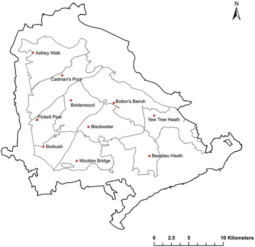
The New Forest National Park covers 56,658 ha on the south coast of England (Lat. 50°51ʹ59ʺ N, Long. 01°40ʹ50ʺ W; see Figure 1) (New Forest Park Authority (NFPA) 2010). Designated in 2005, the New Forest National Park includes 20 SSSIs, six Natura 2000 sites, and two Ramsar Convention sites at least partly within its boundaries. The New Forest Special Area of Conservation (SAC), which forms the core area of the Park, comprises a large number of habitats including broad-leaved deciduous woodland (29%), coniferous woodland (17%) and heath (34%) (JNCC 2011). This complex mosaic of habitats is of relatively high value for biodiversity, with high species richness in groups including insects, birds, mammals, reptiles, fungi and lichens, amongst others (Newton 2010). The topography is gently undulating, and the underlying geology is comprised of gravel terraces, divided by valleys that are filled with clays and sand of Tertiary deposits (New Forest Park Authority (NFPA) 2008).

Figure 1. Map of the New Forest National Park showing management units in grey and surveyed car park locations marked in red (derived from Ordnance Survey data © Crown copyright and database right 2016).

Large populations of free-ranging large herbivores, including cattle, wild deer (fallow, red, roe and sika) and the New Forest Pony, make a significant contribution to the functioning of the New Forest as an ecological system. The Forest originated as a Royal hunting reserve in 1079, and a traditional commoning system involving the depasturing of livestock survives to the present day (Newton 2010). Currently, nearly a quarter of the Park is used for farmland and settlements. Approximately 50% of the Park’s land is covered by unenclosed vegetation, often referred to as the ‘Open Forest’, within which large herbivores are free to roam (New Forest Park Authority (NFPA) 2008; Newton 2010). The New Forest has been a major recreational resource since the mid-nineteenth century, continuing to the present day (New Forest Park Authority (NFPA) 2008). Forty per cent of New Forest visitors are staying tourists, a further 25% are day-trippers travelling from beyond 8 km, whereas locals (living within 8 km) account for 35% of recreational users (Sharp et al. 2008).

2.2. Method 1: stated preference survey

A questionnaire survey was conducted to elicit CES values for different habitats. The questionnaire employed fixed-sum scoring questions (Thomas 2004), which asked a participant to score a set of choices that sum to 100. Participants were asked to score the relative value of each habitat type for both recreation and aesthetic value, by allocating 100 points amongst them. The following habitat types were included: acid grassland, arable cereals, arable horticulture, broad-leaved/mixed woodland, coniferous woodland, dwarf shrub heath, fen/marsh/swamp, improved grassland, neutral grassland, suburban/rural developed and urban. These broad habitat types were selected on the basis of being the most abundant terrestrial habitats in the New Forest. Images of each habitat were provided as a ‘pop-up’ box, to facilitate the understanding of the habitat type. Images were selected as being representative of the local habitats by the authors due to extensive familiarity with the study area. There is potential that the images could have influenced the preference for some habitats, therefore the images were only available to the user if they expressed a lack of understanding of the habitat type by clicking a ‘help’ link. The survey was created as an internet site, which was live between January 2014 and July 2014. Study participants were self-selecting. The survey was promoted in local print, digital media and email aimed at local interest groups, asking for individuals whom resided, worked or used the New Forest National Park.

2.3. Method 2: PGIS

Directly after the questionnaire survey, the same participants from method 1 completed a PGIS survey conducted on the same internet site. A map produced using Google Maps API v3 (Google UK Ltd., London, UK) with the boundary of the New Forest was presented to participants with instructions to place pins on the map. The participant could zoom in and out to select precise locations, but could only place ‘pins’ within the defined boundary of the New Forest. Participants were asked to place ‘pins’ on the map to identify locations of aesthetic and recreational value. Each individual could place up to five pins for each service, and was invited to associate a score with each pin on a Likert scale from 1–5, ranging from least important to most important.

Data were captured in a MySQL database and any responses with missing scores were removed. The latitude, longitude and score for each point were imported into ArcMap 10.1 (ESRI UK Limited, Aylesbury, UK). Point data were projected to British National Grid (OSGB 36) using the Ordnance Survey (OS) OSTN02 transformation (University of Edinburgh 2015). A habitat map (25 x 25 m cell size) for the New Forest provided by Hampshire Biodiversity Information Centre (HBIC, Hampshire County Council, Winchester) was used to extract habitat data for the points.

2.4. Method 3: GPS tracking

Stratified random sampling was used to assess the recreational behaviour of people visiting the New Forest. The Park is divided into 10 management units; each unit was used as an individual sampling stratum. From each, a random car park was chosen from a list extracted from an OS map. Car parks were chosen as sampling points (Figure 1), as previous research has indicated that the majority of visitors to the New Forest (>88%) use a car or private vehicle (New Forest Park Authority (NFPA) 2007). To obtain a representative range of participants, each car park was visited between 08:00 and 18:00, individuals entering the car park were approached in order of entry, until 20 individuals had completed the study at each location. Understanding visitation patterns was not an aim in this study, so set times, days and weather patterns were not taken into account. The same two surveyors were always present during the collection of data. Visitors were approached and invited to participate in the survey, and the study explained to them. If they wished to proceed, a ‘Participant information sheet’ was given to them, and consent form signed.

GPS data loggers were used to track the movement of participants during the recreational visits. The Qstarz BT-Q1000XT trackers used (Qstarz 2013) were small and easily transported, having a belt loop that could be attached to clothing or bags if the participant wished. This method allows for very accurate geospatial information to be collected, including the time that was spent in different areas (Fearnley 2013). This model was selected as compared to six other commercially available GPS units, it showed the smallest mean error (Duncan et al. 2013); it is built with a MTK II GPS module, featuring 66 channels with a sensitivity of −165 dBm, with a stated horizontal accuracy of 3.0 m (Qstarz 2013). The units were set to record the location of a waypoint at set intervals of every 5 s. Habitat classification was subsequently extracted for each waypoint from the HBIC 25m raster to give individual percentage time spent in each habitat type for each participant. The mean for each habitat type was used to calculate normalised values.

2.5. Statistical analysis

Differences between the values associated with each habitat type were determined using Kruskal–Wallis H tests since Kolmogorov–Smirnov testing showed all habitat types chosen by visitors significantly deviated from a normal distribution. Post-hoc pairwise Mann–Whitney tests were used to determine differences between individual pairs of habitats. Spearmans rank correlations were conducted to test the relationships between results obtained with different methods. Both aesthetic and recreation values were normalised prior to analysis. All data analyses were conducted using IBM SPSS Statistics v.22 (IBM United Kingdom Limited, Portsmouth, UK). While the PGIS and GPS tracking methods used the full 22 habitat types present in the New Forest, a reduced number of 9 types were used in the structured survey, as 22 habitats were too many to include in the exercise; the habitats selected were those that were most extensive in the study area (acid grassland, arable and horticulture, broadleaved/mixed/yew woodland, built-up areas and gardens, coniferous woodland, dwarf shrub heath, fen/marsh/swamp, improved grassland and neutral grassland).

3. Results

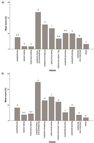
A total of 132 individuals completed the stated preference survey and PGIS task. In the stated preference survey, the distribution of scores was found to be significantly different between habitat types for both recreation (Kruskal–Wallis H test, χ²(10) = 554.531, P < 0.001, two-sided) and aesthetic value (Kruskal–Wallis H test, χ²(10) = 650.326, P < 0.001, two-sided) (Figure 2(a,b)). For recreation, visitors most preferred broadleaved woodland, followed by coniferous woodland and dwarf shrub heath (Figure 2(a)), with arable cereals and arable horticulture least preferred. Similarly, broadleaved woodland was most preferred for aesthetic value. This was followed by dwarf shrub heath and coniferous woodland (Figure 2(b)). The least favoured aesthetically were urban, followed by arable cereals and horticulture areas.

Figure 2. Bar charts illustrating the mean preference for (a) recreation value (b) aesthetic value for habitats, using a survey method. The overall difference between the median ranks of habitats was significant for (b) recreation value and (b) aesthetic value. Bars grouped by the same letter are not significantly different from each other (pairwise comparisons, p < 0.05, without Bonferroni correction).

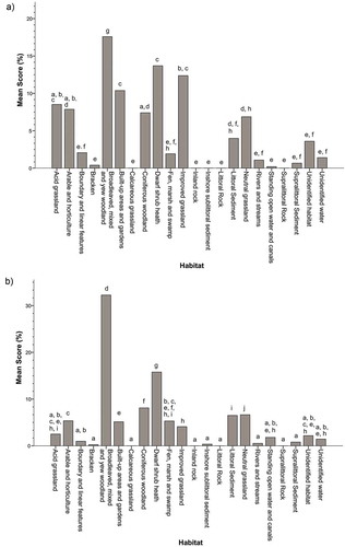
Somewhat similar results were obtained with the PGIS. Broadleaved woodland and dwarf shrub heath were again the habitats most preferred for recreation (Kruskal–Wallis H test, χ²(21) = 309.685, P < 0.001, 2-sided) (Figure 3(a)), although these were followed by improved grassland and built-up areas and gardens, in contrast to the results obtained with the stated preference survey. The lowest scoring habitats, with zero or near zero values, were calcareous grassland, inland rock, inshore sublittoral sediment, littoral rock and supralittoral rock. For aesthetic value, broadleaved woodland was higher than any other habitat, followed by dwarf shrub heath (Kruskal–Wallis H test, χ²(21) = 388.046, P < 0.001, 2-sided) (Figure 3(b)). The habitats with lowest values were calcareous grassland, inland rock, inshore sublittoral sediment, littoral rock and supralittoral rock.

Figure 3. Bar charts illustrating the mean percentage of (a) recreation value and (b) aesthetic value, using participatory GIS. The overall difference between the median ranks of habitats was significant for (a) recreation value and (b) aesthetic value. Bars grouped by the same letter are not significantly different from each other (pairwise comparisons, P < 0.05, without Bonferroni correction).

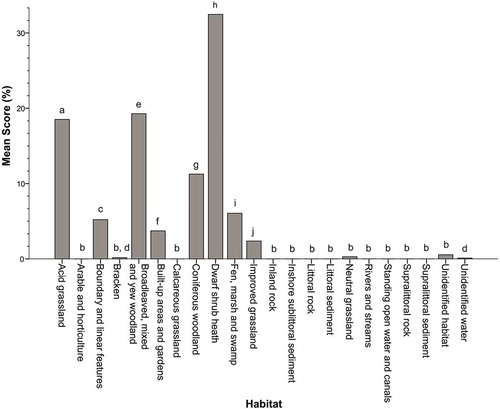
GPS tracking was completed by 200 individuals in total and only used to assess recreation values, and not aesthetic value (Kruskal–Wallis H test, χ²(21) = 1,539.982, P < 0.001, 2-sided) (Figure 4). For recreation, dwarf shrub heath was the most preferred habitat, the next highest being broadleaved woodland and acid grassland. The lowest scoring were littoral and sublittoral habitats, arable and horticulture and calcareous grassland.

Figure 4. Bar chart illustrating the mean percentage of recreation value using GPS tracking. The overall difference between the median ranks of habitats was significant. Bars grouped by the same letter are not significantly different from each other (pairwise comparisons, P < 0.05, without Bonferroni correction).

When values from the three methods were compared, each was found to demonstrate substantial variation among habitat types, with some habitats (such as arable and horticulture, bracken and littoral sediments) consistently recording low values for both services regardless of method (Table 1). We examined whether these results could have been influenced by variation in the area of different habitats within the study area by conducting a Spearman rank correlation. The area of each habitat within the landscape was found to be positively correlated with the recreational values obtained by each of the three methods (P < 0.05 in each case), and the aesthetic value obtained from PGIS (P < 0.01 in each case), providing some support for this hypothesis. However, the low recreational and aesthetic value of arable and horticultural land cannot be attributed to this effect, as it was far greater in extent than a range of other habitats that scored more highly for CES provision (Table 1).

Table 1. Area of habitat types within the study area and the normalised mean (between 0 and 1) value for recreation and aesthetic values for each method utilised.

Habitat	Area (ha)	Recreation			Aesthetic
		Survey	PGIS	GPS tracking	Survey	PGIS
Acid grassland	3167	0.27	0.48	0.57	0.25	0.08
Arable and horticulture	4539	0.00	0.45	0.00	0.06	0.17
Boundary and linear features	387		0.12	0.16		0.03
Bracken	303		0.02	0.01		0.01
Broadleaved, mixed, and yew woodland	14,294	1.00	1.00	0.59	1.00	1.00
Built-up areas and gardens	2583	0.15	0.59	0.12	0.00	0.16
Calcareous grassland	0.13		0.00	0.00		0.00
Coniferous woodland	4949	0.64	0.42	0.35	0.46	0.25
Dwarf shrub heath	9968	0.53	0.78	1.00	0.57	0.49
Fen, marsh and swamp	3030	0.22	0.12	0.19	0.42	0.16
Improved grassland	9924	0.39	0.70	0.07	0.11	0.13
Inland rock	33		0.00	0.00		0.00
Inshore sublittoral sediment	33		0.00	0.00		0.01
Littoral Rock	2.65		0.00	0.00		0.00
Littoral Sediment	1259		0.23	0.00		0.20
Neutral grassland	1030	0.38	0.39	0.01	0.27	0.21
Rivers and streams	1098		0.06	0.00		0.02
Standing open water and canals	79.0		0.01	0.05		0.06
Supralittoral Rock	0.56		0.00	0.00		0.00
Supralittoral Sediment	55.0		0.04	0.00		0.03
Unidentified habitat	1073		0.20	0.02		0.07
Unidentified water	143		0.08	0.00		0.04

Spearman rank correlation analysis (Table 2) showed that there was no correlation between the recreation values obtained by structured survey and those obtained either by PGIS or GPS tracking. However, a significant correlation (P < 0.01, Table 2) was obtained between the recreation values from PGIS and GPS tracking. In contrast, for aesthetic value, results from PGIS and the structured survey were positively correlated (P < 0.05). Aesthetic values obtained from the structured survey were positively correlated with recreational values obtained using the same method, and also with recreational values obtained by GPS tracking. Similarly, both recreational and aesthetic values obtained from PGIS were positively correlated (Table 2).

Table 2. Spearman rank correlations between all methods utilised for recreation and aesthetic value assessment using two-tailed tests. Unity-based normalisation was used on the means for each habitat type for each method before testing. To compare the survey method, the ‘arable cereals’ and ‘arable horticulture’ classes were combined and the classes ‘Urban’ and ‘Suburban rural developed’ were combined. Values in bold are statistically significant.

Method		Recreation			Aesthetic
		Structured survey	PGIS	GPS tracking	Structured survey	PGIS
Recreation	Structured survey	–	r = 0.450 P = 0.224	r = 0.634 P = 0.067	r = 0.817 P < 0.01	r = 0.617 P = 0.077
	PGIS		–	r = 0.757 P < 0.01	r = 0.200 P = 0.606	r = 0.884 P < 0.01
	GPS tracking			–	r = 0.734 P < 0.05	r = 0.659 P < 0.01
Aesthetic	Structured survey				–	r = 0.767 P < 0.05
	PGIS					–

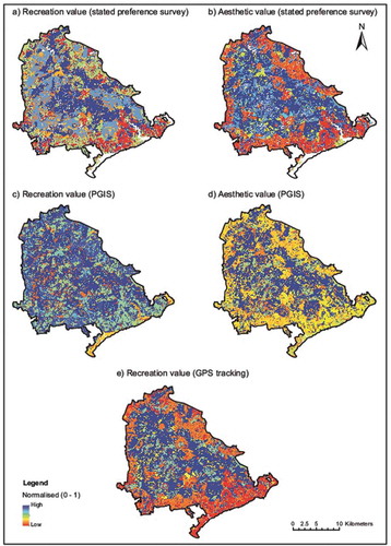
When values were mapped (Figure 5), pronounced spatial variation in both recreational and aesthetic value were observed across the study area, reflecting the spatial distribution of different habitat types. More importantly, the spatial pattern of CES value differed depending on the survey method used. For example, more central areas of the park were associated with higher recreational and aesthetic values than more peripheral areas when values derived from the structured survey were mapped, as the higher scoring habitats are situated nearer the centre of the park. Similar results were obtained for aesthetic value using PGIS, but recreational values obtained from PGIS were not so clearly differentiated. On the other hand, recreational values obtained from GPS tracking showed a clear differentiation between core and peripheral areas of the park; this spatial distribution accorded most closely with the aesthetic values obtained from the structured survey (Figure 5). However, it should be noted that the distribution of car parks that were included in the sample (Figure 1) is higher in the core areas of the park than in the periphery, which may partly account for the results obtained with this method.

Figure 5. Habitat maps based on the Hampshire Biodiversity Information Centre (HBIC) at a 25 × 25m resolution, displaying the normalised mean value for each habitat for recreation value (a, c, e) and aesthetic value (b, d), by method: structured survey (a, b), PGIS (c, d) and GPS tracking (e). Areas shown as white (a, b) were not included in the list of habitats presented to participants for this method, hence have not been included.

4. Discussion

Our results provide a number of insights into the comparative performance of the different methods employed. All three methods captured a wide range of different CES values for different habitats, and provided a means to visualise these values through production of maps. In this respect, each of the methods has potential value in terms of enabling CES to be incorporated into land management planning, in a way that could be integrated with biodiversity conservation. Some findings were consistent among the different methods. For example, broadleaved woodland was repeatedly found to be associated with relatively high values for both recreation and aesthetic value; dwarf shrub heath also scored relatively highly. A number of previous studies have recorded a preference for wooded over more open landscapes in natural and semi-natural systems (Schroeder and Orland 1994; Cordingley et al. 2015), perhaps reflecting a belief that such landscapes are more ‘natural’ in character (Lamb and Purcell 1990). Similarly, the relatively low CES values observed here for agricultural land were also largely consistent between methods, although both arable and improved grassland scored relatively highly with PGIS compared to the other methods. Despite no previous studies comparing these methods for evaluation of CES, results between the three methods were also broadly consistent in terms of the maps produced, for example by highlighting the relatively high value of core areas of the National Park for CES provision.

A lack of correspondence between results obtained by structured survey and GPS tracking for recreation value can be seen. This may be due to the potential limitations of stated preference techniques, as the values obtained might not accurately reflect human behaviour. A tendency for behavioural actions to differ from stated preferences relating to environmental values has been well documented in the environmental psychology literature, where it is referred to as the ‘value-action gap’ or ‘belief-behaviour gap’ (Blake 1999; Godin et al. 2005). While the reasons for this gap remain poorly understood, it has been identified in a number of different contexts relating to environmental decision-making by individuals, and hence it is important that verbal statements without ‘revealed preferences’ not be assumed to reflect ‘manifest interest’ (Klintman 2016). In the current investigation, we sought to address the limitations of stated preference by including direct observation of human use of different habitats using GPS tracking. This enabled stated preference values to be compared with a measure of actual behaviour. As the participants were different between the stated and observed methods, there is the possibility that the behaviour between the groups varied naturally, though self-selection and random sampling in the methods would aid this issue. Results provided little evidence for the value-action gap, as both recreational and aesthetic values for different habitats obtained using structured survey and PGIS techniques were found to be positively correlated with GPS tracking values, with the exception of recreation values elicited with the structured survey. While GPS tracking might be considered superior to the other methods because it involves direct observation of human behaviour, it should be noted that time spent by individuals within a particular habitat does not necessarily relate directly to recreational value. For example, habitats of relatively low value may need to be traversed during a recreational visit to access areas with relatively high value. Positive correlation of GPS tracking recreation values and the extent of habitats suggests that the availability of habitats was a large factor for recreational choice. Though the greater the distance a visitor moved during their visit, the weaker the relationship between habitat availability and preference became (Supplementary materials).

This investigation did not attempt to provide a comprehensive assessment of methods that could be used to assess CES. Many alternative approaches are available that could usefully be considered by future comparative analyses, including text-based approaches, photo-elicitation methods and social media photograph analysis (Hirons et al. 2016). The latter method focuses on analysing the content of crowdsourced, georeferenced photographic data sets, such as Flickr. This approach is employed by the InVEST software tool, which is increasingly being used to conduct ecosystem service assessments worldwide (Sharp et al. 2015). Application of this approach to our study area provided very different results to the other methods presented here. Social media photographs tended to be clustered around urban areas and along roads, suggesting that many visitors to the area upload photographs taken from their vehicles (Supplementary materials). This implies a very biased sample of the study area, which is likely to provide very limited insights into the relative value of different habitats for CES provision. Such observations highlight the potential risks or uncertainties that may be associated with using particular methods in a conservation management context, but also emphasise the value of comparing multiple approaches to strengthen overall rigour.

5. Conclusions

On the basis of the results presented here, which approach should conservation managers adopt to assess CES? We suggest that a focus on evaluating the relative value of different habitats for CES provision might provide a useful way forward. This approach can potentially provide a basis for understanding how specific landscape structures, features or ecosystem properties contribute to CES values, an element that has been little researched in the past (Scholte et al. 2015). Furthermore, each of the methods compared here provide spatially explicit output, which can enable potential changes in CES provision to be identified that might result from conservation management actions. Spatially explicit information about the relationship between CES values and landscape and ecosystem characteristics can help to inform spatial planning and environmental management decisions (Crossman et al. 2013). Our results have highlighted the value of applying multiple methods simultaneously, enabling relatively robust findings to be identified. The diverging results illustrate that different methods address different aspects of CES value, and a pluralistic approach to selection of methods may therefore provide richer insights into the distribution of CES values than use of methods in isolation (Scholte et al. 2015).

Potentially, results obtained by multiple methods could be integrated using GIS, by combining or overlaying data layers. However in practice, we recognise that conservation managers may be limited in terms of the number of CES valuation methods that they are able to deploy. Measuring CES can often prove expensive and time consuming (Church et al. 2014). In this investigation, we did not systematically evaluate the costs associated with implementing the three methods, although the GPS tracking required purchase of specialised equipment and was more labour intensive than the other approaches, and was therefore associated with a higher cost. Other research has found that it is much more cost effective per respondent to have supervised surveys over unsupervised surveys for collecting CES information (Willcock et al. 2017). It should be noted that the issue of comparability of the results from the different methods is of critical consideration. Whereas, the GPS tracking and PGIS methods allow explicit spatial mapping of data, the structured survey assumes that all habitat types will have the same value once mapped. This assumption disregards abiotic and biotic features in the landscape that may influence recreation and aesthetic preferences. The GPS tracking was only used as an indicator of recreation value in this study, though in reality aesthetic appeal would have been a factor in where the participant chose to visit, though it was not possible to differentiate this from the recreation value in the data captured. The positive correlations recorded here between the results obtained by different methods suggest that if resources are limiting, a single method might usefully be deployed. On the basis of the current results, PGIS might be considered the preferred method, on the basis of the most number of correlations recorded with the results of other methods. Our findings therefore support those of other authors who have highlighted the value of PGIS approaches for CES valuation (Hernández-Morcillo et al. 2013; Milcu et al. 2013). It should also be noted that recreational and aesthetic value were in some cases found to be correlated, suggesting that one CES can potentially be used as a proxy for the other. However, such an inference should be made with caution, as these two services are not always correlated, a finding observed both here and by previous research (Cordingley et al. 2015). This reflects the fact that people do not choose recreation opportunities based solely on aesthetic values, but on other criteria such as convenience and accessibility (McShane et al. 2011; Sen et al. 2011).

According to Church et al. (2014), CES can usefully be viewed as values that are co-produced and co-created between people and their environments, which may require transdisciplinary approaches for measurement and valuation. The inclusion of stakeholder participation in the management process can increase the durability and quality of decisions and strengthen the decision-making process through the diversity and knowledge that comes from multiple inputs (Fischer 2000; Beierle 2002; Reed 2008). Conservation managers may therefore benefit from investing more effort towards involving relevant stakeholders in the definition and conceptualisation of CES measurements, which would likely improve the quality of information obtained (Hernández-Morcillo et al. 2013). However, we suggest that deployment of any of the methods compared here could significantly improve current environmental decision-making, even without adopting a strongly transdisciplinary approach. This is illustrated by the New Forest National Park that was the focus of the current study. While consultation with stakeholders is regularly a component of the development of management plans in this location (Newton 2010), this is not always effective. This is highlighted by the recent controversy surrounding management interventions aimed at wetland restoration, specifically in the Latchmore catchment in the north-west of the Park. This stimulated the development of a major campaign by local people, which eventually led to rejection of the proposed management plans by a public planning committee. Each of the methods investigated here identified this catchment as of high value for both recreation and aesthetic value, indicating that these methods successfully captured the values of this site held by local people. However, these values were not taken into account when developing this management plan. It is clear that the evaluation of CES involves more complexity than the application of a single assessment method can aim to resolve. Moving forwards, use of the conceptual framework developed by Fish et al. (2016) to engage with CES using pluralistic methodologies whilst maintaining interdisciplinarity could provide the means to critically evaluate the complex interactions between humans and ecosystems.

Acknowledgements

We thank Hannah Haydock for assistance with field work, the Hampshire Biodiversity and Information Centre for granting access (Job no. 5335) to their Broad Habitat data and the Forestry Commission – South England Forest District (Permit number 017485/2015) for allowing surveying in the New Forest National Park.

Supplemental data

Supplemental data for this article can be accessed here

Disclosure statement

No potential conflict of interest was reported by the authors.

Additional information

Funding

This research was partly funded by NERC via the Biodiversity & Ecosystem Service Sustainability (BESS) programme. Project ref. NE/K01322X/1. The opinions and views expressed here do not necessarily represent those of the main BESS programme and its directorate.

References

- Abbot J, Chambers R, Dunn C, Harris T, Merode E, Porter G, Townsend J, Weiner D. 1998. Participatory GIS: opportunity or oxymoron. PLA Notes. 33:27–33.
- Austin Z, McVittie A, McCracken D, Moxey A, Moran D, White PC. 2016. The co-benefits of biodiversity conservation programmes on wider ecosystem services. Ecosystem Serv. 20:37–43.
- Barrena J, Nahuelhual L, Báez A, Schiappacasse I, Cerda C. 2014. Valuing cultural ecosystem services: agricultural heritage in Chiloé island, southern Chile. Ecosystem Serv. 7:66–75.
- Baulcomb C, Fletcher F, Lewis A, Akoglu E, Robinson L, von Almen A, Hussain S, Glenk K. 2015. A pathway to identifying and valuing cultural ecosystem services: an application to marine food webs. Ecosystem Serv. 11:128–139.
- Beierle TC. 2002. The quality of stakeholder‐based decisions. Risk Analysis. 22:739–749.
- Birkin M, Malleson N. 2012. Investigating the behaviour of twitter users to construct an individual-level model of metropolitan dynamics working paper. UK: Southampton.
- Blake J. 1999. Overcoming the ‘value‐action gap’in environmental policy: tensions between national policy and local experience. Local Environ. 4:257–278.
- Brown G, Fagerholm N. 2015. Empirical PPGIS/PGIS mapping of ecosystem services: a review and evaluation. Ecosystem Serv. 13:119–133.
- Brown G, Montag JM, Lyon K. 2012. Public participation GIS: a method for identifying ecosystem services. Soc Nat Resour. 25:633–651.
- Brown G, Reed P. 2000. Typology for use in national forest planning. For Sci. 46:240–247.
- Brown TC. 2003. Introduction to stated preference methods. In: Champ PA, Boyle KJ, Brown TC, editors. A primer on nonmarket valuation. New York City (NY, USA): Springer; p. 99–110.
- Carpenter SR, Mooney HA, Agard J, Capistrano D, DeFries RS, Díaz S, Dietz T, Duraiappah AK, Oteng-Yeboah A, Pereira HM. 2009. Science for managing ecosystem services: beyond the millennium ecosystem assessment. Proc Natl Acad Sci. 106:1305–1312.
- Church A, Fish R, Haines-Young R, Mourato S, Tratalos J, Stapleton L, Willis C, Coates P, Gibbons S, Leyshon C, et al. 2014. UK National ecosystem assessment follow-on. Work Package Report 5: Cultural ecosystem services and indicators. LWEC UK.
- Cordingley JE, Newton AC, Rose RJ, Clarke RT, Bullock JM. 2015. Habitat fragmentation intensifies trade-offs between biodiversity and ecosystem services in a heathland ecosystem in Southern England. PLoS ONE. 10:e0130004.
- Costanza R, d’Arge R, de Groot R, Farber S, Grasso M, Hannon B, Limburg K, Naeem S, O’Neill RV, Paruelo J, et al. 1997. The value of the world’s ecosystem services and natural capital. Nature. 387:253–260.
- Costanza R, de Groot R, Braat L, Kubiszewski I, Fioramonti L, Sutton P, Farber S, Grasso M. 2017. Twenty years of ecosystem services: how far have we come and how far do we still need to go? Ecosystem Serv. 28:1–16.
- Crossman ND, Burkhard B, Nedkov S, Willemen L, Petz K, Palomo I, Drakou EG, Martín-Lopez B, McPhearson T, Boyanova K. 2013. A blueprint for mapping and modelling ecosystem services. Ecosystem Serv. 4:4–14.
- Daniel TC, Muhar A, Arnberger A, Aznar O, Boyd JW, Chan KM, Costanza R, Elmqvist T, Flint CG, Gobster PH. 2012. Contributions of cultural services to the ecosystem services agenda. Proc Natl Acad Sci. 109:8812–8819.
- de Groot RS, Alkemade R, Braat L, Hein L, Willemen L. 2010. Challenges in integrating the concept of ecosystem services and values in landscape planning, management and decision making. Ecol Complex. 7:260–272.
- de Groot RS, Wilson MA, Boumans RMJ. 2002. A typology for the classification, description and valuation of ecosystem functions, goods and services. Ecological Econ. 41:393–408.
- Deadman P, Gimblett RH. 1994. A role for goal-oriented autonomous agents in modeling people-environment interactions in forest recreation. Math Comput Model. 20:121–133.
- del Rosario MB, Redmond SJ, Lovell NH. 2015. Tracking the evolution of smartphone sensing for monitoring human movement. Sensors. 15:18901–18933.
- Duncan S, Stewart TI, Oliver M, Mavoa S, MacRae D, Badland HM, Duncan MJ. 2013. Portable global positioning system receivers: static validity and environmental conditions. Am J Prev Med. 44:e19–e29.
- Dunn CE. 2007. Participatory GIS – a people’s GIS? Prog Hum Geogr. 31:616–637.
- Fearnley H 2013. Visitor use of Arne RSPB reserve. Results from an on-site visitor questionnaire and route collection study. Wareham.
- Feld CK, Martins da Silva P, Paulo Sousa J, De Bello F, Bugter R, Grandin U, Hering D, Lavorel S, Mountford O, Pardo I. 2009. Indicators of biodiversity and ecosystem services: a synthesis across ecosystems and spatial scales. Oikos. 118:1862–1871.
- Fischer F. 2000. Citizens, experts, and the environment: the politics of local knowledge. Durham (N.C., USA): Duke University Press.
- Fish R, Church A, Winter M. 2016. Conceptualising cultural ecosystem services: a novel framework for research and critical engagement. Ecosystem Serv. 21:208–217.
- Fraser JA, Diabaté M, Narmah W, Beavogui P, Guilavogui K, De Foresta H, Junqueira AB. 2016. Cultural valuation and biodiversity conservation in the upper Guinea forest, West Africa. Ecol Soc. 21(3):36.
- Garthe C Understanding ecological impacts of recreation through modeling of spatial visitor behavior. Proceedings of the EASSS 2010; 2010 Aug 23-27.
- Godin G, Conner M, Sheeran P. 2005. Bridging the intention – behaviour gap: the role of moral norm. Br J Soc Psychol. 44:497–512.
- Guo Z, Zhang L, Li Y. 2010. Increased dependence of humans on ecosystem services and biodiversity. PLoS One. 5:e13113.
- Hernández-Morcillo M, Plieninger T, Bieling C. 2013. An empirical review of cultural ecosystem service indicators. Ecol Indic. 29:434–444.
- Hirons M, Comberti C, Dunford R. 2016. Valuing cultural ecosystem services. Annu Rev Environ Resour. 41:545–574.
- Ingram JC, Redford KH, Watson JE. 2012. Applying ecosystem services approaches for biodiversity conservation: benefits and challenges. SAPI EN. S. Surveys and Perspectives Integrating Environment and Society. 5(1):1–10.
- James SP. 2015. Cultural Ecosystem Services: a critical assessment. Ethics, Policy & Environ. 18(3):338–350.
- JNCC. 2011. Natura 2000 data form for the New Forest site as submitted to Europe. Available from http://jncc.defra.gov.uk/protectedsites/sacselection/sac.asp?EUCode=UK0012557
- Klintman M. 2016. Human sciences and human interests: integrating the social, economic, and evolutionary sciences. Abingdon (UK): Routledge.
- Lamb RJ, Purcell AT. 1990. Perception of naturalness in landscape and its relationship to vegetation structure. Landsc Urban Plan. 19:333–352.
- Lau G, McKercher B. 2006. Understanding tourist movement patterns in a destination: a GIS approach. Tour and Hosp Res. 7:39–49.
- Levine AS, Feinholz CL. 2015. Participatory GIS to inform coral reef ecosystem management: mapping human coastal and ocean uses in Hawaii. Appl Geogr. 59:60–69.
- McShane TO, Hirsch PD, Trung TC, Songorwa AN, Kinzig A, Monteferri B, Mutekanga D, Van Thang H, Dammert JL, Pulgar-Vidal M. 2011. Hard choices: making trade-offs between biodiversity conservation and human well-being. Biol Conserv. 144:966–972.
- Milcu AI, Hanspach J, Abson D, Fischer J. 2013. Cultural ecosystem services: a literature review and prospects for future research. Ecol Soc. 18:44.
- Millennium Ecosystem Assessment (MEA). 2005. Ecosystems and human well-being. Washington D.C. (USA): Island Press.
- New Forest Park Authority (NFPA). 2007. Tourism and recreation: facts and Figures. Lyndhurst: NFP Authority.
- New Forest Park Authority (NFPA). 2008. Landscape in The New Forest National Park. Lymington (UK): New Forest Park Authority.
- New Forest Park Authority (NFPA). 2010. Management Plan 2010-2015. Lymington (UK): New Forest Park Authority.
- Newton A. 2010. Biodiversity in the New Forest Newbury. Berkshire: Pisces Publications.
- Newton AC, Hodder K, Cantarello E, Perrella L, Birch JC, Robins J, Douglas S, Moody C, Cordingley J. 2012. Cost–benefit analysis of ecological networks assessed through spatial analysis of ecosystem services. J Appl Ecol. 49:571–580.
- Nicholson E, Mace GM, Armsworth PR, Atkinson G, Buckle S, Clements T, Ewers RM, Fa JE, Gardner TA, Gibbons J, et al. 2009. Priority research areas for ecosystem services in a changing world. J Appl Ecol. 46:1139–1144.
- Niemi GJ, McDonald ME. 2004. Application of ecological indicators. Annu Rev Ecol Evol Syst. 35:89–111.
- O’Connor A, Zerger A, Itami B. 2005. Geo-temporal tracking and analysis of tourist movement. Math Comput Simul. 69:135–150.
- Orellana D, Bregt AK, Ligtenberg A, Wachowicz M. 2012. Exploring visitor movement patterns in natural recreational areas. Tourism Manag. 33:672–682.
- Oteros-Rozas E, Martín-López B, Fagerholm N, Bieling C, Plieninger T. 2017. Using social media photos to explore the relation between cultural ecosystem services and landscape features across five European sites. Ecol Indic. doi:10.1016/j.ecolind.2017.02.009
- Pettersson R, Zillinger M. 2011. Time and space in event behaviour: tracking visitors by GPS. Tourism Geogr. 13:1–20.
- Plieninger T, Dijks S, Oteros-Rozas E, Bieling C. 2013. Assessing, mapping, and quantifying cultural ecosystem services at community level. Land Use Policy. 33:118–129.
- Plieninger T, Ferranto S, Huntsinger L, Kelly M, Getz C. 2012. Appreciation, use, and management of biodiversity and ecosystem services in California’s working landscapes. Environ Manage. 50:427–440.
- Qstarz. 2013. BT-Q1000XT specifications. Available from http://www.qstarz.com/Products/GPS%20Products/BT-Q1000XT-S.htm
- Reed MS. 2008. Stakeholder participation for environmental management: a literature review. Biol Conserv. 141:2417–2431.
- Rey Benayas JM, Newton AC, Diaz A, Bullock JM. 2009. Enhancement of biodiversity and ecosystem services by ecological restoration: a meta-analysis. Science. 325:1121–1124.
- Riera P, Signorello G, Thiene M, Mahieu P-A, Navrud S, Kaval P, Rulleau B, Mavsar R, Madureira L, Meyerhoff J. 2012. Non-market valuation of forest goods and services: good practice guidelines. J For Econ. 18:259–270.
- Scholte SS, Van Teeffelen AJ, Verburg PH. 2015. Integrating socio-cultural perspectives into ecosystem service valuation: a review of concepts and methods. Ecol Econ. 114:67–78.
- Schroeder HW, Orland B. 1994. Viewer preference for spatial arrangement of park trees: an application of video-imaging technology. Environ Manage. 18:119–128.
- Sen A, Darnell A, Crowe A, Bateman I, Munday P, Foden J 2011. Economic assessment of the recreational value of ecosystems in Great Britain. Report to the economics team of the UK National Ecosystem Assessment. East Anglia (UK).
- Seppelt R, Dormann CF, Eppink FV, Lautenbach S, Schmidt S. 2011. A quantitative review of ecosystem service studies: approaches, shortcomings and the road ahead. J Appl Ecol. 48:630–636.
- Sharp J, Lowen J, Liley D. 2008. Changing patterns of visitor numbers within the New Forest National Park, with particular reference to the New Forest SPA. Wareham (UK): FTaEC Ltd.
- Sharp R, Tallis HT, Ricketts T, Guerry AD, Wood SA, Chaplin-Kramer R, Nelson E, Ennaanay D, Wolny S, Olwero N, et al. 2015. InVEST 3.2.0 User’s Guide. CA (USA): Stanford.
- Shoval N, Isaacson M. 2007. Sequence alignment as a method for human activity analysis in space and time. Ann Assoc Am Geographers. 97:282–297.
- Small N, Munday M, Durance I. 2017. The challenge of valuing ecosystem services that have no material benefits. Glob Environ Change. 44:57–67.
- Stålhammar S, Pedersen E. 2017. Recreational cultural ecosystem services: how do people describe the value? Ecosystem Serv. 26:1–9.
- Tammi I, Mustajärvi K, Rasinmäki J. 2017. Integrating spatial valuation of ecosystem services into regional planning and development. Ecosystem Serv. 26:329–344.
- Thomas SJ. 2004. Using web and paper questionnaires for data-based decision making: from design to interpretation of the results. Thousand Oaks, CA: Corwin Press.
- Tyrväinen L, Mäkinen K, Schipperijn J. 2007. Tools for mapping social values of urban woodlands and other green areas. Landsc Urban Plan. 79:5–19.
- University of Edinburgh. 2015. Transformation to OSGB 36 and WGS 84 in ArcGIS. Available from http://digimap.edina.ac.uk/webhelp/digimapgis/projections_and_transformations/transformations_in_arcgis.htm
- Willcock S, Camp BJ, Peh KS-H. 2017. A comparison of cultural ecosystem service survey methods within South England. Ecosystem Serv. 26:445–450.