Assessing ecosystem services and biodiversity tradeoffs across agricultural landscapes in a mountain region

ABSTRACT

The ability of agricultural areas to produce non-commodity outputs in addition to food and fiber, i.e. multifunctionality, is increasingly at the core of policies promoting sustainability. Assessing the potential benefits for biodiversity and understanding tradeoffs among multiple ecosystem services (ES) from agricultural areas remain key challenges, especially in mountainous landscapes. Through a case-study approach, we assess the tradeoffs and synergies between the ES associated with agricultural areas. We map and assess the ES provided by seven study areas in northern Italy, aiming to provide guidance on the relationship between the agricultural land use intensity and provision of ES. In total, we performed a quantitative evaluation of 10 ES indicators, followed by their thematic aggregation and correlation analyses to gain a better understanding of the spatial ES tradeoffs. Our findings highlight that the transition to intensive forms of agricultural exploitation, in addition to the loss of habitats, also involves a reduction in cultural services.

EDITED BY:

• Matthias Schröter

KEYWORDS:

• Tradeoffs
• ecosystem services
• mountain agriculture
• ecosystem service hotspots
• land use
• biodiversity

1. Introduction

The ecosystem services (ES) concept has been interpreted as beneficial for supporting policy- and decision-making promoting sustainability, from raising the awareness of stakeholders to shaping decisions (Posner et al. 2016; Cortinovis and Geneletti 2018). Greater impacts towards sustainability, i.e. achieving human wellbeing along with biodiversity and nature conservation (Kates et al. 2005; Kates 2011), can be expected when ES knowledge is deliberately used to ‘generate actions’ and ‘produce outcomes’, supporting new policies that explicitly consider effects on ES (Posner et al. 2016). Among others, based on lessons learned on the ground, Ruckelshaus et al. (2015) defined four conceptual pathways with increasing levels of impact on decision-making, and with multiple and iterative purposes: from explorative research for systems understanding to supporting design of policy instruments. Similarly, Barton et al. (2018) provide good working examples of how ES assessments can actually support decision-making in diverse real-life contexts. Recently, Geneletti et al. (2018) identified case studies applying ES mapping and assessment to address decision problems in real-life contexts, overall, covering different biomes, spatial scales and different policy domains relevant for the EU Biodiversity Strategy to 2020. In general, there is growing evidence of the potential benefits of integrating ES knowledge into policy and decision-making, including spatial and landscape planning, and management (Geneletti 2011; von Haaren and Albert 2011; Mckenzie et al. 2014; Adem Esmail and Geneletti 2017).

Analyzing tradeoffs and synergies is a key step of the ES assessment process that bears great potential to support policy and decision-making, besides being a key area of research in the field of ES (Raudsepp-Hearne et al. 2010; Geneletti 2012; Daw et al. 2015; Fichino et al. 2017). Tradeoffs are defined as situations in which improvement in the provision of an ES takes place at the expense of other ES, while in the case of synergies the provision of multiple ES can be increased simultaneously (Raudsepp-Hearne et al. 2010; Seppelt et al. 2011; Lee and Lautenbach 2016). A good understanding of the tradeoffs and synergies among multiple ES is deemed to be essential for informing management decisions (Bennett et al. 2015), especially when the goal is to enhance multiple ES while conserving biodiversity (Locatelli et al. 2017). Insightful studies that addressed the spatial dimension of ES tradeoffs and synergies are presented for example in Holland et al. (2011) and Bennett et al. (2015).

Indeed, a useful tool for making explicit the spatial and temporal dimension of tradeoffs and synergies is given by stylized models (Braat and Ten Brink 2008; Burkhard et al. 2010; de Groot et al. 2010; Schneiders et al. 2012). They consist of simplified diagrams illustrating how different levels of land-use intensity affect the provision of multiple ES, and represent a good starting point for understanding ES tradeoffs and synergies. Nevertheless, when it comes to management and planning real-life decisions, there is a need for operational approaches that show how impacts caused by different decisions can propagate across multiple ES.

A promising field of application of the analysis of ES tradeoffs and synergies is to promote multifunctionality in agriculture, as a strategy for securing the delivery of multiple benefits from ecosystems and landscapes to society (Crossman and Bryan 2009; Willemen et al. 2012; Mastrangelo et al. 2014). According to Van Huylenbroeck et al. (2007), who provide an extensive review of definitions, evidences and instruments, the term ‘multifunctional agriculture’ emerged in the early 1990s, responding to a wide range of concerns about significant, worldwide changes in agriculture and rural areas. Defined as the capability of agricultural areas to produce non-commodity outputs in addition to food and fiber, multifunctionality is increasingly at the core of policies to achieve sustainability (Cahill 2001; OECD 2003, 2010; Baylis et al. 2008; Moon 2015). In Europe, in particular, under the Common Agricultural Policy, about 25% of the utilized agricultural area is covered by agri-environmental schemes involving farmers to promote environmental conservation, with an expenditure of € 22.2 billion for 2007–2013 (European Court of Auditors 2011). Recent studies have shown the potential benefits of agri-environmental schemes for biodiversity; however, they also highlighted challenges in balancing the interests of farmers with the benefits for society as a whole (von Haaren et al. 2008; Ekroos et al. 2014; Lastra-Bravo et al. 2015; McCracken et al. 2015; Leventon et al. 2017).

Through a case-study approach, this paper aims at assessing tradeoffs and synergies among ES associated with different types of agricultural landscapes to support planning and management decisions to promote multifunctionality, including biodiversity conservation. The focus is on mountain landscapes, owing to the limited understanding of ES tradeoffs and synergies in such landscapes biodiversity (e.g. Locatelli et al. 2017). Thus, this work addresses the call for empirical research to provide evidence about the contributions of agriculture in general, and different farming systems in particular, beyond the production food and fiber (Van Huylenbroeck et al. 2007; Klapwijk et al. 2014). Specifically, we analyzed seven different agricultural areas in an Alpine region of Italy, along a gradient of agricultural land-use intensity, and addressed the following research questions. (i) What are the main differences in the provision of ES and biodiversity across mountain agricultural landscapes characterized by different land use intensity? (ii) What are the tradeoffs and synergies among individual (and aggregated) ES and biodiversity indicators, and categories of ES? (iii) How does the spatial pattern of the ES and biodiversity hotspots, i.e. areas characterized by high levels of provision of multiple ES and biodiversity, change across the selected study sites?

2. Methods

2.1. Description of study sites

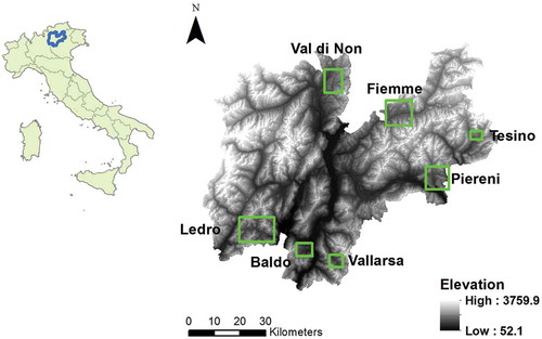
To analyze ES and biodiversity associated with agricultural areas in mountain landscapes with different land use intensity, we selected seven representative study sites in the Autonomous Province of Trento, an Alpine region in Northern Italy. A detailed analysis of the provision of multiple ES in this province is described in Ferrari and Geneletti (2014) and Ferrari et al. (2016), providing a background for this research. In particular, the selection of the study sites was carried out in collaboration with key staff from the provincial administration, responsible for the implementation of the agricultural policies in the province, among others. Figure 1 shows the distribution of the study sites, i.e. Val di Non, Baldo, Vallarsa, Ledro, Piereni, Fiemme, and Tesino. Overall, the sites are representative of the variety of mountain agricultural landscapes in the Province of Trento (see Table 1).

Table 1. General characteristics of the seven study sites. More details on the land use classes based on Level 3 CORINE 2006 reported in Table A1.

Name	Area (ha)	Avg. elevation (m a.s.l.)	Main crops
Val di Non	2248	903 m	Fruit trees with annual crops and meadows
Baldo	1478	633 mc	Mixed, i.e. vineyards fruit trees, meadows, and annual crops
Vallarsa	492	784 m	Annual crops and meadows
Ledro	1185	756 m	Hay meadows with some mixed crops
Piereni	372	1134 m	Pastures and annual crops
Fiemme	2532	1086 m	Hay meadows and annual crops
Tesino	1848	915 m	Annual crops and pastures with some mixed crops

Figure 1. Location of the Autonomous Province of Trento in Italy (left) and of the seven study sites within the Province (right).

Operationally, for each selected study site, we extracted the agricultural areas (i.e. code 2) as identified in a 2013 land cover map, which is based on an update of the CORINE 2006 by the Autonomous Province of Trento. Following, we gathered the related cadastral and economic data to be used in the successive analysis (from the statistics of the Autonomous Province of Trento, 2013). The main characteristics of the study areas in terms of extension, elevation, and main types of crops are presented in Table 1. More details on the land use classes based on Level 3 CORINE 2006 are reported in Table A1 in the Appendix.

2.2. Assessment of ecosystem services and biodiversity

In line with the multifunctionality concept, in our analysis, we focused on the two main categories of ES associated with agricultural areas, namely: provisioning and cultural services, as identified by the Common International Classification of ES (Haines-Young and Potschin 2013). For each category, with the help of key staff form the provincial administration, we identified those ES that are considered the most significant in the context of the Autonomous Province of Trento. Similarly, we included four biodiversity indicators representing the provision of habitat for key animal and plant species in the region. In the following, the indicators selected for each ES and biodiversity, as well as the methods applied for their spatially-explicit assessment are briefly described.

2.2.1. Provisioning services

Agricultural production of food (i.e. ‘cultivated crops’ according to the CICES v4.3) and the production of forage (i.e. ‘fibers and other materials from plants, algae and animals for direct use or processing) were selected as the two most representative provisioning services for comparing the seven study areas. For each of these services, an indicator was selected: the annual overall market value of foodstuffs (apples, small fruits, vegetables, etc.) and the annual total market value of the forage product, respectively. Both indicators are expressed in Euro per hectare.

More specifically, data on crop typology were obtained from the statistics of the Autonomous Province of Trento (Servizio Politiche Sviluppo Rurale, PAT, 2013). In this database, the distinction between crops is based on declarations made by the individual farmers, followed by sample verification by the administration. Average productivity per hectare for each type of crop and market values were derived from provincial statistics (ISPAT, Istituto di statistica della provincia di Trento) or from the market values periodically collected by farmer and trade organizations (full details in Ferrari and Geneletti 2014).

2.2.2. Cultural services

Services related to the use (i.e. ‘physical use of land-/seascapes in different environmental settings’ according to the CICES v4.3) and the perception (i.e. ‘experiential use of plants, animals and land-/seascapes in different environmental settings’) of agricultural areas were considered. Accordingly, the indicators described in Table 2 were selected, namely: density of geotagged photographs; density of elements of cultural/aesthetic interest; density of cycling paths, hiking trails, horse trails, and mountain biking trails; and hunting (hares and small avifauna). Noteworthy, in the analysis, we arguable added a buffer of 200 m to the extracted agricultural areas, to account for ‘boundary effects’ linked to the production of ES that may occur outside of the area, but could actually be attributed to the area itself.

Table 2. Indicators selected for the cultural services.

Indicator	Explanatory notes
Density of geotagged photographs.	This provides a proxy of the degree of fruition of the agricultural areas by people who appreciate its aesthetic and landscape value, as well as its recreational function. The method (adapted from Orsi and Geneletti 2013 and Tenerelli et al. 2017) involves the collection of the photographs available on the ‘Panoramio’ website, one of the main photo sharing sites with a geographic location system. Density maps of photographs were constructed by considering for each cell (20X20 m) a radius of 500 m and reporting the number of photographs present within.
Density of elements of cultural/aesthetic interest.	This expresses the aesthetic and cultural value of the territory, based on the distribution of the elements of particular importance. These elements, which include areas of high landscape and environmental value, local reserves, and archeological sites, were identified based on the information contained in the Spatial Plan of the Autonomous Province of Trento. ArcMap 10.1 (ESRI) ‘Focal Statistics’ module was used to calculate the number of cells (100 m x 100 m) with at least one element of interest within 500 m. Hence, the ratio in percentage between the number of cells with elements of interest and the total areal extension of the study area was calculated.
Density of cycling paths, hiking trails, horse trails, and mountain biking trails.	This provides a quantification of the potential of the territory to be enjoyed for recreational purposes on foot and by bicycle. Based on data on pedestrian and cyclist paths (obtained from the Autonomous Province of Trento) and on hiking trails (from the local Alpine Club), the density of these elements was calculated and expressed in km/km^2.
Annual hunting (hares and small avifauna).	Hunting may also be considered a provisioning service, but here we highlighted its recreational nature, rather than that related to nutrition requirements or the integration of income that may arise from the consumption or sale of hunted animals. The analysis was limited to hares and small avifauna because they are present in open spaces and agricultural lands. The data used for the calculation of the indicator were the maps of the hunting reserves and the related database containing information on the registered hunters (more details in Ferrari and Geneletti 2014). The indicator was expressed in kilograms of wild game per hectare.

2.2.3. Biodiversity

The aim here was to deepen aspects related to the role of agricultural areas in preserving and promoting biodiversity, building on some important modeling efforts carried out within a recent European project (LIFE11/NAT/IT000187 T.E.N – Trentino Ecological Network – http://www.lifeten.tn.it/?lang=2). As shown in detail in Table 3, four biodiversity related indicators were selected, namely: number of focal animal species; conservation value of priority focal species; number of endemic and sub endemic floristic species; and (total) floristic richness. Also here, we considered a buffer of 200 m to the extracted agricultural areas, to account for ‘boundary effects.’

An overview of the representative ES selected for comparing the study areas, classified according to the CICES, and their respective indicators is given in Table 4.

Table 3. Indicators selected for biodiversity conservation.

Indicator	Explanatory notes
Number of focal animal species.	Computed based on the maps of the habitats of 55 focal species (see Appendix Table A2). It corresponds to the total number of focal species whose potential habitat (with medium and high eligibility) falls into the analyzed grid cell. The potential habitat was mapped during the above-mentioned European LIFE project based on algorithm implemented in the Maxent software (Phillips et al. 2006).
Conservation value of priority focal species.	Estimated by adding the conservation value of all the priority species whose habitat falls into a given location. The conservation values were estimated according to specific importance, the ecological and functional role and the extinction risk, based on the results of the mentioned LIFE project (See Table A2).
Number of endemic and sub endemic floristic species and Floristic richness.	Derived from an existing map (1-km cell size) that shows the number of endemic and sub-endemic species. Here only cells that are included in the selected agricultural areas for at least 20% were considered. The average number of endemic and sub endemic species and the total number of species per study area was calculated from the chosen cell.

Table 4. Overview of the selected ES classified according to the CICES system and their respective indicators.

Section	ES (CICES V4.3)	Indicator	Unit
PROVISIONING SERVICES	Cultivated crops	P1. Annual overall market value of foodstuff	€/ha
	Fibers and other materials from plants, algae and animals for direct use or processing	P2. Annual total market value of the forage product	€/ha
CULTURAL SERVICES	Experiential use of plants, animals and land-/seascapes in different environmental settings	C1. Density of geotagged photographs	Number of photos/km^2
	Experiential use of plants, animals and land-/seascapes in different environmental settings	C2. Density of elements of cultural/aesthetic interest	%
	Physical use of land-/seascapes in different environmental settings	C3. Density of cycling paths, hiking trails, horse trails, and mountain biking trails	km/km^2
	Physical use of land-/seascapes in different environmental	C4. Annual hunting (hares and small avifauna)	kg/ha
BIODIVERSITY	–	B1. Number of focal animal species	Animal species/km^2
	–	B2. Conservation value of priority focal species	Animal sp. value/km^2
	–	B3. Number of endemic and sub endemic floristic species	End. plant species/km^2
	–	B4. (Total) Floristic richness	Total plant species/km^2

2.3. Analysis of tradeoffs and synergies among ES and biodiversity, and identification of hotspots

To enable the analysis of tradeoffs and synergies, as a first step, the values of the selected indicators values were normalized between 0 and 1, assigning 1 to the maximum value according to the formula:

(1) $n_{score}=\frac{score}{highestscore}$(1)

where $n_{score}$ is the normalized value; $score$ is the original value and $highestscore$ is the maximum value found for that indicator in the seven study areas considered.

The normalized indicators values of were thus used to jointly display the ES provision of the seven study areas. This was done using ‘flower’ diagrams (more commonly referred to as spider plots) in which the length of each axis is proportional to the maximum provision of the service in question (see Foley 2005). Furthermore, to gain a general understanding of the potential tradeoffs and synergies among ES and biodiversity, beyond the specific study areas, an explorative correlations analysis was carried out considering the 10 normalized indicators. The correlation analysis was performed using R software; specifically, the ‘car’ package (Fox and Weisberg 2011).

Following, to simplify the reading and interpretation of the analysis of tradeoffs and synergies, a two-step aggregation of the normalized indicators was undertaken. The first step consisted of calculating the arithmetic mean to obtain a single indicator for perception-related socio-cultural services (i.e. C1 and C2), and a single indicator for use-related socio-cultural services (i.e. C3 and C4), a single aggregated indicator for habitat support for fauna (i.e. B1 and B2), a single indicator for habitat support for flora (i.e. B3 and B4). The second-step consisted of aggregating the indicators into the two main categories of the CICES system, i.e. provisioning and cultural services, and biodiversity. As far as provisioning category was concerned, an additional aggregation step was performed in which, by way of example, the forage production was overlooked (given its values expressed in Euros per hectare were relatively much lower than the values obtained for food production). Flower diagrams were prepared, and correlation analysis performed with respect to the aggregated indicators.

As a final step, to identify spatial patterns of ‘hotspots’, i.e. areas characterized by high levels of provision of multiple services and biodiversity, the maps of the ES were superimposed. The rationale behind is that identifying hotspots can offer a reference for scientifically defining boundaries for specific agro-environmental and conservation measures (e.g. Zhang et al. 2015). More specifically, the individual ES maps were first normalized and later summed through GIS Map Algebra operations. While an extensive literature has developed on the identification of ‘hotspots’, here, the aim was to provide a first overview of the spatial distribution of the potential tradeoffs and synergies among ES and biodiversity as background for further analysis.

3. Results

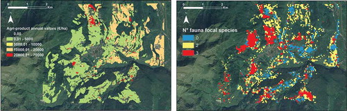
Figure 2 presents two illustrative maps of ES and biodiversity indicator for the Baldo study site. It shows the spatial distribution of the annual overall market value of foodstuff (P1) and number of fauna focal species (B1) within the agricultural area, classified as code 2 according to the Level 1 CORINE 2006. Similar maps of the spatial distribution of the 10 selected ES and biodiversity indicators were generated for all the seven study sites and, as described later, used for the hotspot analysis. The overall values of the 10 selected ES and biodiversity indicators are shown in Table A3 in the Appendix.

Figure 2. Illustrative maps of ES and biodiversity indicators for the Baldo study area: P1 – overall market value of foodstuff (left) and B1 – number of fauna focal species (right).

The normalized ES and biodiversity indicators (both individually and aggregated) were used for the analysis of tradeoffs and synergies presented in the next section, including flower diagrams and correlation analysis. The normalized values of the selected ES and biodiversity indicators are shown in Table A4 (10 individual indicators), in Table A5 (six aggregated indicators), and Table A6 (three aggregated indicators), in the appendix.

3.1. Results for individual ES and biodiversity indicators

The ‘flower’ diagrams in Figure 3 allow making a comparison of the study areas based on the selected 10 ES and biodiversity indicators. Noteworthy, the study sites are here ordered based the total value of the provisioning services (i.e. P1+ P2), here assumed to be a good proxy of agricultural land-use intensity. The values range from €/ha 10.790 for Val di Non to €/ha 1.958 for Tesino study area, against a national average value of €/ha 2.414 according to the Farm Accountancy Data Network (FADN).

Figure 3. Flower diagrams representing the normalized value of the 10 selected ES and biodiversity indicator for the seven study areas. Individually, each flower diagram allows visualizing the tradeoffs and synergies among ES and biodiversity within a study area; overall, the diagrams allow comparison of the performance of the study areas. Note that the study sites are displayed based on the actual values in €/ha of the indicators of the provisioning services (P1 + P2), representing a good proxy of agricultural land-use intensity. Accordingly, the study areas are divided into three groups of agricultural land-use intensity while also specifying the degree of ‘multifunctionality’, i.e. number of ES and biodiversity indicators exceeding the threshold value of 0.5 (see bottom).

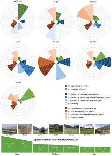
Accordingly, the flower diagrams illustrate how a broad range of ES characterizes some agricultural areas while others have peak values only for specific ES and/or biodiversity indicators. For example, the Val di Non (€/ha 10.790) and Tesino (€/ha 1.958) study areas appear to be the most markedly ‘mono-functional’ ones, i.e. providing only two out of the 10 selected ES (considering a threshold value of 0.5 to determine whether an area provides a given ES). In Val di Non, the maximization of agricultural productivity seems to take place at the expense of all other services, while the Tesino study site has the highest average production of forage. The Vallarsa (€/ha 3.707) study site has the highest values of biodiversity indicators, represented by the flora and the number of focal species. The Baldo (€/ha 6.111), Ledro (€/ha 3.058), and Fiemme (€/ha 2.375) sites have similar characteristics in terms of providing multiple services. All characterized by three high-value indicators belonging to two different categories, i.e. provisioning and cultural for Fiemme, and cultural services and biodiversity for Baldo and Ledro. The Piereni area shows some synergy between cultural services and biodiversity indicators against low values for the provisioning services.

Overall, considering a threshold value of 0.5, the study areas can be arguably divided into three groups based on their agricultural intensity, i.e. high (Val di Non and Baldo); medium (Vallarsa, Ledro, and Piereni) and low (Fiemme and Tesino), specifying their degree of multifunctionality (as shown in Figure 3).

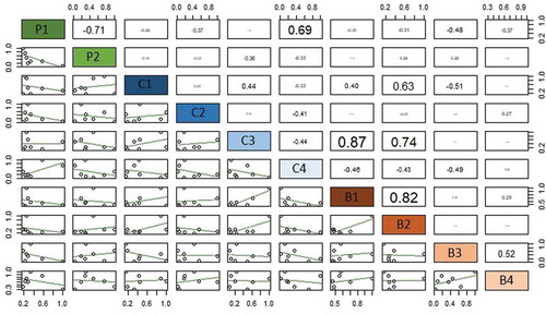
More general consideration, beyond the specific study sites, can be made based on the results of the correlation analyses among the selected 10 indicators (see Figure 4). For example, it is possible to argue that the most significant positive correlations are the ones between B1-Number of focal animal species and C3-Density of cycling and pedestrian paths (0.87), between B1-Number of focal animal species and B2-Value of priority focal species (0.82); between B2-Value of priority focal species and C3-Densify of cycling and pedestrian paths (0.74); and finally between P1- Agricultural production and C4- Hunting (0.69). Similarly, it is possible to state that the highest negative correlation are registered between P1-Agrucultural production and P2-Forage production (−0.71), and between B3 Endemic and sub endemic floristic species and C1 Density of geotagged photographs (−0.51).

Figure 4. Results of the correlation analysis among the 10 selected ES indicators represented using a so-called ‘Scatterplot matrix’. The matrix contains the correlation values between the indicators expressed in the range ± 1 (upper diagonal) and a graphical representation of the data (in the lower diagonal).

3.2. Results for aggregated ES indicators

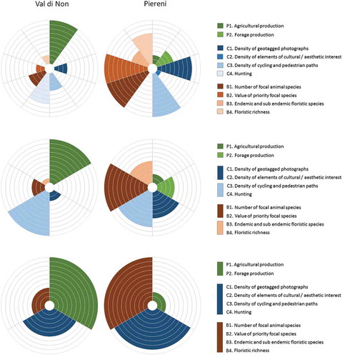
The results based on the aggregated indicators, including flower diagrams and related correlation analysis, are reported in the appendix: Figure A1 and Figure A2 (six aggregated indicators), Figure A3 and Figure A4 (three aggregated indicators), andFigure A5 and Figure A6 (three aggregated indicators, overlooking P2 – Forage production). Instead, the focus here is on some potential biases related to the aggregation of the indicators, originally aimed at simplifying the reading of the analysis of tradeoffs and synergies. Figure 5 is an example of how the two-step aggregation of the ES and biodiversity indicators can actually bias the interpretation of the results. More specifically, two illustrative study sites (i.e. Val di Non and Piereni) are compared based on the aggregated indicators. Noteworthy is how, with increasing level of aggregation of the indicators, some tradeoffs and synergies may actually go undetected, highlighting the importance of adopting the required level of disaggregation in order to correctly inform decisions.

Figure 5. Comparison of the two study areas with respect to individual and aggregated ES indicators. Note how the aggregation of the indicators may hide ES tradeoffs and synergies, ultimately, leading to different decisions.

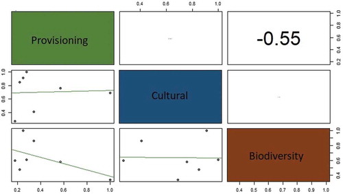
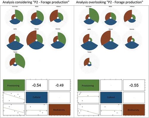
Another example of how the applied aggregation criteria can significantly change the results is shown Figure 6. In this case, the comparison is between an aggregation that considers both food and forage production (P1 and P2) and one that considers only food production (P1) overlooking the forage production (P2) whose maximum monetary values are relatively much lower (i.e. €/ha10790 against €/ha 27). The differences are particularly evident in the case of the Tesino study areas with respect to the provisioning services. Moreover, the different aggregation criteria result in different correlation values, which can lead to some important tradeoffs to be neglected (e.g. between provisioning and cultural services) or slightly underestimated (e.g. between provisioning services and biodiversity).

Figure 6. An example of how different aggregation criteria (including both F1 and F2 indictors or only F1) can affect the different results, leading to support different conclusions (e.g. overlooking negative correlation between regulating/maintenance and cultural services).

3.3 Identifications of hotspots

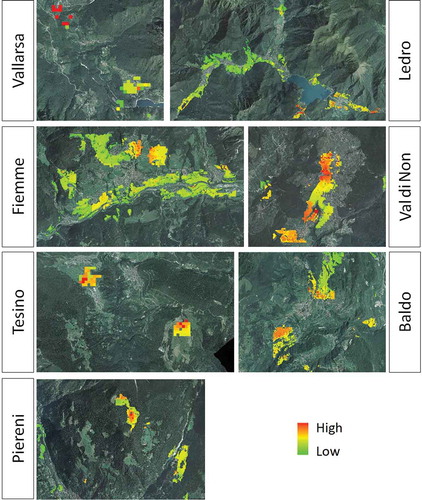
The spatial distributions of hotspots, which indicate the presence of multiple ES provided by the agricultural areas, are shown in Figure 7. The maps highlight that in some of the study areas the provision of ES is evenly distributed within the entire agricultural area. This is the case for example in the Fiemme and Baldo areas. In other cases, the supply is more scattered, with a sharp contrast between the hotspots and the remaining agricultural areas (see e.g. Tesino and Vallarsa).

Figure 7. Spatial distribution of hotspots, i.e. areas characterized by high level of ES provision and biodiversity, in the seven study agricultural areas.

4. Discussion

The comparison of the selected study areas highlighted differences in the range of the provided ES and the levels of biodiversity, and their respective tradeoffs and synergies. This is particularly useful to address key questions dealing with the interaction between ES provided by different agricultural areas (Lee and Lautenbach 2016). Overall, the findings confirm that a gradient from extensive to intensive forms of agricultural land use, in addition to the loss of habitats, also involves a reduction of services related to cultural, aesthetic and perception values. Other synergies mentioned in the literature were also verified (Howe et al. 2014): areas characterized by higher values of provision of food or forage, for example, showed lower values with respect to habitat provision for animal and plant species as well as to cultural services. Moreover, within the study sites, significant correlation could be identified among cultural services and biodiversity. Indeed, the correlation analysis was an effective way to synthesizing the results, allowing making general, and quantifiable considerations about the relationship between different indicators. Despite the limited number of our study sites, this type of analysis can help identify the most significant positive and negative correlations between indicators, which can be used to further investigate potential tradeoffs and synergies among multiple ES and biodiversity indicators (e.g. through dynamic modeling approaches).

The mapping of hotspots, i.e. areas characterized by the provision of high levels of ES and biodiversity, provides important references for landscape management and planning, but also supporting management actions that, aimed at seizing the differentiated opportunities across the landscape, may prioritize different services in different areas (Raudsepp-Hearne et al. 2010). Accordingly, it was here assumed that when multiple ES are identified across broad regions, any spatial overlap represents a particular type of ES interaction, which can be quantified using correlation coefficients: positively correlated ES being assumed to be synergistic whereas negatively correlated ES are presumed to be trade-offs (Raudsepp-Hearne et al. 2010; Tomscha and Gergel 2016). Nevertheless, several approaches exist to identify hotspots, which can be classified into two main typologies: a first one based on defining a certain threshold to determine hotspots and second one based on spatial aggregation/clustering analysis, such as the Kernel density estimation (Li et al. 2017). A critical weakness of the threshold or quantiles-based method is due to the fact that they may cause the landscape connectivity between or within the identified hotspots to be ignored, which can ultimately lead the ES assessment to support undesirable landscape fragmentation (e.g. Mitchell et al. 2015). Therefore, the mapping of ES hotspot in our study sites has to be interpreted rather cautiously and is to be considered a starting point for further analysis.

In line with an emerging interest in the literature (Cash et al. 2003; Clark et al. 2016), the proposed assessment of tradeoffs and synergies among ES and biodiversity associated with agricultural areas implicitly addresses issues related to the usefulness and usability of the generated results in an operational setting. To start with, we here propose the use multiple ES and biodiversity indicators that capture diverse stakeholders’ perspectives: a crucial step in disentangling the different contributions to ES by different typologies of agricultural land uses with respect to different types of beneficiaries (Martín-López et al. 2012). Particularly, the different ES in the study sites are potentially used by people from different places, which is a relevant issue to consider when planning for multi-functional agriculture (e.g. in the urban-rural interface). The assessment of the provisioning ES indicators, for example, relied on data collected routinely by the local administration by involving the farmers. In the case of cultural services, the use of geotagged photographs has been criticized for excluding a part of the population (i.e. elder population). In fact in mountain areas like Trento, it might be the case that a reduced amount of the population uses Panoramio and you could not differentiate different types of users (e.g. residents from tourists). These and others, are key elements to mainstreaming ES in decision-making (e.g. Geneletti 2013), and to use this kind of analysis as a monitoring tool to assess the effectiveness of policies supporting multifunctionality. To this purpose, efforts to summarize and better communicate the results (e.g. flower diagrams and correlation analysis) are essential, particularly in participatory stakeholders setting. These are all elements that collectively contribute to enhancing the potential usefulness and usability of the results, by ensuring their scientific credibility and their saliency (e.g. Adem Esmail and Geneletti 2017; Adem Esmail et al. 2017).

Concerning the adopted methodology, normalization and aggregation of indicators values were two critical steps of the assessment of tradeoffs and synergies among ES. Normalization consists in converting the ‘raw’ value of the ES indicators, expressed their respective units (e.g. €/h), into a dimensionless scale of preference, that is, a dimensionless expression of the level of desirability of the specific indicators as typically done in a multicriterion analysis (Geneletti 2005a, 2005b). Here, for example, the normalization was simply performed with respect to the maximum indicator values among the seven study areas. Nevertheless, several approaches exist to perform normalization, and some of these approached require inputs from relevant stakeholders that can be collected using specific techniques, such as value functions (for more on this refer to Adem Esmail & Geneletti 2018; Beinat 1997; Geneletti 2004). Therefore, it is important to discuss this aspect with the stakeholders and to test different normalization approaches. Similarly, aggregation of the selected indicators is also crucial step of the ES assessment enabling the analysis of tradeoffs and synergies. It refers to the application of a rule (e.g. an algebraic expression) to combine the values of more indicators. Different rules could be applied, from a simple arithmetic mean (as done for simplicity, in this paper) to weighted linear combination or other more complex rules. Therefore, to test the robustness of the results considering the uncertainty factors related to the different steps (of normalization and aggregation) it is important that future studies include a sensitivity analysis to explore the relationship between the output and the input of the process (see e.g. Saltelli et al. 2000).

Finally, considering the specific application reported in the paper, the limited number of study sites does not allow deriving models to generalize and improve the understanding of the direct and indirect causes for variations in ES. These constitutes the main limitations of the study, implying the impossibility to infer trade-offs and synergies between ES and biodiversity associated with the different arrangements of crops and land uses. Nonetheless, the indicators allowed producing relevant ES and biodiversity maps (e.g. Figure 2) that can be used as a starting point for further analyses (for example, using more detailed information from field surveys or interviews), and can provide useful guidance to support spatial and sectoral planning. Among others, the approach can be used to assess the effectiveness of policies and actions directed toward multifunctionality, by using our maps as the baseline reference against which to measure progresses toward a more multifunctional agricultural space.

5. Conclusions

In this study, we assessed the tradeoffs and synergies among the ES and biodiversity indicators associated with different mountainous agricultural landscapes. Through a quantitative and spatially explicit assessment of the tradeoffs and synergies among ES and biodiversity, the proposed approach can support key planning and management decisions that aim to promote multifunctionality of mountain agriculture. Specifically, we performed a quantitative and spatially explicit evaluation of 10 ES and biodiversity indicators for seven selected study sites that are representative of agricultural areas in mountain landscapes. Thus, the research contributed to the growing literature on the analysis of tradeoffs and synergies to inform policy-and decision-making (e.g. Geneletti 2013; Daw et al. 2015). Moreover, the concept of multifunctionality has been operationalized by analyzing the provision of a bundle of ES representing provisioning and cultural services together with a set of biodiversity indicators.

An important conclusion that emerged from the application of the proposed approach is the fact that tradeoffs and synergies among ES and biodiversity can be hidden or highlighted depending on how specific methodological steps are performed, such the normalization and the aggregation of the selected ES indicators. This is well illustrated by the flower diagrams based on different aggregation of indicators, which present significant differences in the results. For example, the polarization towards one or two categories of ES or a more balanced provision of ES may not appear equally clear when considering individual services. Nevertheless, individual services cannot be used to draw generalized results about a whole category. The assessment of tradeoffs and synergies between ES should consider multidimensional aspects of provision and, possibly, different spatial scales (or different level of aggregation) in the data.

Acknowledgements

This study received funding from the Autonomous Province of Trento (Servizio Sviluppo sostenibile e Aree protette). We would like to thank the Science Museum of Trento (MUSE, contact person: Dr. Paolo Pedrini) for making available the species distribution data, and the technical offices of the Autonomous Province of Trento for providing the data on land use and infrastructures. We are grateful to Prof. Angus Morrison-Saunders and Dr. Jenny Pope for helpful comments on early versions of this paper.

Disclosure statement

No potential conflict of interest was reported by the authors.

Appendix

Table A1. Land-use classes in the seven study sites, based on Level 3 CORINE 2006.

Land-use class	Val di Non	Baldo	Vallarsa	Ledro	Piereni	Fiemme	Tesino
Code	ha	ha	ha	ha	ha	ha	ha
211	–	–	–	–	–	–	138.1
221	–	61	–	–	–	–	–
222	734,4	–	108,1	–	–	–	–
231	1465,2	538,1	–	724,7	88,6	844,2	357,9
241	–	248,8	–	134,6	–	745,8	–
242	46.7	21,5	–	69,7	0,4	99,9	177,5
243	2.2	607,0	383,6	255,9	282,8	841,9	1174,0
Total	2248,4	1478,4	491,7	1184,9	371,8	2531,7	1847,5

211 – non-irrigated arable land; 221 – vineyards; 222 – fruit trees and berry plantations; 231 – lastures; 241 – annual crops associated with permanent crops; 242 – complex cultivation patterns; 243 – land principally occupied by agriculture, with significant areas of natural vegetation.

Table A2. List of the focal species considered in the index B1 – number of focal animal species. In bold, the priority focal species and their conservation value used in the index B2 – conservation value of priority focal species.

Accipiter gentilis	Crex crex (61,9)	Otus scops
Acrocephalus scirpaceous	Cyanistes caeruleus (ex Parus caeruleus)	Pernis apivorus (24,6)
Aegolius funereus (42,1)	Dendrocopos major	Phoenicurus phoenicurus
Alectoris graeca (72,2)	Dryocopus martius (43,7)	Picus canus (45,2)
Anas platyrhynchos	Emberiza citrinella	Picus viridis
Aquila chrysaetos (47,6)	Falco tinnunculus	Podiceps cristatus
Ardea cinerea	Fulica atra	Prunetta collaris
Bombina variegata (56,5)	Gallinula chloropus	Rallus acquaticus
Bonasa bonasia (42,1)	Glaucidium passerinum (50)	Salamandra salamandra
Bufo bufo	Gypaetus barbatus (54)	Saxicola rubetra
Buteo buteo	Jynx torquilla	Sitta europaea
Caprimulgus europaeus (50,8)	Lagopus muta (52,4)	Tachybaptus ruficollis
Carduelis cannabina	Lanius collurio (51,6)	Tetrao tetrix (43,7)
Carduelis cannabina	Lophophanes cristatus (ex Parus cristatus)	Tetrao urogallus (57,9)
Certhia brachydactyla	Marmota marmota	Turdus torquatus
Certhia familiaris	Milvus migrans (37,3)	Upupa epops
Cettia cetti	Montifringilla nivalis	Ursus arctos (70,4)
Cinclus cinclus	Oenanthe oenanthe	Zootoca vivipara
Coturnix coturnix

Table A3. Value of the 10 selected ES and biodiversity indicator for the study areas expressed in their respective units.

Indicator	Unit	Val di Non	Baldo	Vallarsa	Ledro	Piereni	Fiemme	Tesino	MAX
P1	€/ha	10,789,5	6103,3	3698,5	3052,3	2722,4	2354,7	1931,0	10,789,5
P2	€/ha	0,8	7,8	8,5	5,2	12,9	20,3	27,0	27,0
C1	Number of photos/km^2	6,65	8,80	3,26	9,12	18,06	20,28	3,56	20,28
C2	%	1,10	3,90	8,80	20,70	3,50	11,30	0,40	20,70
C3	km/km^2	0,89	0,19	0,42	1,13	1,83	0,38	0,13	1,83
C4	kg/ha	4,37	6,24	0,67	1,27	0,11	1,05	2,22	6,24
B1	Animal species/km^2	1,11	1,25	1,31	1,60	2,29	1,05	1,09	2,29
B2	Animal sp. value/km^2	11,21	10,84	7,19	11,21	41,40	15,53	15,47	41,40
B3	Endemic plant species/km^2	0,32	2,03	11,00	3,90	5,00	0,81	7,00	11,00
B4	Total plant species/km^2	77,50	224,10	265,50	161,00	195,10	168,00	110,90	265,50

Table A4. Normalized value of the 10 selected ES and biodiversity indicator for the seven study areas.

Indicator	Val di Non	Baldo	Vallarsa	Ledro	Piereni	Fiemme	Tesino
P1	1,00	0,57	0,34	0,28	0,25	0,22	0,18
P2	0,03	0,29	0,31	0,19	0,48	0,75	1,00
C1	0,33	0,43	0,16	0,45	0,89	1,00	0,18
C2	0,05	0,19	0,43	1,00	0,17	0,55	0,02
C3	0,49	0,11	0,23	0,62	1,00	0,21	0,07
C4	0,70	1,00	0,11	0,20	0,02	0,17	0,36
B1	0,48	0,55	0,57	0,70	1,00	0,46	0,48
B2	0,27	0,26	0,17	0,27	1,00	0,38	0,37
B3	0,03	0,18	1,00	0,35	0,45	0,07	0,64
B4	0,29	0,84	1,00	0,61	0,73	0,63	0,42

Table A5. Average normalized values of the ES and biodiversity indicators aggregated into six categories.

Indicator	Val di Non	Baldo	Vallarsa	Ledro	Piereni	Fiemme	Tesino
P1	1,00	0,57	0,34	0,28	0,25	0,22	0,18
P2	0,03	0,29	0,31	0,19	0,48	0,75	1,00
C1, C2	0,25	0,40	0,38	0,94	0,69	1,00	0,13
C3, C4	1,00	0,93	0,28	0,69	0,86	0,32	0,36
B1, B2	0,38	0,40	0,37	0,48	1,00	0,42	0,42
B3, B4	0,16	0,51	1,00	0,48	0,59	0,35	0,53

Table A6. Average normalized values of the ES and biodiversity indicators aggregated into three categories.

Indicator	Val di Non	Baldo	Vallarsa	Ledro	Piereni	Fiemme	Tesino
F1, F2	0,87	0,72	0,56	0,40	0,62	0,82	1,00
C1, C2, C3, C4	0,69	0,76	0,41	1,00	0,91	0,85	0,27
B1, B2, B3, B4	0,34	0,58	0,86	0,61	1,00	0,48	0,60

Figure A1. Flower diagrams representing the normalized value of the 6 aggregated ES and biodiversity indicator for the seven study areas. Individually, each flower diagram allows visualizing the tradeoffs and synergies among ES and biodiversity within a study area; overall, the diagrams allow comparison of the performance of the study areas. Note that the study sites are displayed based on their value of agricultural land-use intensity (i.e. P1 + P2 expressed in €/ha). Accordingly, the study areas are divided into three groups of agricultural land-use intensity, specifying the degree of multifunctionality, i.e. number of ES and biodiversity indicators that exceed the threshold value of 0.5 (see bottom).

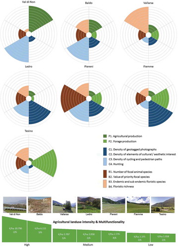
Figure A2. Results of the correlation analysis among the six aggregated ES and biodiversity indicators.

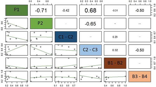
Figure A3. Flower diagrams representing the normalized value of the three aggregated ES and biodiversity indicator for the seven study areas, considering both food and forage production (P1 & P2). Singularly, each flower diagram allows visualizing the tradeoffs and synergies among ES and biodiversity within a study area; overall, the diagrams allow comparison of the performance of the study areas. Note that the study sites are displayed based on their value of agricultural land-use intensity (i.e. P1 + P2 expressed in €/ha). Accordingly, the study areas are divided into three groups of agricultural land-use intensity, specifying the degree of multifunctionality, i.e. number of ES and biodiversity indicators that exceed the threshold value of 0.5.

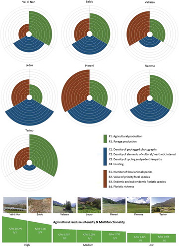
Figure A4. Results of the correlation analysis among the three aggregated indicators, considering both P1 Cultivated crops and P2 Forage production.

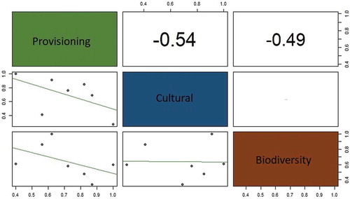
Figure A5. Flower diagrams representing the normalized value of the three aggregated ES and biodiversity indicator for the seven study areas, overlooking forage production (P2). Singularly, each flower diagram allows visualizing the tradeoffs and synergies among ES and biodiversity within a study area; overall, the diagrams allow comparison of the performance of the study areas. Note that the study sites are displayed based on their value of agricultural land-use intensity (i.e. P1 + P2 expressed in €/ha). Accordingly, the study areas are divided into three groups of agricultural land-use intensity, specifying the degree of multifunctionality, i.e. number of ES and biodiversity indicators that exceed the threshold value of 0.5.

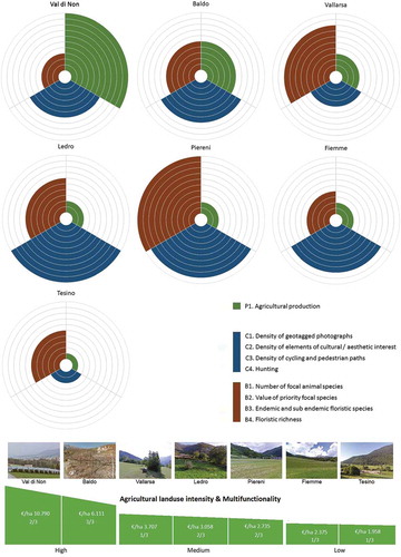
Figure A6. Results of the correlation analysis among the three aggregated indicators, considering only P1 Cultivated crops and overlooking P2 Forage production.

References

- Adem Esmail B, Geneletti D. 2017. Design and impact assessment of watershed investments: an approach based on ecosystem services and boundary work. Environ Impact Assess Rev [Internet]. 62:1–13. Available from http://linkinghub.elsevier.com/retrieve/pii/S0195925516300427.
- Adem Esmail B, Geneletti D. 2018. Multi-criteria decision analysis for nature conservation: a review of 20 years of applications. Methods Ecol Evol. 9:42–53.
- Adem Esmail B, Geneletti D, Albert C. 2017. Boundary work for implementing adaptive management: a water sector application. Sci Total Environ [Internet]. 593:274–285. Available from http://linkinghub.elsevier.com/retrieve/pii/S0048969717306332.
- Barton DN, Kelemen E, Dick J, Martin-Lopez B, Gómez-Baggethun E, Jacobs S, Hendriks CMA, Termansen M, García-Llorente MPrimmer E, et al. 2018. (Dis) integrated valuation – Assessing the information gaps in ecosystem service appraisals for governance support. Ecosyst Serv. 29:529–541.
- Baylis K, Peplow S, Rausser G, Simon L. 2008. Agri-environmental policies in the EU and United States: a comparison. Ecol Econ. 65:753–764.
- Beinat E. 1997. Value functions for environmental management [Internet]. Dordrecht: Springer Netherlands. Available from http://link.springer.com/10.1007/978-94-015-8885-0.
- Bennett EM, Cramer W, Begossi A, Cundill G, Díaz S, Egoh BN, Geijzendorffer IR, Krug CB, Lavorel S, Lazos E, et al. 2015. Linking biodiversity, ecosystem services, and human well-being: three challenges for designing research for sustainability. Curr Opin Environ Sustain [Internet]. 14:76–85. Available from http://linkinghub.elsevier.com/retrieve/pii/S1877343515000366.
- Braat L, Ten Brink P, editors. 2008. The cost of policy inaction: the case of not meeting the 2010 biodiversity target. Wageningen: Study for the European Commission, DG Environment. Alterra report 1718.
- Burkhard B, Kroll F, Müller F. 2010. Landscapes‘ capacities to provide ecosystem services – a concept for land-cover based assessments. Landsc Online [Internet]. 15:1–22. Available from http://www.landscapeonline.de/103097lo200915/.
- Cahill C. 2001. The multifunctionality of agriculture. EuroChoices [Internet]. 1:36–41. Available from. doi:10.1111/j.1746-692X.2001.tb00073.x.
- Cash DW, Clark WC, Alcock F, Dickson NM, Eckley N, Guston DH, Jager J, Mitchell RB. 2003. Knowledge systems for sustainable development. Proc Natl Acad Sci [Internet]. 100:8086–8091. Available from http://www.pnas.org/cgi/doi/10.1073/pnas.1231332100.
- Clark WC, Tomich TP, van Noordwijk M, Guston D, Catacutan D, Dickson NM, McNie E. 2016. Boundary work for sustainable development: natural resource management at the consultative group on international agricultural research (CGIAR). Proc Natl Acad Sci [Internet]. 113:4615–4622. Available from http://www.pnas.org/cgi/doi/10.1073/pnas.0900231108.
- Cortinovis C, Geneletti D. 2018. Mapping and assessing ecosystem services to support urban planning: a case study on brownfield regeneration in Trento, Italy. One Ecosyst [Internet]. 3:e25477. Available from https://oneecosystem.pensoft.net/articles.php?id=25477.
- Crossman ND, Bryan BA. 2009. Identifying cost-effective hotspots for restoring natural capital and enhancing landscape multifunctionality. Ecol Econ [Internet]. 68:654–668. Available from. doi:10.1016/j.ecolecon.2008.05.003.
- Daw TM, Coulthard S, Cheung WWL, Brown K, Abunge C, Galafassi D, Peterson GD, McClanahan TR, Omukoto JO, Munyi L. 2015. Evaluating taboo trade-offs in ecosystems services and human well-being. Proc Natl Acad Sci [Internet]. 201414900. Available from http://www.pnas.org/lookup/doi/10.1073/pnas.1414900112.
- de Groot RS, Alkemade R, Braat L, Hein L, Willemen L. 2010. Challenges in integrating the concept of ecosystem services and values in landscape planning, management and decision making. Ecol Complex [Internet]. cited 2013 Jul 31. 7:260–272. Available from doi:10.1016/j.ecocom.2009.10.006.
- Ekroos J, Olsson O, Rundlöf M, Wätzold F, Smith HG. 2014. Optimizing agri-environment schemes for biodiversity, ecosystem services or both? Biol Conserv [Internet]. 172:65–71. Available from http://linkinghub.elsevier.com/retrieve/pii/S0006320714000718.
- European Court of Auditors. 2011. Is agri-environment support well designed and managed? Luxembourg: Publications Office of the European Union. Special Report No 7.
- Ferrari M, Geneletti D. 2014. Mapping and assessing multiple ecosystem services in an alpine region: a Study in Trentino, Italy. Ann di Bot [Internet]. 4:65–71. Available from http://statusquaestionis.uniroma1.it/index.php/Annalidibotanica/article/view/11729.
- Ferrari M, Geneletti D, Cayuela L, Orsi F, Benayas JMR. 2016. Analysis of Bundles and Drivers of Change of Multiple Ecosystem Services in an Alpine Region. J Environ Assess Policy Manag [Internet]. 18: 1650026. Available from: http://www.worldscientific.com/doi/abs/10.1142/S1464333216500265
- Fichino BS, Pivello VR, Santos RF. 2017. Trade-offs among ecosystem services under different pinion harvesting intensities in Brazilian Araucaria Forests. Int J Biodivers Sci Ecosyst Serv Manag [Internet]. 13:139–149. Available from https://www.tandfonline.com/doi/full/10.1080/21513732.2016.1275811.
- Foley JA. 2005. Global consequences of land use. Science (80-) [Internet]. 309:570–574. Available from http://www.sciencemag.org/cgi/doi/10.1126/science.1111772.
- Fox J, Weisberg S. 2011. An R companion to applied regression. second. place unknown: Sage. editor.
- Geneletti D. 2004. A GIS-based decision support system to identify nature conservation priorities in an alpine valley. Land Use Policy. 21:149–160.
- Geneletti D. 2005a. Multicriteria analysis to compare the impact of alternative road corridors: a case study in northern Italy. Impact Assess Proj Apprais [Internet]. 23:135–146. Available from http://www.tandfonline.com/doi/abs/10.3152/147154605781765661.
- Geneletti D. 2005b. Formalising expert opinion through multi-attribute value functions: an application in landscape ecology. J Environ Manage [Internet]. 76:255–262. Available from http://linkinghub.elsevier.com/retrieve/pii/S0301479705001015.
- Geneletti D. 2011. Reasons and options for integrating ecosystem services in strategic environmental assessment of spatial planning. Int J Biodivers Sci Ecosyst Serv Manag [Internet]. 7:: 143–149. Available from http://www.tandfonline.com/doi/abs/10.1080/21513732.2011.617711.
- Geneletti D. 2012. Environmental assessment of spatial plan policies through land use scenarios. A study in a fast-developing town in rural Mozambique. Environ Impact Assess Rev [Internet]. cited 2013 Nov 7. 32:1–10. Available from http://linkinghub.elsevier.com/retrieve/pii/S019592551100028X.
- Geneletti D. 2013. Assessing the impact of alternative land-use zoning policies on future ecosystem services. Environ Impact Assess Rev [Internet]. cited 2013 May 24. 40:25–35. Available from http://linkinghub.elsevier.com/retrieve/pii/S0195925512001035.
- Geneletti D, Adem Esmail B, Cortinovis C. 2018. Identifying representative case studies for ecosystem services mapping and assessment across Europe. One Ecosyst [Internet]. 3:e25382. Available from https://oneecosystem.pensoft.net/articles.php?id=25382.
- Haines-Young R, Potschin M, editors. 2013. CICES V4.3-report prepared following Consultation 440 on CICES Version 4, August–December 2012. EEA Framework contract no. 441 EEA/IEA/09/003.
- Holland RA, Eigenbrod F, Armsworth PR, Anderson BJ, Thomas CD, Gaston KJ. 2011. The influence of temporal variation on relationships between ecosystem services. Biodivers Conserv [Internet]. 20:3285–3294. Available from http://link.springer.com/10.1007/s10531-011-0113-1.
- Howe C, Suich H, Vira B, Mace GM. 2014. Creating win-wins from trade-offs? Ecosystem services for human well-being: a meta-analysis of ecosystem service trade-offs and synergies in the real world. Glob Environ Chang [Internet]. 28:263–275. Available from http://linkinghub.elsevier.com/retrieve/pii/S0959378014001320.
- Kates BRW, Parris TM, Leiserowitz AA. 2005. What is sustainable development? Goals, indicators, and practice. Environment [Internet]. 47:8–21. Available from http://www.csa.com/partners/viewrecord.php?requester=gs&collection=ENV&recid=6248252.
- Kates RW. 2011. What kind of a science is sustainability science? Proc Natl Acad Sci. 108:19449–19450.
- Klapwijk C, van Wijk M, Rosenstock T, van Asten P, Thornton P, Giller K. 2014. Analysis of trade-offs in agricultural systems: current status and way forward. Curr Opin Environ Sustain [Internet]. 6:110–115. Available from http://www.sciencedirect.com/science/article/pii/S1877343513001607.
- Lastra-Bravo XB, Hubbard C, Garrod G, Tolón-Becerra A. 2015. What drives farmers’ participation in EU agri-environmental schemes?: Results from a qualitative meta-analysis. Environ Sci Policy [Internet]. 54:1–9. Available from http://linkinghub.elsevier.com/retrieve/pii/S1462901115300058.
- Lee H, Lautenbach S. 2016. A quantitative review of relationships between ecosystem services. Ecol Indic [Internet]. 66:340–351. Available from. doi:10.1016/j.ecolind.2016.02.004.
- Leventon J, Schaal T, Velten S, Dänhardt J, Fischer J, Abson DJ, Newig J. 2017. Collaboration or fragmentation? Biodiversity management through the common agricultural policy. Land Use Policy [Internet]. 64:1–12. Available from. doi:10.1016/j.landusepol.2017.02.009.
- Li Y, Zhang L, Yan J, Wang P, Hu N, Cheng W, Fu B. 2017. Mapping the hotspots and coldspots of ecosystem services in conservation priority setting. J Geogr Sci. 27:681–696.
- Locatelli B, Lavorel S, Sloan S, Tappeiner U, Geneletti D. 2017. Characteristic trajectories of ecosystem services in mountains. Front Ecol Environ [Internet]. 15:150–159. Available from. doi:10.1002/fee.1470.
- Martín-López B, Iniesta-Arandia I, García-Llorente M, Palomo I, Casado-Arzuaga I, Del ADG, Gómez-Baggethun E, Oteros-Rozas E, Palacios-Agundez I, Willaarts B, et al. 2012. Uncovering ecosystem service bundles through social preferences. Bawa K, editor. PLoS One [Internet]. 7:e38970. Available from. http://dx.plos.org/10.1371/journal.pone.0038970.
- Mastrangelo ME, Weyland F, Villarino SH, Barral MP, Nahuelhual L, Laterra P. 2014. Concepts and methods for landscape multifunctionality and a unifying framework based on ecosystem services. Landsc Ecol [Internet]. 29:345–358. Available from http://link.springer.com/10.1007/s10980-013-9959-9.
- McCracken ME, Woodcock BA, Lobley M, Pywell RF, Saratsi E, Swetnam RD, Mortimer SR, Harris SJ, Winter M, Hinsley S, et al. 2015. Social and ecological drivers of success in agri-environment schemes: the roles of farmers and environmental context. Finn J, editor. J Appl Ecol [Internet]. 52:696–705. Available from. doi:10.1111/1365-2664.12412.
- Mckenzie E, Posner S, Tillmann P, Bernhardt JR, Howard K, Rosenthal A. 2014. Understanding the use of ecosystem service knowledge in decision making: lessons from international experiences of spatial planning. Environ Plan C Gov Policy. 32:320–340.
- Mitchell MGE, Suarez-Castro AF, Martinez-Harms M, Maron M, McAlpine C, Gaston KJ, Johansen K, Rhodes JR. 2015. Reframing landscape fragmentation’s effects on ecosystem services. Trends Ecol Evol. 30:190–198.
- Moon W. 2015. Conceptualising multifunctional agriculture from a global perspective: implications for governing agricultural trade in the post-doha round era. Land Use Policy [Internet]. 49:252–263. Available from. doi:10.1016/j.landusepol.2015.07.026.
- OECD. 2003. Multifunctionality: the policy implications [Internet]. Paris (France): OECD Publishing. Available from http://www.oecd.org/tad/agricultural-policies/40782915.pdf.
- OECD. 2010. Linkages between agricultural policies and environmental effects [Internet]. Paris (France): OECD Publishing. Available from http://www.oecd-ilibrary.org/agriculture-and-food/linkages-between-agricultural-policies-and-environmental-effects_9789264095700-en.
- Orsi F, Geneletti D. 2013. Using geotagged photographs and GIS analysis to estimate visitor flows in natural areas. J Nat Conserv [Internet]. 21:359–368. Available from. doi:10.1016/j.jnc.2013.03.001.
- Phillips SJ, Anderson RP, Schapire RE. 2006. Maximum entropy modeling of species geographic distributions. Ecol Modell [Internet]. cited 2013 May 22. 190:231–259. Available from http://linkinghub.elsevier.com/retrieve/pii/S030438000500267X.
- Posner SM, McKenzie E, Ricketts TH. 2016. Policy impacts of ecosystem services knowledge. Proc Natl Acad Sci [Internet]. 113:201502452. Available from http://www.pnas.org/content/113/7/1760.short.
- Raudsepp-Hearne C, Peterson GD, Bennett EM. 2010. Ecosystem service bundles for analyzing tradeoffs in diverse landscapes. Proc Natl Acad Sci [Internet]. 107:: 5242–5247. Available from http://www.pnas.org/cgi/doi/10.1073/pnas.0907284107.
- Ruckelshaus M, McKenzie E, Tallis H, Guerry A, Daily GC, Kareiva P, Polasky S, Ricketts T, Bhagabati N, Wood SA, et al. 2015. Notes from the field: lessons learned from using ecosystem service approaches to inform real-world decisions. Ecol Econ [Internet]. 115:11–21. Available from http://linkinghub.elsevier.com/retrieve/pii/S0921800913002498.
- Saltelli A, Chan K, Scott EM. 2000. Sensitivity Analysis, Wiley series in probability and statistics. 1st ed. New York: John Wiley & Sons.
- Schneiders A, Van Daele T, Van Landuyt W, Van Reeth W. 2012. Biodiversity and ecosystem services: complementary approaches for ecosystem management? Ecol Indic [Internet]. 21:123–133. Available from. doi:10.1016/j.ecolind.2011.06.021.
- Seppelt R, Dormann CF, Eppink FV, Lautenbach S, Schmidt S. 2011. A quantitative review of ecosystem service studies: approaches, shortcomings and the road ahead. J Appl Ecol [Internet]. cited 2013 May 22. 48:630–636. Available from doi:10.1111/j.1365-2664.2010.01952.x.
- Tenerelli P, Püffel C, Luque S. 2017. Spatial assessment of aesthetic services in a complex mountain region: combining visual landscape properties with crowdsourced geographic information. Landsc Ecol. 32:1097–1115.
- Tomscha SA, Gergel SE. 2016. Ecosystem service trade-offs and synergies misunderstood without landscape history. Ecol Soc [Internet]. 21:art43. Available from http://www.ecologyandsociety.org/vol21/iss1/art43/.
- Van Huylenbroeck G, Vandermeulen V, Mettepenningen E, Verspecht A. 2007. Multifunctionality of agriculture: a review of definitions, evidence and instruments. Living Rev Landsc Res [Internet]. 1:1–43. Available from http://lrlr.landscapeonline.de/Articles/lrlr-2007-3.
- von Haaren C, Albert C. 2011. Integrating ecosystem services and environmental planning: limitations and synergies. Int J Biodivers Sci Ecosyst Serv Manag [Internet]. 7:150–167. Available from http://www.tandfonline.com/doi/abs/10.1080/21513732.2011.616534.
- von Haaren C, Galler C, Ott S. 2008. Landscape planning: the basis of sustainable landscape development [Internet]. place unknown: Bundesamt für Naturschutz/Federal Agency for Nature Conservation. Available from http://www.intechopen.com/books/landscape-planning.
- Willemen L, Veldkamp A, Verburg PH, Hein L, Leemans R. 2012. A multi-scale modelling approach for analysing landscape service dynamics. J Environ Manage [Internet]. 100:86–95. Available from. doi:10.1016/j.jenvman.2012.01.022.
- Zhang L, Fu B, Lü Y, Zeng Y. 2015. Balancing multiple ecosystem services in conservation priority setting. Landsc Ecol [Internet]. 30:535–546. Available from http://link.springer.com/10.1007/s10980-014-0106-z.