Causal inference in regression: advice to authors

The 2021 Nobel prize in economics was awarded to David Card, Joshua Angrist, and Guido Imbens. Card, together with his PhD supervisor the late Alan Krueger, developed empirical methods for investigating how policy interventions affect labor markets. Angrist and Imbens developed methods for identifying causes from real-world complexity. Collectively, this work on causal inference has come to redefine how economists conduct research. A parallel storey for the emergence and growth of causal methods unfolded a quarter-century earlier in the discipline of epidemiology (Hill, 1965). Formal methods for causal inference trace an even longer history, beginning with the work of Sewall Wright on biological development and inheritance (Wright, 1921, 1923, 1934).

Most empirical research published in Religion, Brain & Behavior is produced by scientists working in psychology, a field in which methods for causal inference remain poorly developed (see Rohrer, 2018). Here, we offer advice to RBB authors hoping to address causal inference using regression, ANOVA, and structural equation modeling.

Omitted variable bias

Researchers interested in causal identification must consider four types of causal confounding¹.

The first type of causal confounding is omitted variable bias. Suppose that we are interested in estimating the causal effect of an exposure X on an outcome Y. Omitted variable bias occurs when there is a common cause of both X and Y. Call this common cause Z. Figure 1(a) presents a graph of omitted variable bias: X ← Z → Y.

Figure 1. Suppose we are interested in estimating the causal effect of X (exposure) on Y (outcome). In each graph, the edges/arrows indicate directions of causal influence. Panels (a) and (b) present the same causal relationships: X does not influence Y, however, a third variable, Z, is a common cause both of X and Y. Panel (a) and (b) present two modelling choices: (a) Do not adjust for Z. This choice is indicated by the convention of a circular shape of the Z node. If our model were to omit to adjust for Z then X and Y would remain associated; however, this association would identify the causal effect of X on Y. Panel (b) presents a model that adjusts for Z. This is indicated by the convention of a square shape on the Z node. If our model were to adjust for Z, then the association between X and Y would be broken. Generalizing, to estimate the causal effect of an exposure on an outcome a statistical model of associations between variables needs to “close all back door paths” that may give rise to a non-causal association between the exposure and outcome. As we shall see, “closing all back door paths” between an exposure and outcome is necessary but not sufficient for causal inference. The remaining graphs follow the convention of a circular shape for an unadjusted covariate and a square shape for an adjusted covariate.

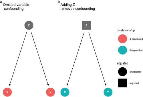
Here, X and Y are correlated because Z causes both. The association that Z induces gives an illusion of causality.

To see this, we can raise the following counterfactual: if we were to change X would there be a corresponding change in Y? The answer is no. When we include Z, the correlation between X and Y is broken (Figure 1(b)). All of the variation in X that predicts variation in Y is accounted for by variation in Z. In the language of causal inference, X is “conditionally independent” of Y given Z. The way to handle omitted variable bias is to adjust for Z in our statistical model. Generally, omitted variable bias requires closing all backdoor paths linking X and Y. We recommend that researchers include any variable that might induce a spurious association between an exposure and an outcome.

Post-treatment bias

The second type of confounding is “post-treatment” bias or “pipe confounding.” Suppose that we are interested in estimating the causal effect of an exposure X on an outcome Y. However, this time imagine a scenario in which Z is caused by X, and in turn, Y is caused by Z: thus X→ Z→ Y. In the language that is familiar to psychological scientists, we can say that Z “fully mediates” the relationship between X and Y.

Figure 2(a) graphically presents the scenario: X→ Z →Y. In this scenario, X causes Y: if we were to change X we would induce a change in Y. Although there is a causal effect of X on Y, if we were to include Z in our regression model we would break this relationship (Figure 2(b)). This is because all the variation that X causes in Y is contained in Z. Here, X and Y are conditionally independent given Z. Adding Z induces confounding because our interest is in the total effect of X on Y. If we were interested in the total effect of X on Y we should not include Z as a mediator in our statistical model.

Figure 2. (a) Z fully mediates the relationship between X and Y. In this scenario, taken in isolation, X and Y are correlated. (b) If we were to include Z in our model, X would be conditionally independent of Y. Adding Z confounds causal inference because we are interested in the causal effect of X on Y. Therefore, to obtain an unbiased causal estimate for the effect of X on Y, we should not include Z in our statistical model.

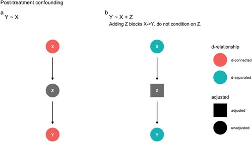
Psychological scientists are trained to control for as many variables that might affect X or Y. Post-treatment bias illustrates one of the perils in causal inference of “controlling for” the wrong variables. We recommend that researchers do not adjust for any mediator variable that could block a causal connection between an exposure and an outcome.

Our astute readers will have noticed that for omitted variable bias, the conditional independence of X on Y given Z is desirable, yet for post-treatment bias the conditional independence of X on Y given Z is undesirable. Our inferential strategy entirely turns on whether we draw a line from X→ Z ←Y (Z as an omitted variable) or X→ Z → Y (Z as a post-treatment mediator). How do we know whether Z is an omitted variable or a post-treatment variable? The data alone will not tell us whether Z is an omitted variable or whether Z is a treatment effect. Put simply, the data do not contain the causal assumptions needed for causal inference. Needed is a justification for choosing a causal model that is motivated by previous science and experience.

Collider bias

The third type of confounding is called collider bias. Imagine a scenario in which both X and Y cause Z yet X and Y are unrelated. As indicated in Figure 3(a), because X and Y are unrelated, the regression coefficient of X on Y will be unreliable. However, as indicated in Figure 3(b), if we were to include Z in our regression model we would open a path between X and Y giving an illusion of causation. Here, Z induces collider confounding. As indicated in Figure 3(c), to avoid bias we must omit Z from our regression model. In real life, the problem is more complicated. For example, bias in our sampling strategy may unintentionally cause us to stratify on a collider, biasing our estimates of X on Y. Likewise, missing data may introduce collider bias. There are methods for handling such biases (for example see: Barrett, 2021; McElreath, 2020; VanderWeele, 2015). However, sometimes the best researchers can do is estimate the sensitivity of their results to unavoidable confounding (VanderWeele et al., 2020).

Figure 3. (a) X and Y are unrelated. (b) By including Z in our model, X and Y become related. This is because knowing something about X will tell us something about Y. However, there is no causal relationship between X and Y. (c) The solution is to exclude collider confounders in our regression model. (d) Collider confounders are not restricted to observational data; they may arise in experimental data: here we see a plausible set of causal relationships between “control” variables in a multi-national experimental study. By restricting an adjustment set to the minimum required to close all back door paths, causal inference is possible: in a plausible causal model for this experiment, there is one minimal adjustment set available for inferring the theorized causal effect modification of the exposure (source) on the outcome (credibility) among people who vary by religiosity.

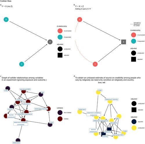
Experimental designs are useful for causal inference, yet experimental designs also risk confounding bias, such as collider confounding. Figure 3(d) presents indicators for variables that were collected as part of a multi-country experiment investigating the comparative credibility of scientists and religious elites (Hoogeveen et al., 2021). The study predicted there would be a causal effect modification of an exposure (source) on an outcome (credibility) among people who vary in religiosity. The crimson nodes identify potential collider confounders (ignoring the exposure and outcome). Indiscriminate inclusion of “control variables” in one's regression analysis risks introducing collider confounding - giving the illusion of an open causal path between the exposure variable and the outcome. How can we navigate the need to close all backdoor paths while avoiding collider confounding? As indicated in Figure 3(e), free and open-source software may be used to obtain the “adjustment sets” required to close back door paths with inducing collider or post-treatment confounding. In a plausible causal model for the relationships between variables in this experiment, the ggdag algorithm finds one minimal adjustment set for which there may be an unbiased estimate of the theorized causal effect modification {country, religiosity} (Barrett, 2021).² Note again that a causal model is assumed not verified. Causal inference occurs in a setting of intuitions informed by previous science (Wright, 1923).

Collider bias presents another instance of where “controlling for” too many variables introduces bias in causal estimation. Here, as in our discussion of post-stratification confounding, we place “controlling for” in scare quotes. We have seen that including variables without attending to confounding leads to bias in causal inference. Richard McElreath describes the habit of arbitrarily adding covariates as the “causal salad” approach:

But the approach which dominates in many parts of biology and the social sciences is instead CAUSAL SALAD. Causal salad means tossing various “control” variables into a statistical model, observing changes in estimates, and then telling a story about causation. Causal salad seems founded on the notion that only omitted variables can mislead us about causation. But included variables can just as easily confound us. When tossing a causal salad, a model that makes good predictions may still mislead about causation. If we use the model to plan an intervention, it will get everything wrong (McElreath, 2020, p. 46).

Because the world is complex, collider confounders may be hard to identify. We recommend that researchers use directed acyclic graphs (DAGs) to systematically identify and avoid collider (and other) forms of confounding (McElreath, 2020; Pearl, 2009; Pearl, 2019).

Descendent bias

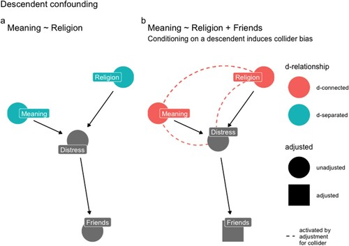
The fourth type of confounding may be called descendent bias. Descendent bias is a variation of post-treatment and collider bias. To condition on a variable that is caused by a parent variable is to partly condition on the parent. If the parent is a post-treatment confounder or a collider confounder, such conditioning will introduce bias. Figure 4 works through an example. Imagine we are interested in estimating the causal effect of Religion (exposure) on perceived Meaning (outcome). Suppose that both Religion and Meaning causally affect Distress (Figure 4(a)). Also, suppose that Distress causally affects one’s satisfaction with friendships (Friends) (Figure 4(a)). In this situation, “controlling for” one’s Friends would open a path between Religion and Meaning, biasing inference (Figure 4(b)). The solution here is to avoid conditioning on the descendent of a confounder: do not adjust for Friends (or Distress).

Figure 4. (a) X (Religion) and Y (Meaning) are unrelated. (b) If we were to “control for” a Friends (descendent) of Distress (collider) in our model, Religion (Exposure) and Meaning (Outcome) would appear to be related. The solution is to resist the impulse to include the descendent of a collider in a regression model.

Ten suggestions for causal inference

Researchers in the bio-cultural study of religion often use regression, ANOVA, and structural equation models to draw causal inferences from their data. Inferring causal effects lies at the heart of many scientific interests, yet we have noticed that without attention to causal confounding, statistical models can mislead. We offer the following guidance to authors for estimating causal effects while avoiding causal confounding.

1. We encourage researchers to consider that when they are interested in causal inference, they are interested in a counterfactual: how would a parameter in the world (Y) change if another parameter (X) were to change? As a first step in causal inference we suggest that RBB authors clarify the exposure variable(s) and the outcome variable(s) of interest to their study.

2. Authors who are interested in partitioning the total effect of X on Y into the direct effect of X on Y and the indirect effect of X on Y through Z should provide an explicit motivation for a mediation model as well as a strategy for casual identification (VanderWeele, 2015; VanderWeele, 2015). Without such care, authors risk using mediation in a manner that may induce post-treatment confounding.

3. We suggest that authors interested in causal inference submit a Directed Acyclic Graph (DAG) that clarifies all paths linking an exposure variable to an outcome variable, including unmeasured variables for which data have not been collected (McElreath, 2020). We suggest that authors also use their DAG(s) to identify omitted variable confounders, post-treatment confounders, collider confounders, and descendent confounders. Because causal identification may be complicated, we suggest that RBB authors avail themselves of software such as www.daggity.net (Textor et al., 2016) or the ggdag package in R (Barrett, 2021).

4. Causal inference requires closing all backdoor paths linking an exposure to an outcome. We recommend that researchers include any variable that might induce a spurious connection between the exposure and outcome of interest. Researchers should be aware that in some cases, closing backdoor paths will require more complicated approaches than we have had scope to cover here, such as obtaining instrumental variables (McElreath, 2020; VanderWeele, 2015).

5. Researchers should be aware that their DAG(s) are under-determined by their data. Where there is uncertainty about possible causal relationships, we recommend that authors present multiple DAGs. Authors should model results for each of the possible DAGs and clarify if and how inference changes as a result of assuming one graph over the others. Authors should feel no hesitation about reporting instances where bias in causal inference is unavoidable. Such a discovery may be important. Authors may also consider using a sensitivity analysis to assess the robustness of their inference to confounder biases (VanderWeele et al., 2020).

6. Where missing data are random conditional on other predictors in the model, we recommend that authors use a strategy for estimation that integrates over the uncertainty induced by missing data, such as regression using multiply imputed datasets or Bayesian imputation (McElreath, 2020).

7. Authors should limit “control variables” to the subset required to close backdoor paths (i.e. to handle omitted variable bias). Authors should not control for collider confounders or post-treatment confounders.

8. Authors should not control for descendants of collider confounders or post-treatment confounders.

9. Authors should not offer a causal interpretation of any regression coefficient that they use as a statistical control. Where there is scope for confusion about the causal interpretation of the coefficients of a model’s control variables, we recommend that authors explicitly alert readers to the fact that such coefficients do not have causal interpretations (Westreich & Greenland, 2013). To avoid the “table 2 fallacy” in which causal inference is assumed from control coefficients, authors may choose to place all regression tables in their supplemental materials and report only the estimates of their exposure variables.

10. We recommend that authors report a causal effect as a contrast between the expected average counterfactual outcome for a target population under one level of exposure compared with the expected average counterfactual outcome for that same population under a different level of exposure (or under no exposure). Authors should use predictive graphs to represent these inferred magnitudes of difference.

Conclusions

There is more to science than causal inference. For example, mathematical models and⁣⁣ computer simulations are important to science because they clarify how the world might be, carrying researchers to understanding they could not obtain from intuitions alone. Predictive regression and machine learning may be powerful tools for forecasting, and this too is knowledge. Abductive reasoning — or giving an explanation for known phenomena, has been critical to scientific progress (Harman, 1965). For example, Darwin’s theory of evolution by natural selection offers an “inference to the best explanation” for known facts. Darwin’s arguments are masterpieces of counterfactual causal reasoning, however they did not involve estimating magnitudes of causal effects. Finally, as we have emphasized in previous editorials, descriptive research holds an important place in the quest for scientific discovery (Bulbulia et al., 2019).

It has long been understood that identifying causal effects from empirical data requires a model that cannot be derived from empirical data alone (Pearl, 2000; Wright, 1923). That causal inference cannot be reduced to statistical operations on data might seem to render science inherently arbitrary and subjective. However, as we have argued in previous RBB editorials, scientific activities do not settle debates once and for all, and science may progress in the face of debates. Often causal assumptions will not be controversial. By assuming that parents do not inherit children’s traits, Sewall Wright was able to infer that 48% of the variation in guinea pig coat patterns is caused by developmental factors — an impressive achievement that could not have been managed without causal assumptions (Wright, 1920). However, it would be naive to assume that graphs will always be transparent. Often the best researchers can do is to clarify their causal assumptions and present one or more alternative assumptions. The data may diminish the probability of certain causal assumptions. For example, if X and Y were to remain related conditional on Z and unconditionally without Z, and we do not assume any other backdoor paths linking X to Y, we could infer that that Z is unlikely to be either an omitted variable confounder or a fully mediated treatment effect. Such an insight might well advance understanding.

Although causal inference is not the entirety of science, it is critical for answering the sort of “why?” questions that motivate many basic scientific interests. As we have seen, causal inference in regression, ANOVA, and structural equation modeling requires attention to how information flows between the independent and dependent variables within one’s model. Many researchers interested in the biocultural study of religion rightly aspire to causal understanding. We want to understand the mechanisms by which religion affects people and by which people affect religion. When conducted in a spirit of pragmatism and fallibility, explicit methods for causal inference are powerful tools for investigating the “why” questions that motivate many scientific quests for empirical discovery. Currently, however, relatively few studies employ explicit strategies for causal identification. We hope the advice we have provided here helps RBB authors to integrate explicit methods for causal inference into their analytic workflows.

Acknowledgments

This work was supported by Templeton Religion Trust grant #0176 to JB, a Royal Society of New Zealand Marsden Fund grant (19-UOO-090) to JS and JB, and a John Templeton Foundation Grant (61426) to JS and RS.

Notes

1 A tutorial with simulations illustrating the types of confounding described here can be found at: https://go-bayes.github.io/rbb-causal/. All code for the figures and data simulations may be found here: https://github.com/go-bayes/rbb-causal.

2 It is generally preferable to include the adjustment set with the least amount of measurement error. Additionally, nodes with arrows into the outcome variable will increase the precision of the estimate (Pearl, 2019).

References

- Barrett, M. (2021). ggdag: Analyze and Create Elegant Directed Acyclic Graphs. https://CRAN.R-project.org/package=ggdag.
- Bulbulia, J., Wildman, W. J., Schjoedt, U., & Sosis, R. (2019). In praise of descriptive research. Religion, Brain & Behavior, 9(3), 219–220. https://doi.org/https://doi.org/10.1080/2153599X.2019.1631630
- Harman, G. H. (1965). The inference to the best explanation. The Philosophical Review, 74(1), 88–95. doi:https://doi.org/10.2307/2183532
- Hill, A. B. (1965). The environment and disease: association or causation? Sage Publications.
- Hoogeveen, S., Haaf, J. M., Bulbulia, J. A., Ross, R. M., McKay, R., Altay, S., Bendixen, T., Berniūnas, R., Cheshin, A., Gentili, C., Georgescu, R., Gervais, W. M., Hagel, K., Kavanagh, C., Levy, N., Neely, A., Qiu, L., Rabelo, A., Ramsay, J. E., … van Elk, M. (2021). The Einstein Effect: Global Evidence for Scientific Source Credibility Effects and the Influence of Religiosity. PsyArXiv, https://doi.org/https://doi.org/10.31234/osf.io/sf8ez
- McElreath, R. (2020). Statistical rethinking: A Bayesian course with examples in R and Stan. CRC press.
- Pearl, J. (2000). Causality: models, reasoning, and inference (Vol. 47). Cambridge Univ Press.
- Pearl, J., & Others. (2009). Causal inference in statistics: An overview. Statistics Surveys, 3(none), 96–146. doi:https://doi.org/10.1214/09-SS057
- Pearl, J. (2019). The seven tools of causal inference, with reflections on machine learning. Communications of the ACM, 62(3), 54–60. doi:https://doi.org/10.1145/3241036
- Rohrer, J. M. (2018). Thinking clearly about correlations and causation: Graphical causal models for observational data. Advances in Methods and Practices in Psychological Science, 1(1), 27–42. doi:https://doi.org/10.1177/2515245917745629
- Textor, J., van der Zander, B., Gilthorpe, M. S., Liskiewicz, M., & Ellison, G. T. (2016). Robust causal inference using directed acyclic graphs: the R package “dagitty.” International Journal of Epidemiology, 45(6), 1887–1894. https://doi.org/https://doi.org/10.1093/ije/dyw341
- VanderWeele, T. (2015). Explanation in causal inference: methods for mediation and interaction. Oxford University Press.
- VanderWeele, T. J., Mathur, M. B., & Chen, Y. (2020). Outcome-wide longitudinal designs for causal inference: a new template for empirical studies. Statistical Science: A Review Journal of the Institute of Mathematical Statistics, 35(3), 437–466.
- Westreich, D., & Greenland, S. (2013). The table 2 fallacy: presenting and interpreting confounder and modifier coefficients. American Journal of Epidemiology, 177(4), 292–298. doi:https://doi.org/10.1093/aje/kws412
- Wright, S. (1920). The relative importance of heredity and environment in determining the piebald pattern of guinea-pigs. Proceedings of the National Academy of Sciences of the United States of America, 6(6), 320. doi:https://doi.org/10.1073/pnas.6.6.320
- Wright, S. (1921). Correlation and Causation (S. Wright, trans.; COLL00002). 557–585. NalDC. https://handle.nal.usda.gov/10113/IND43966364.
- Wright, S. (1923). The theory of path coefficients a reply to Niles’s criticism. Genetics, 8(3), 239. doi:https://doi.org/10.1093/genetics/8.3.239
- Wright, S. (1934). The method of path coefficients. Annals of Mathematical Statistics, 5(3), 161–215. doi:https://doi.org/10.1214/aoms/1177732676