Euthynnus affinis (little tuna): fishery, bionomics, seasonal elemental variations, health risk assessment and conservational management

Abstract

The fishery, biology, growth and stock structure of Euthynnus affinis is studied in detail. Hooks and lines, gillnets and purse seines are the major equipment used to exploit the fish. Fisheries are sustained mainly by 1–2 year old fishes (34–50 cm). Spawning was observed around the year with peaks during July–August and November–January. The length–weight relationship is 0.0254 L2.889 with no significant difference between males and females. Age and growth are estimated using length based methods. The maximum sustainable yield estimated was higher than the average annual catch, indicating scope for further exploitation. Elevated levels of heavy metals in Euthynnus affinis may be a good indication of pollution of an aquatic ecosystem due to anthropogenic influences. A total of 278 fishes were collected from Karachi coast, Fish Harbor West Wharf, Karachi, for metal (Cd, Pb, Zn and Cu) analysis in the organs of the fish. The metal levels in the sample fishes are in descending order of toxicity Cd>Pb>Zn>Cu. In the risk assessment, we assessed potential human health risks associated with consumption of fish, incorporating information gathered during a year-long, intercept-style creel angler survey and representative heavy metal concentrations in fish tissue. Fishing operations can cause ecological impacts of different types, e.g. by the catches, damage of the habitat, mortalities caused by lost or discarded gear, pollution, and generation of marine debris. Periodic reassessment of the tuna potential is required, with adequate inputs from exploratory surveys as well as commercial landings; this may prevent any unsustainable trends in the development of the tuna fishing industry in the Arabian Sea.

Keywords:

• bionomics
• risk assessment
• conservation management
• exploitation
• Arabian Sea

1. Introduction

Tunas are widely distributed throughout the world. Generally they occur in temperate to tropical waters between about 45° north and south of the equator and are broadly classified into coastal, neritic and oceanic species. They are grouped taxonomically in the family Scrombridae, which consists of about 50 species and forms the third largest product in the international seafood trade with almost 10% of the total trade in value terms (FAO 2008). The principal market species of tuna are skipjack (Katsuwonus pelamis), yellowfin (Thunnus albacare), bigeye (T. obesus), albacore (T. alalunga), northern bluefin (T. thynnus) and southern bluefin (T. maccoyii).

Euthynnus affinis, popularly known as the ‘little tuna’ or ‘kawakawa’ is a medium sized tuna occurring throughout the near-shore continental shelf areas of the Arabian waters, where water temperatures vary between 18 and 29°C (Poisson 2006). In the Arabian Sea, this species extends from Cape St. Francis, South Africa (Smith and Heemstra. 1986), along the coasts of East Africa, Arabian Peninsula, the Indian sub-continent, and the Malaysian Peninsula. It is also found in the Red Sea, Persian Gulf, and off islands in the Indian Ocean, includin Madagascar, Comoros Islands, Mauritius, Reunion, Seychelles, Lakshadweep, Andaman and Nicobar Islands, Sri Lanka and Maldives (Williams 1963b).

Along the Karachi coast, E. affinis is exploited in all coastal areas and forms the bulk of the tuna landings of Pakistan (Pillai et al. 2002b; Silas and Pillai 1982). As it is a coastal species it has been extensively exploited and a number of studies have been carried out on the fishing practices related to this species, as well as its biology and growth in different parts of the world including Pakistan.

Earlier studies carried out on the distribution and abundance of E. affinis include those by Yabe et al. (1953) in Japan; Jones (1960) and Siraimeetan (1985) in India; Sivasubramaniam (1970) from Sri Lanka; Chamchang and Chayakul (1988) and Abuso (1988) from the western Gulf of Thailand and Philippines respectively and Griffiths et al. (2009) from Eastern Australia. While some authors (Williamson 1970; Klinmuang 1978; Chiampreecha 1979; Yoshida 1979; Silas and Pillai 1982; Yesaki 1982; Silas et al. 1985; Taghavi Motlagh et al. 2010) studied the age and growth of E. affinis using the length frequency distribution methods, others (Landau 1965; Uchiyama 1980; Al-Zibdah and Odat 2007) reported on the same aspect using hard parts. In India studies on the species are limited (Silas et al. 1985; James et al. 1993; Pillai and Ganga 2002; Pillai et al. 2002b; Abdussamad et al. 2005; Khan 2011) and confined to small geographical distributional areas.

Temperature and food availability are reported to influence the distribution and abundance of tuna. Tuna species have distinct migratory routes, spawning, and feeding locations (Block et al. 2001). Tunas are fast swimmers and capable of traveling more than 48 km hr^–1. As a result of increasing demand for tunas for canning, industrial fisheries started during the 1940s and 1950s and the global catch reached 3.5 million tonnes (mt) in 1997 to further increase to 4.3 mt during 2005. Tuna catching nations are mainly concentrated in Asia with Japan, Taiwan, Indonesia and South Korea the principals. Globally, many tuna stocks are under severe threat. For example, the World Conservation Union (IUCN) lists the western Atlantic Ocean stock of Atlantic bluefin tuna, T. thynnus, and the southern bluefin tuna, T. macoyii, as critically endangered and the eastern Atlantic Ocean stock of Atlantic bluefin tuna, bigeye and albacore as endangered (IUCN 2011). While demand for high value seafood such as bluefin, skipjack, yellowfin and bigeye tuna continues to grow there is also an increasing awareness in the community generally, and by seafood consumers specifically, of the need for sustainable fisheries and marine ecosystems. Responsibility for this sustainability falls jointly on those who rely on fisheries for their livelihood, on national and regional management authorities and on consumers. Global demand for fish is exerting more pressure on fish stocks, in addition to climate change induced impacts (Cheung et al. 2009).

Many chemical elements that are present in seafood, especially in Euthynnus affinis, are essential for human life at low concentrations, but can be toxic at high concentrations. Other elements such as mercury (Hg), cadmium (Cd) and lead (Pb) have no known essential function in life and are toxic even at low concentrations when ingested over a long period. Therefore many consumers regard any presence of these elements in fish as a hazard to health (Oehlenschlager 2002). Trace metals are generally released in aquatic environments in different ways and accumulation of these metals is dependent on the concentration of the metal and the exposure period. Levels of heavy metals in fish have been widely reported (Romeo et al. 1999; Edwards et al. 2001; Kljaković Gašpić et al. 2002; Satarug et al. 2003; Kucuksezgin et al. 2006). Cadmium has not been found to occur naturally in its pure state and its concentration seems to be directly proportional to zinc (Zn) and (Pb) concentrations. Use of Cd in agriculture and industry has been identified as a major source of wide dispersion into the environment and food. The major route of exposure to Cd for the non-smoking general population is via food; the contribution from other pathways to total uptake is small (Goyer and Clarkson 1996). The International Agency for Research on Cancer (IARC) classifies Cd as Class 1: ‘The agent (mixture) is carcinogenic to humans’. Certain marine vertebrates contain markedly elevated Cd concentrations (Järup et al. 1998). Routes of exposure to lead include contaminated air, water, soil, food, and consumer products. (Oehlenschläger and Bremner 2002). Lead poisoning is generally ranked as the most common environmental health hazard. The most common routes of human Pb exposure are inhalation of traffic exhaust fumes, inadvertent ingestion of Pb paint and consumption of Pb contaminated foods (Adekunle and Akinyemi 2004). However, the uptake of Pb through the food chain is of less importance since the concentration of Pb in fish does not increase with trophic level and age but with increasing concentration in the water (Oehlenschlager 2002). Lead and cadmium are the most commonly distributed environmental metal poisons and each of these persistent contaminants has been blamed for large-scale poisoning incidents.

Clearly, an essential component of any risk assessment design is the compilation, organization, and production of pertinent, transparent, and reliable data. The primary objective of the current study is to characterize tissue concentrations of chemical contaminants (mainly compounds known to be environmentally and biologically persistent as well as metals) in fish tissue samples collected from the coastal area. This evaluation was limited to fish tissue collected in the lower six miles of the coast (referred to as the study area) because this is an area of intense focus by regulatory agencies and it is the location with the greatest amount of available data. This area is also the subject of a robust creel angler survey (CAS), which provides unparalleled site-specific information for use in such a human health risk assessment (Ray et al. 2007). The secondary goal of this study, and ultimately its most important feature with respect to risk assessment, was to define an exposure parameter known as the ‘Representative Fish.’ The derivation of the Representative Fish was deemed necessary to facilitate the management and performance of the already complex risk assessment approach described in an earlier paper (Urban et al. 2009). This parameter was conceived not only to make user-friendly species-based tissue exposure concentrations for risk assessors, but also to eliminate the uncertainty associated with simply choosing a single fish species. The Representative Fish parameter accurately describes relative levels of analyte concentrations in fish tissue based upon proportional evaluation of each analyte in fish species consumed by anglers, and thus can be used to represent the concentrations of various analytes in all fish species.

Scientific advice on fisheries management is generally based on the results of the application of stock assessment techniques (Hilborn and Walters 1992). Stock assessment usually involves estimating the limits of some form of population dynamics model by fitting it to research and monitoring data and using the results of the fitting process to estimate quantities (such as the current abundance) that are of interest to decision makers (Maunder and Punt 2004). Furthermore, as fisheries give direct employment to about 200 million people (FAO 1993), and account for 19% of the total human consumption of animal protein (Botsford et al. 1997), the decline or collapse of these species has the potential for drastic social and economic consequences in some fishery-dependent regions of the globe. It is surprising that while these ecologically and economically important species continue to decline, large scale patterns of abundance and diversity that are so essential to effective conservation are relatively poorly understood. This is in part explained by the fact that tuna and billfish are highly migratory species usually found many miles offshore, making information-gathering expensive and time-consuming. Consequently, most of the information on these species comes from exploited fisheries data, which may be biased, inaccurate or lacking in quality. The issue is compounded by under- and over-reporting of catches by countries reporting to the Food and Agriculture Organization (FAO) of the United Nations, the institution charged with recording global fisheries statistics (Watson and Pauly 2001). Although knowledge of global distribution patterns of each species of tuna and billfish have rapidly advanced in recent years, through tagging studies (Block et al. 2001), community-wide patterns of abundance and richness remain poorly understood (Worm et al. 2005).

Large pelagic fish resources are widely distributed throughout the Arabian Sea (Stéquert and Marsac 1989). Tunas and billfish are considered to be highly migratory species, as demonstrated by tagging. Most species of tuna can migrate over long distances (Jones et al. 1998), but recent data would suggest that large-scale movements are not always common (Hampton and Gunn 1998). Tuna catches across the Arabian Sea have fallen sharply in the last two years (2011–2013). Conservationists blame the industry for years of unchecked exploitation while processors say climatic conditions may be driving the fish to deeper waters away from their nets (Polacheck 2006). Overexploitation of bycatch and target species of marine capture fisheries is the most widespread and direct driver of change and loss of global marine biodiversity. Bycatch in purse seine and pelagic longline tuna fisheries, the two primary gear types for catching tunas, is a primary mortality source of some populations of seabirds, sea turtles, marine mammals and sharks (Gilman 2011).

This paper provides an overview of the fishery, biology, distribution, exploitation, seasonal elemental variations, risk assessment and conservational management of Euthynnus affinis fish in the Arabian Sea. In this study, the data reduction process and statistical analyses are reviewed in a step-wise manner, and contaminant concentrations are provided for individual fish species, specific sample types (e.g. fillet), and ‘Representative Fish.’ It traces the history of scientific advice and management of tuna, and examines the current status of little tuna stocks and new areas for little tuna fishery research and development. In addition to contributing to ecological sustainability this will, ultimately, give a platform from which tuna fishing can take advantage of the growing consumer awareness and demand for sustainably produced seafood.

2. Little tuna morphology

Little tuna, Euthynnus affinis, has dorsal markings composed of broken oblique stripes. The body is robust, elongate and streamlined. The first dorsal and first anal fins can fold down into grooves and the pectoral and pelvic fins into depressions when the fish is swimming rapidly. It has 29–33 gillrakers on the first arch and 28 or 29 gill teeth, while vomerine teeth are absent. A pair of caudal keels lies on the middle of the caudal peduncle at the base of the caudal fin. There are 10 to 14 anal fin rays; vertebrae 39 has no trace of vertebral protuberances; bony caudal keels lie on vertebrae 33 and 34. It has two distinct dorsal fins, generally separated, the first one supported by spines and the second only by soft rays. The pelvic fins are inserted below the base of the pectoral fins. The caudal fin is deeply notched (Figure 1).

Figure 1. Morphology of little tuna (Euthynnus affinis).

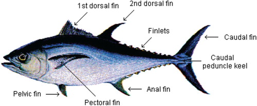
Maximum fork length is about 100 cm and weight about 13.6 kg, common to 60 cm. The all-tackle angling record is a 11.80 kg fish taken in 1980 from Merimbala, New South Wales, with a fork length of 96.5 cm. In Philippine waters, maturity is attained at about 40 cm fork length, while in the Arabian Sea it is reached between 50 and 65 cm in the third year of age.

3. Geographical distribution

Because of different distributions due to their specific thermal tolerances and as they are exploited by different fisheries, a distinction is made between tropical and temperate tunas. Tropical tunas are found in waters with temperatures greater than 18°C (although they can dive in colder waters) whereas temperate tuna are found in waters as cold as 10°C, but can also be found in tropical waters (Brill 1994). Little tuna is found throughout the warm waters of the Arabian Sea, Indo-West Pacific, including oceanic islands and archipelagos. A few stray specimens have been collected in the eastern tropical Pacific.

4. Habitat and biology

Little tuna is an epipelagic, neritic species inhabiting water temperatures from 18 to 29°C. Like other scombrids, E. affinis tend to form multispecies schools by size, i.e. with small Thunnus albacares, Katsuwonus pelamis, Auxis sp., and Megalaspis cordyla (a carangid), comprising from 100 to over 5000 individuals. Although sexually mature fish may be encountered throughout the year, there are seasonal spawning peaks varying according to regions: i.e. May to September in Arabian Sea, March to May in Philippine waters; during the period of the NW monsoon (October–November to April–May) around the Seychelles; from the middle of the NW monsoon period to the beginning of the SE monsoon (January to July) off East Africa; and probably from August to October off Indonesia.

The only available information on fecundity applies to Arabian Sea material: a 1.4 kg female (48 cm fork length) spawns approximately 0.21 million eggs per batch (corresponding to about 0.79 million per season), whereas a female weighing 4.6 kg (65 cm fork length) may spawn some 0.68 million eggs per batch (2.5 million per season). The sex ratio in immature fish is about 1 : 1, while males predominate in the adult stages. E. affinis is a highly opportunistic predator feeding indiscriminately on fish, shrimps and cephalopods. In turn, it is preyed upon by marlins and sharks.

5. Global capture production for Euthynnus affinis

World little tuna fisheries are reviewed in terms of commercially important species, by ocean and by major fishing gear types. Little tuna are very important economically and are a significant source of protein food. The reported world catch (eight countries) for the period between 1975 and 1981 fluctuated between about 44,000 and 65,000 t per year (Figure 2). The 1977 catches were exceptionally high, almost 84,000 t. About 67,500 t were reported for 1981 (FAO 2008). The countries with the largest landings were the Philippines, Malaysia and India.

Figure 2. Global trends in little tuna (Euthynnus affinis) capture production.

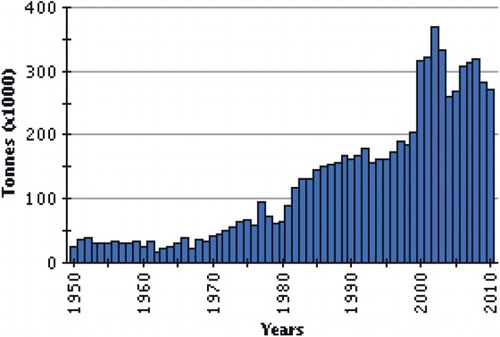
In Pakistan, E. affinis is an important species in local drift net (gillnet) and hook and line fisheries, even though this country has not supplied separate statistics for it during the above period. Typically these are multispecies fisheries also taking E. affinis. Besides gillnetting, trawling is the major fishing technique in use. Occasionally beach seines and longlines are also deployed. Some gear types are rather size-selective, i.e. trawling lines take smaller fish than gillnets. The meat is of good quality when fresh, but it deteriorates very fast if not treated adequately. The total catch reported for this species to FAO for 2009 was 169,607 t. The countries with the largest catches were Malaysia (57,281 t) and Thailand (45,768 t). Their global production has tended to increase continuously from less than 170,000 t in 2009 to above 200,000 t in 2011. They are landed in many locations around the world, traded on a nearly global scale and processed and consumed in many locations worldwide. Generally, tuna catches have had an uncertain pattern – flat, or in some cases decreasing. However, between 1997 and 2009 catches increased by about 19% due to an abundance of skipjack, especially in the Pacific Ocean. Most catches of the principal market tuna species in 2008 were caught from the Pacific (70.2%) followed by Indian Ocean, which contributes much more (20.4%) than the Atlantic (8.0%) and the Mediterranean Sea (1.4%).

6. Study area

Pakistan is largely arid and semi-arid, receiving less than 250 mm annual rainfall, with the driest regions receiving less than 125 mm of rain annually. It has a diverse landscape, with high mountain systems, fragile watershed areas, alluvial plains, coastal mangroves, and dune deserts. Pakistan has a coastline of about 990 km and an exclusive economic zone (EEZ) of about 240,000 km². It roughly divided into two main sections on the basis of its physiographical characteristics, namely the Sind coast and the Baluchistan coast. The Sind coast is roughly 320 km long with continental shelf deep stretches into the ocean, and is located in the south-eastern part of the country between the Indian border along Sir Creek on the east, while the Baluchistan coast is 670 km long with steep and narrow continental shelf at south-western part of the country and borders with Iran near Jiwani in the west (UNEP 1990). The Pakistan coastline is shown in Figure 3.

Figure 3. Map showing the Pakistan coastline.

Source: NIO Technical Report, 1996. National Institute of Oceanography, NODC, Karachi, Pakistan.

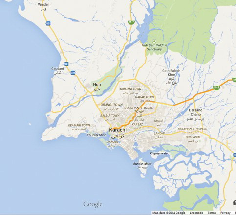
Karachi in Pakistan is located on the northern border of the Arabian Sea and its population is over 18 million. Existing estimates show that mangroves cover approximately 129,000 hectares in the Indus Delta and about 3000 hectares on the Balochistan coast in the Miani Hor, Kalmat Khor, and Gawadar Bay areas. Heavy metals are the major component of the waste effluents discharged from Karachi municipality. The UNEP in its regional seas program in 1989 has included Pakistan in a group of countries which are vulnerable to rising sea levels. Historical air temperature and sea surface temperature (SST) data of Karachi also show increasing patterns; there has been an increase of about 0.67°C in air temperature over the last 35 years. The mean SST in the coastal waters of Karachi has also increased by about 0.3°C in a decade.

The Sindh coastal zone is more vulnerable to sea level rise than the Balochistan coast, as the Balochistan coast shows uplifting by about 1–2 mm year^–1 due to subduction of the Indian Ocean plate. Within the Indus deltaic creek system, the area near Karachi is more vulnerable to coastal erosion and accretion than the other deltaic region, mainly due to human activities together with natural phenomena such as wave action, strong tidal currents and rises in sea level. The increasing pattern in sea level about 1.1 mm year–1 at Karachi Harbor has been taken as a base reference to study the impact of sea level rise along Pakistan coast. A graphical representation of tidal behavior with the trend line is shown in Figure 4. As the rate of increment in sea level at Karachi is within the global range, the rate may be treated as a eustatic sea level rise, i.e. the rise is due to thermal expansion of sea water. However, the higher base provided by SLR for storm surges and tides would be particularly important for the Indus delta, where the beach slope is only about 0.1° (Wells and Coleman 1985). A synoptic view of the Indus delta is shown in Figure 5.

Figure 4. Sea level trends along the Karachi coast, Pakistan.

Figure 5. Map of Karachi coast. Source: © Google Map Data 2014. Downloaded 20 October 2014.

7. Material and methods

7.1. Sampling point and sample collection

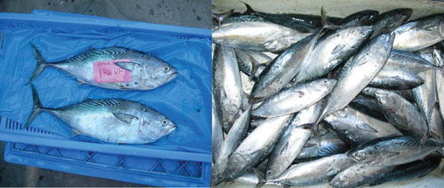
Samples of fishes were collected seasonally (autumn, winter, spring, summer) from Karachi coast, Fish Harbor West Wharf, Karachi (Figure 5). Fishes were collected during seasonal surveys as follows: autumn (September and October), winter (November, December and January), spring (February and March), and summer (April, May, June and July) between August 2006 and December 2011. In 2006–2007, 54 Euthynnus affinis were collected; 61 in 2007–2008; 56 in 2008–2009; 52 in 2009–2010; and 55 in 2010–2011. Data from all major tuna fish landing centers in different sampling stations of the Karachi coast were collected and raised to monthly and annual figures using the Stratified Random Sampling Technique developed at Department of Zoology, University of Karachi, Pakistan. The state figures were then added to get the total landings of the country. Length measurements (fork length) were also taken at the landing stations and were raised to the monthly/annual catches. These formed the basic data for estimating the growth and population structure of E. affinis using length based models. Random samples were collected from the commercial landings and transported to the laboratory for further biological studies.

7.2. Sample preservation

Fish samples were immediately transported to the laboratory, thawed and rinsed in distilled water to remove foreign particles, then length (cm) and weight (g) were determined. Fish were tagged for identification and then stored at 4°C until time for analysis.

7.3. Length (cm) and weight (g) of fishes

The length (L) of the fish was measured from the tip of the anterior part of the mouth to the caudal fin in centimeters (Figure 6). Fish weight was measured after blot drying with a piece of clean towel. From the fresh samples, total length (TL, cm) and body weight (W, g) were measured to the nearest 0.1 cm and 0.01 g, respectively. The fork length (cm) and wet weight (g) were taken and used to calculate the length–weight relationship using the method suggested by Le Cren (1951). The fish was then cut open, and its sex and gonad maturity stage identified. Structure and size of gonads were observed and classified as per the ICES scale adopted by Wood (1930). Size at first maturity was determined as suggested by Lockwood (1988) and King (2013). For the purpose of fecundity studies, fishes in stages IV and V alone were considered. Mature ova were counted and the total fecundity was estimated using the formula:

Stomachs were carefully removed and food contents studied in detail to understand the food and feeding habit of E. affinis. Stomach fullness was visually classified into five categories as full, three-quarters full, half full, one-quarter full and empty based on the distension of the stomach due to the presence or absence of food. The average intensity of feeding was evaluated by point's method (Bapat and Bal 1952; Hynes 1950). The different items constituting one category were sorted and counted. For each item, identifiable organs were used to determine the number of prey present in the stomach. Prey was identified up to genus level and further to species level whenever possible using keys and descriptions found in Fischer and Whitehead (1974) and Smith (2003) and by comparison with material available in our reference collection at the Institute. Growth parameters, i.e. asymptotic length (L∞) and growth co-efficient (K), were estimated using the ELEFAN I module of FiSAT software and the Powell-Wetherall plot (Gayanilo Jr et al. 1996). The length based growth performance index Ø was calculated from L∞ and K. The probability of capture and size at first capture (Lc) were estimated as in Ingles and Pauly (1984) and the age at zero length (t0) from empirical equation. Longevity was estimated from tmax = 3/K + t0.

Natural mortality (M) was calculated by Pauly's empirical formula (Ingles and Pauly 1984) and total mortality (Z) from length converted catch curve. Length structured virtual population analysis (VPA) was used to obtain fishing mortalities per length class. Exploitation rate was estimated from the equation, E = F/Z and exploitation ratio from U = F/Z*(1-e-z); where F is the fishing mortality rate.

Total stock (P) and biomass (B) were estimated from the ratios Y/U and Y/F respectively; where Y is the annual average yield in tonnes. Maximum sustainable yield was calculated as for exploited fish stocks. The relative yield per recruit (Y/R) and biomass per recruit (B/R) at different levels of F were estimated using (Beverton and Holt 1959) model FiSAT software (Gayanilo Jr et al. 1996; Figure 6).

Figure 6. Little tuna (Euthynnus affinis) samples collected from Karachi coast.

7.4. Sample preparation for elemental analysis

Samples were collected for the analysis of heavy metals. Fishes were dissected using steel scissors and scalpels to remove approximately 5 g dorsal muscles, the entire liver, two rakers of gills, entire kidney, and entire gonads. These were washed with deionized water and weighed (Tüzen 2003; Karadede et al. 2004; Papagiannis et al. 2004). Samples were ground and calcinated at 500°C for 3 h until it turned to white or gray ash. The ashes were dissolved with 0.1 M HCl according to the method of Gutierrez et al. (1989). The ashes were dissolved in 10 ml (HCl) in a beaker, after which the dissolved ash residue was filtered with Whatman filter paper. The filtered solution then diluted with 25 ml distilled water for elemental analysis.

7.5. Analysis of sample on atomic absorption spectrophotometer

A 1 ml aliquot of the prepared sample was diluted in 25 ml of distilled water. Three standards, of 2, 4 and 6 ppm, were prepared from 1000 ppm stock solution and used to calibrate the equipment. 1 ml aliquot of the prepared sample was diluted in 25 ml of distilled water. The diluted sample then analysed by atomic absorption spectrophotometer. Three standards, of 2, 4 and 6 ppm, were prepared from 1000 ppm stock solution and used to calibrate the equipment. The samples were aspirated one by one to detect the required metals. Finally, the software was used to prepare the report.

7.6. Risk assessment criteria

Two main criteria were employed when reviewing available data to select the specific data to be used in this study: (1) sampling must have been conducted in the study area; and (2) the species and edible matrix of fish consumed by anglers must have been represented in the analyses. The first criterion is straightforward, whereas the second is based upon the extensive creel angler survey (CAS) conducted in the study area, thus providing very detailed information about fish consumption patterns (Ray et al. 2007). Results of the CAS indicated that there were Euthynnus affinis fish consumed by anglers and that the majority of anglers along the coast consumed fish fillets with skin off. Responses from CAS interviews indicated that data to be utilized in a human health risk assessment associated with consumption of coastal fishing should be based on concentrations measured in fillets without skin from fish species typically consumed by coastal anglers. In fact, the CAS found that more than 95% of the area's angler population intercepted for the study that consumed their catch (less than 9% of all anglers interviewed) ate only fish fillets (skin on or off) (Ray et al. 2007). These results conform to the USEPA recommendation to use composites of fillets in screening studies to provide conservative estimates of typical exposures for the general population (United States Environment Protection Agency (USEPA) (2000).

7.7. Evaluation of publicly available database

Initially, a general review of the types of data contained within the database available at the Department of Marine Fisheries (DMF), West Wharf, Karachi was conducted. The format, usability, and supporting data varied greatly both within and between the databases. Using the assessment criteria described above, a preliminary evaluation found that the DMF database meets the above criteria, and as a result all analyses reported in this study were based on data maintained by USEPA.

The database contained different tables that provided information on many types of media, measurements of hundreds of analytes, and associated metadata (e.g. sample location, date, analytical limits of detection, etc). Generally, each sample set also had a unique analyte list, unique data quality flags and indicators, and unique detection/quantitation limit information. For the purposes of this paper, ‘sample’ refers to a mass of fish tissue that was extracted and analyzed for chemical concentrations. The stepwise process used to reduce the data to a format usable and applicable for risk assessment (Figure 7) is described in this section.

Figure 7. Data reduction process for fish tissue.

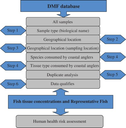
Step 1 – determine sample type

The first step was to determine what types of samples existed in the database. The results from this query indicated that three of the eight listed sample types were biological in nature: ‘bioaccumulation,’ ‘biological tissue chemistry’ and ‘biota toxicity.’

Step 2 – determine geographical location

Latitude and longitude information was extracted for each unique biological sample and each sample location was plotted in ArcGIS version 9.2. Sample IDs associated with biological tissue samples from the study area were then extracted from the geographic information system (GIS). These study area-specific sample IDs were then used to screen the biological samples identified in Step 1 and extract analytical results representative of samples collected from the area.

Step 3 – data quality evaluation

Duplicate samples and samples of unknown quality control (QC) status were then removed from the dataset.

Step 4 – apply area consumption patterns

Data were reduced further to reflect fish consumption patterns of anglers based upon the findings of the CAS conducted in 2000–2001 (Ray et al. 2007). Data were available in the Department of Marine Fisheries (DMF) database for four of the five species identified in the CAS; thus the dataset was reduced again to reflect only species demonstrated to be consumed by anglers in the study area. The remaining samples then were reduced further by sample type so that only ‘fillet’ data remained.

Step 5 – eliminate reanalysis results

For some analyte measurements, there were multiple analyses conducted with different detection limits. Only one of the two analyses was selected using the following decision framework: if both analyses were not detected, the lower detection limit was selected; if both analyses were detected, the results were averaged; if one analysis was detected and one was not detected, the detected analysis was selected. Additionally, some analytes were measured using multiple methods. To ensure that a given analyte was not accounted for more than once, a single metric was selected and remaining duplicative analyses were omitted.

Step 6 – evaluate data qualifiers

Many of the results contained data qualifiers based upon the analysis. Quality assurance (QA) and QC indicator flags for the samples were found to be a product of two processes: QC checks conducted by the laboratory or by an independent data validation contractor. A concentration equal to the sample quantitation limit (SQL) was reported as a proxy value for analyte concentrations characterized as being below the method detection limit (MDL) because MDL values were not included in the database. The SQL of an analyte is typically greater than its MDL, and therefore provides a conservative approach to characterizing analyte concentrations in the absence of measurable data. Remaining data were then extracted by species and matrix for each ingested species in the CAS. Data were sorted by sample ID, and then by analyte.

7.8. Representative fish calculation

The Representative Fish parameter takes into account several variables: (1) the edible matrix (i.e. fillet) of the fish consumed by anglers; (2) the specific species consumed by anglers; (3) the proportional consumption of little tuna; and (4) the concentration of all contaminants in tuna fish. Representative Fish concentrations were calculated using a weighted average approach depicted by Equation (1):

where C is concentration and ‘Mass’ is the weight of the fish sample. The MFD CAS specifies an annual population ingestion rate in grams (g) for little tuna (Ray et al. 2007). Thus, the sum of all reported specific ingestion rates was used in calculating the proportion of each fish for the Representative Fish parameter. The final proportion of the tuna which comprise the Representative Fish was: 97% little tuna (fillet skin off), and 3% little tuna (fillet, skin on). Fillet samples without skin were preferred since the CAS results demonstrated that this was the method of preparation utilized by most of the fish consuming anglers.

7.9. Calculation of summary statistics

Descriptive statistics (mean, standard deviation, range) and three-way analysis of variance (ANOVA) were conducted using Excel spreadsheet. The data transformations allowed for adjusting of all the zero values in the analytical results prior to the ANOVA test. A three-way ANOVA statistical procedure was employed in the assessment of variation in metal concentrations. Three-way ANOVA in which the within-sample variances and between-sample variances were considered was used to test for the significance of differences between organs and between metals. The three-way ANOVA method was also used to consider the first-order interactions between the three factors, namely organs, year and seasons. The Bonferroni test was used for correction to counteract the problem of multiple comparisons.

Summary statistics were calculated on a wet weight basis for all samples in the reduced dataset. These samples were composite samples rather than individual fish samples. However, the number of fish in a composite, the mass contribution of each fish in a given composite, as well as the total mass of each composite was variable. Because of the complexity of developing an analytical solution to this three-variable system, we took the general view that composite samples are ultimately an estimate of the mean concentration.

8. Result and discussion

8.1. Fishery

E. affinis was exploited mainly by crafts using a combination of gillnets (56%) and hooks and lines (23%). Gillnets and hooks and lines operated separately also contributed significantly to the catch. Ring seines, purse seines and trawls landed this species occasionally. The catch by other gears including shore seines and smaller monofilament trammel nets was insignificant (Figure 8).

Figure 8. Contribution (%) of different gears to total E. affinis catch.

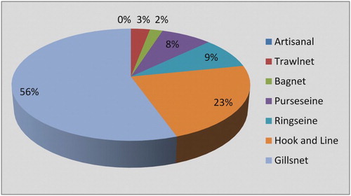
Figure 9. Annual landings of E. affinis during 2006–2013.

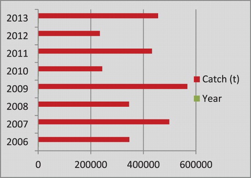
The annual catches of E. affinis during 2006–2013 (Figure 8) ranged between 29,939 t (2007) and 56,322 t (2008), with an average catch of 40,757 t forming 63.6% of the coastal tuna catches and 20.7% of the total tuna catch of the country. Thereafter the catch registered a decline and remained around 10,500 t. The decline was observed in all the gears exploiting E. affinis.

8.2. Seasonal abundance

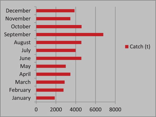
Landing of E. affinis was observed throughout the year with a peak during September–October (Figure 10) when 40.7% of the catch was landed. A second smaller peak was observed during December. The annual average monthly catch of E. affinis was highest in September (7758 t) followed by June (4858 t) and October (42,442 t). September was the most productive month along the Karachi coast.

Figure 10. Seasonal trends in landing of E. affinis.

8.3. Length composition

The reproductive characteristics of a stock along with those of growth and mortality are among the most important factors in determining the regenerative ability of a population (Quinn and Deriso 1999b). The length ranged from a minimum of 14 cm to a maximum of 80 cm. States along the east coast recorded a wide range of length distribution (Figure 11, Table 1). Fishes in the length range of 34–54 cm dominated the catch and contributed 70% of the catch. Major modes were at 50 and 40 cm and the annual mean length of E. affinis landed for all states combined was 45.9 cm.

Figure 11. Length–frequency distribution of E. affinis in the fishery.

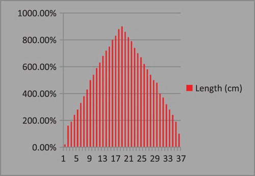
Table shows the length–weight relationship of little tuna caught from the Arabian Sea, including a comparison of the length–weight relationship observed in different studies. The data for length–weight relationship of little tuna with respect to the stock occurring in the Arabian Sea is available (Dissanayake et al. 2008; Morita 1973; Pillai et al. 1993). Newly recruited fish are primarily caught by purse seine fishery on floating objects. Males are predominant in the catches of larger fish, with sizes more than 140 cm (this is also the case in other oceans). The length–weight relationships calculated are: male: W = 0.00001 L 3.25 (r = 0.96); female: W = 0.00001 L 3.01 (r = 0.98); pooled: W = 0.00001 L 3.09 (r = 0.96). The length–weight relationship of little tuna from the Indian Ocean was studied by Hsu (1999) and was determined using data from gillnet catches. Altogether 2499 specimens were measured, with a range of FL 46.2–112 cm and a length–weight relationship W = 0.056907 FL2.7514. The length classes of 102.5–117.5 cm were observed to peak from January to April and those of 92.5–97.5 cm to peak from October to December (Dissanayake et al. 2008).

The von Bertalanffy growth curve is FL = 168.99 (1-e-0.000879(t + 123.38)), where FL is in centimeters and t is in days (Table 2). The results obtained with spines and otoliths are comparable until three years old, but spines are not suitable for larger fish (Stequert and Conand 2003; Farley et al. 2006), so information on the age and growth of bigeye tuna in the eastern and western Australian fishing zone is based on otoliths. The fishery, population characteristics and stock estimates of frigate tuna from Indian waters were studied during 2006–2010 by Ghosh (2012). Length at first maturity was estimated as 29.7 cm and fecundity was observed as 807.98 kg/body weight. The von Bertalanffy growth equation derived was Lt = 57.95 [1-e-1.2(t + 0.0075)]. The growth parameters, L∞ and K, were estimated at 57.95 cm and 1.2 year^–1. Growth performance index was 3.605, t 0−0.0075 and the length at first capture was 32.83 cm. The natural mortality, fishing mortality and total mortality were 1.65, 3.24 and 4.89 year^–1 respectively and with an exploitation ratio of 0.66. Emax was estimated as 0.778, which is higher than the present exploitation, indicating scope for further exploitation. Pillai et al. (2002a) studied population characteristics and stock status of little tuna in Arabian waters. The growth parameters, L∞ and K, were estimated at 37.00 cm and 0.638 year^–1. The natural morality rate M was estimated 1.024 year^–1, total mortality Z (2.739 year^–1), fishing mortality F (1.7147 year^–1), and exploitation rate U (0.74) from the Arabian Sea. Estimates of exploitation rate of bullet tuna indicate that they are exploited below the optimum level (IOTC 2011). Above findings suggests that there is considerable scope for improving their production.

Table 1  Length and weight and seasonal distribution of Euthynnus affinis samples (X, SD = deviation, N = number of samples).

Table 2  Bonferroni test fish Euthynnus affinis collected from Karachi coast.

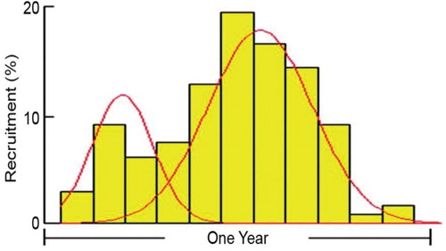
8.4. Maturity, fecundity, spawning and recruitment

Minimum size at maturity was fixed at the length when 50% of the fishes were found to be mature. The size at first maturity for E. affinis was estimated at 37.7 cm (Figure 12). Spawning was observed round the year with peaks during June and October. Two peaks in recruitment were also observed. The major recruitment period was during October–December and the second minor peak was observed during February–April (Figure 13). The first pulse contributed 59.25% and the second 22.85% of recruits. The fecundity was estimated at 308,150 eggs per kg body weight.

Figure 12. Observed and estimated size at first maturity for E. affinis.

Figure 13. Recruitment pattern in E. affinis.

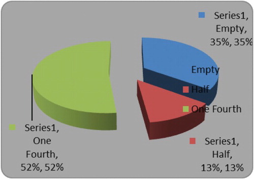
8.5. Food and feeding

Feeding intensity was generally low for the species with none of the sampled fish having a gorged or full stomach condition. Stomach with one-quarter fullness formed the dominant group and contributed 52%. Fishes with empty stomachs formed the next dominant group, followed by fishes with half-full stomachs (13%) (Figure 14).

Figure 14. Feeding intensity (stomach condition) of E. affinis.

Feeding habit indicated E. affinis to be a non-selective generalist feeder, foraging mainly on fin fishes, crustaceans and mollusks (Figure 15). Fishes formed the dominant prey item and contributed 75% of the diet consumed.

Figure 15. Major food groups constituting the diet of E. affinis.

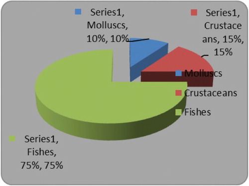
Sardinella longiceps (27.4%), Encrasicholina devisi (24.7%), Decapterus spp. (13.7%) and Nemipterus spp. (3.22%) were the major food items constituting the fish diet. Partially digested fish parts formed 4.99% of the diet. The crustacean component mainly comprised partially digested limbs which formed 13.7% of the total diet. Mollusks were represented entirely by squids (Loligo spp.) and formed 9.6% of the diet.

8.6. Growth

The reproductive characteristics of a stock along with those of growth and mortality are among the most important factors in determining the regenerative ability of a population (Quinn and Deriso 1999a).The length–weight relationship for E. affinis estimated using the method suggested by (Le Cren 1951) was W = 0.0254 L 2.889, where W is the weight of fish in grams and L is fork length in centimeters. The different growth parameters in the von Bertalanffy growth equation Lt = L∞ [1−e k (t−t0)] was Lt = 81.92 [1−e−0.56(t−0.0317)]. The asymptotic weight was 8563 g and size at first capture (Lc) was 41.43 cm at an age (tc) of 2.1 years. The growth performance index was 3.34. The longevity of E. affinis was 9.03 years and the length attained by the fish at the end of the first and second years was 42.7 and 59.5 cm respectively. Fishery was sustained mainly by the 1 to 2 + yr old fishes(34–50 cm).

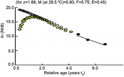
8.7. Mortality, exploitation and virtual population analysis (VPA)

The natural mortality rate (M), fishing mortality rate (F) and total mortality rate (Z) computed were 0.93, 0.75 and 1.68, respectively (Figure 16). The exploitation ratio was 0.45 and exploitation rate was 0.36. Emax was estimated as 0.811 which is much higher than the present exploitation, indicating further scope for exploitation of this species.

Figure 16. Mortalities and exploitation rate of E. affinis estimated using length converted catch curve.

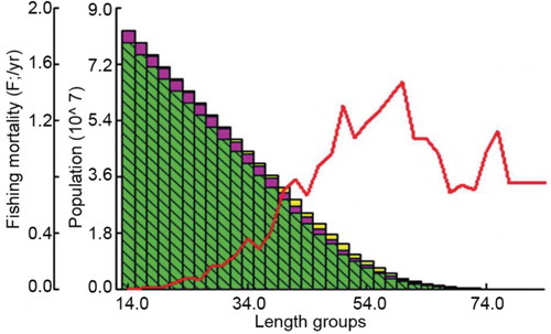
Virtual population analysis (VPA) indicated that main loss in the stock up to 32 cm size was due to natural causes (Figure 17). Fishes became more vulnerable to the gear after this size and mortality due to fishing increased. However, loss due to fishing remained very low (Figure 17).

Figure 17. Virtual population analysis of E. affinis.

8.8. Stock and maximum sustainable yield (MSY)

The annual total standing stock, biomass and MSY of E. affinis were estimated at 112,208, 54,342 and 45,647 t, respectively. The average annual yield was 40,757 t.

8.9. Yield/recruit

The yield and biomass/recruit and yield and biomass curves showed that the maximum yield and yield/recruit could be obtained by increasing the present level of fishing from 1 to 2.2 (Figure 18). The maximum yield and yield per recruit obtained by increasing the present fishing effort by 2.2 times is 47,966 t and 509.31 g, whereas at the present level of fishing, it is 40,757 t and 432.76 g (Figure 14 and 15). The increase in relative yield at the increased effort would be 117.7%.

Figure 18. Yield per recruit and biomass per recruit curves for E. affinis.

8.10. Seasonal elemental variations

8.10.1. Cadmium

The maximum mean concentration of Cd (2.21 ± 0.80 µg g^–1 dry weight [dw]) was recorded in liver during spring season (2010–2011) and the second highest mean (1.81 + 0.66 µg g^–1 dw) was recorded in liver during autumn season (2009–2010). The lowest mean concentration in liver (0.56 + 0.51 µg g^–1 dw) was recorded in winter 2010–2011, and the second lowest mean (0.60 + 0.59 µg g^–1 dw) was recorded in spring 2008–2009. The highest mean concentration in muscle (0.50 + 0.17 µg g^–1 dw) was recorded in summer 2010–2011 and the second highest (0.48 + 0.28 µg g^–1 dw) was recorded in summer 2009–2010. The lowest mean concentration in muscle (0.14 + 0.12 µg g^–1 dw) was recorded in winter 2006–2007 and the second lowest (0.19 + 0.14 µg g^–1 dw) was recorded in autumn 2007–2008. The highest mean concentration in kidney (0.41 + 0.18 µg g^–1 dw) was recorded in autumn 2010–2011 and the second highest mean concentration (0.36 + 0.20 µg g^–1 dw) was recorded in winter 2010–2011. The lowest mean concentration in kidney (0.06 + 0.05 µg g^–1 dw) was recorded in autumn 2006–2007 and the second lowest mean concentration (0.06 + 0.05 µg g^–1 dw) was recorded in winter 2006–2007. The highest mean concentration in gills (0.64 + 0.25 µg g^–1 dw) was recorded in spring 2009–2010 and the second highest (0.59 + 0.15 µg g^–1 dw) was recorded in autumn 2009–2010. The lowest mean concentration in gills (0.23 + 0.22 µg g^–1 dw) was recorded in spring 2006–2007 and second lowest (0.25 + 0.14 µg g^–1 dw) was recorded in winter 2006–2007. The highest mean concentration in gonads (0.63 ± 0.12 µg g^–1 dw) was recorded in spring 2009–2010 and second highest (0.53 ± 0.23 µg g^–1 dw) was recorded in winter 2009–2010. The lowest mean concentration in gonads (0.11 ± 0.07 µg g^–1 dw) was recorded in winter 2006–2007 and second lowest mean concentration (0.15 ± 0.14 µg g^–1 dw) was recorded in autumn 2007–2008 (Tables and ).

8.10.2. Lead

The highest mean concentration of Pb (1.58 ± 0.32 µg g^–1 dw) was recorded in liver during summer season (2010–2011) and the second highest mean (1.49 ± 0.17 µg g^–1 dw) was also recorded in liver during summer season (2008–2009). The lowest mean concentration in liver (1.21 ± 0.32 µg g^–1 dw) was recorded in autumn 2007–2008 and the second lowest mean (1.21 ± 0.36 µg g^–1 dw) was recorded in spring 2006–2007. The highest mean concentration in muscle (0.54 ± 0.15 µg g^–1 dw) was recorded in summer 2009–2010 and the second highest (0.50 ± 0.12 µg g^–1 dw) was recorded in autumn 2008–2009. The lowest mean concentration in muscles (0.06 ± 0.05 µg g^–1 dw) was recorded in winter 2006–2007 and the second lowest (0.10 ± 0.02 µg g^–1 dw) was recorded in autumn 2006–2007.

The maximum mean concentration in kidney (0.63 ±0.12 µg g^–1 dw) was recorded in summer 2010–2011 and the second highest mean concentrations (0.58 ± 0.12 µg g^–1 dw) was recorded in autumn 2010–2011. The lowest mean concentration in kidney (0.11 ± 0.06 µg g^–1 dw) was recorded in winter 2006–2007 and the second lowest mean concentration (0.13 ± 0.05 µg g^–1 dw) was recorded in autumn 2006–2007. The highest mean concentration in gills (0.66 ± 0.32 µg g^–1 dw) was recorded in summer 2010–2011 and the second highest (0.54 ± 0.13 µg g^–1 dw) was recorded in winter 2010–2011. The lowest mean concentration in gills (0.21 ± 0.11 µg g^–1 dw) was recorded in winter 2006–2007 and the second lowest (0.21 ± 0.15 µg g^–1 dw) was recorded in autumn 2006–2007. The highest mean concentration in gonads (0.52 ± 0.10 µg g^–1 dw) was recorded in spring 2009–2010 and the second highest (0.51 ± 0.15 µg g^–1 dw) was recorded in autumn 2009–2010. The lowest mean concentration in gonads (0.11 ± 0.07 µg g^–1 dw) was recorded in autumn 2006–2007 and the second lowest mean concentration (0.12 ± 0.10 µg g^–1 dw) was recorded in winter 2006–2007 (Tables and ).

Table 3  Metal concentrations in selected organs of the examined Euthynnus affinis fish from the Karachi coast (2006—2011).

Table 4  Analysis of variance (ANOVA) in Euthynnus affinis fish from the coast of Karachi.

8.10.3. Zinc

The highest mean concentration of Zn (56.33 ± 9.68 µg g^–1 dw) was recorded in liver during spring season (2010–2011) and the second highest mean (54.65 ± 13.83 µg g^–1 dw) was recorded in liver during summer season (2010–2011). The lowest mean concentration in liver (28.13 ± 7.52 µg g^–1 dw) was recorded in autumn 2006–2007 and the second lowest mean (29.81 ± 7.22 µg g^–1 dw) was recorded in spring 2006–2007. The highest mean concentration in muscle (16.33 ± 2.26 µg g^–1 dw) was recorded in summer 2008–2009 and the second highest (15.32 ± 2.94 µg g^–1 dw) was recorded in summer 2007–2008. The lowest mean concentration in muscle (6.56 ± 1.06 µg g^–1 dw) was recorded in autumn 2006–2007 and the second lowest (6.98 ± 1.63 µg g^–1 dw) was recorded in winter 2006–2007.

The highest mean concentration in kidney (16.45 ±6.85 µg g^–1 dw) was recorded in summer 2010–2011 and the second highest mean concentration (16.28 ± 2.70 µg g^–1 dw) was recorded in summer 2008–2009. The lowest mean concentration in kidney (6.49 ± 1.72 µg g^–1 dw) was recorded in autumn 2006–2007 and the second lowest mean concentration (8.24 ± 0.85 µg g^–1 dw) was recorded in summer 2006–2007. The maximum mean concentration in gills (16.34 ± 5.13 µg g^–1 dw) was recorded in autumn 2010–2011 and the second highest (16.34 ± 2.40 µg g^–1 dw) was recorded in winter 2010–2011. The lowest mean concentration in gills (5.62 ± 0.83 µg g^–1 dw) was recorded in winter 2006–2007 and the second lowest (6.23 ± 1.10 µg g^–1 dw) was recorded in winter 2008–2009. The highest mean concentration in gonads (7.47 ± 1.33 µg g^–1 dw) was recorded in summer 2010–2011 and the second highest (7.03 ± 1.47 µg g^–1 dw) was recorded in summer 2008–2009. The lowest mean concentration in gonads (4.13 ± 0.72 µg g^–1 dw) was recorded in winter 2006–2007 and the second lowest mean concentration (4.24 ± 0.97 µg g^–1 dw) was recorded in autumn 2006–2007 (Tables and ).

8.10.4. Copper

The maximum mean concentration of Cu (59.07 ± 24.59 µg g^–1 dw) in liver was recorded in autumn 2010–2011 and the second highest mean (51.61 ± 21.65 µg g^–1 dw) was recorded in summer 2010–2011. The lowest mean concentration in liver (27.12 ± 21.23 µg g^–1 dw) was recorded in autumn 2007–2008 and the second lowest mean (31.21 ± 10.34 µg g^–1 dw) was recorded in spring 2006–2007. The highest mean concentration in muscle (6.63 ± 1.65 µg g^–1 dw) was recorded in summer 2010–2011 and the second highest (5.44 ± 2.41 µg g^–1 dw) was recorded in summer 2009–2010. The lowest mean concentration in muscles (2.36 ± 1.78 µg g^–1 dw) was recorded in summer 2007–2008 and the second lowest (2.38 ± 1.86 µg g^–1 dw) was estimated in autumn 2006–2007.

The highest mean concentration in kidney (19.46 ±4.29 µg g^–1 dw) were recorded in summer 2007–2008 and the second highest mean concentration (19.39 ± 5.26 µg g^–1 dw) was recorded in spring 2007–2008 (Table 3). The lowest mean concentration in kidney (7.67 ± 3.94 µg g^–1 dw) was recorded in winter 2006–2007 and the second lowest mean concentration (9.11 ± 3.51 µg g^–1 dw) was recorded in spring 2006–2007. The highest mean concentration in gills (16.57 ± 3.40 µg g^–1 dw) was recorded in spring 2010–2011 and the second highest (16.56 ± 3.54 µg g^–1 dw) was recorded in autumn 2008–2009. The lowest mean concentration in gills (8.30 ± 3.56 µg g^–1 dw) was recorded in winter 2006–2007 and the second lowest (11.71 ± 4.05 µg g^–1 dw) was recorded in autumn 2006–2007. The maximum mean concentration in gonads (9.68 ± 2.86 µg g^–1 dw) was recorded in summer 2010–2010 and the second highest (6.37 ± 1.88 µg g^–1 dw) was recorded in winter 2009–2010. The lowest mean concentrations in gonads (2.40 ± 1.20 µg g^–1 dw) was recorded in summer 2007–2008 and the second lowest mean concentration (2.55 ± 1.03 µg g^–1 dw) was recorded in winter 2007–2008 (Table 3 and Table 4).

Zn has a multitude of biological functions in the human body. It is an important constituent of over 100 enzymes involved in a variety of fundamental metabolic processes. It is involved in the production and function of several hormones. Excessive intake of Zn causes abdominal pain, violent vomiting, collapse, and degenerative changes in the liver. Cu is probably a functional constituent of all cells. Toxicity can result from excessive intake, leading to gastrointestinal disturbance, headache, cirrhosis, necrosis, and liver failure. Cd is considered the most toxic element to human life. It causes itai-itai, a bone disease similar to rickets, and cardiac enlargement, anemia, gonadal atrophy, kidney failure, and pulmonary emphysema. Pb is toxic and a major hazard to man and animals. Poisoning by lead causes anemia, encephalopathy, weight and coordination loss, abdominal pain, vomiting, constipation, and insomnia (Khallaf et al. 2003). Being nonbiodegradable, unlike many organic pollutants, metals can be concentrated along the food chain, producing their toxic effects at points often far away from the source of the pollution (Fernández et al. 2000). Accumulation of heavy metals in the food web can occur either by accumulation from the surrounding medium, such as water or sediment, or by bioaccumulation from the food source (Tulonen et al. 2006). Aquatic organisms have been widely used in biological monitoring and assessment of safe environmental levels of heavy metals. Voegborlo et al. (1999) reported a maximum Cd concentration 0.32 µg g^–1 in canned tuna fish from Libya as against 0.66 µg g^–1 found in Saudian tuna. Tariq et al. (1993) reported 0.35 µg g^–1 Cd in fish of comparable size from the Arabian Sea.

Due to known toxicity of metallic elements in various types of foods that occurs from time to time during commercial handling and processing, most countries monitor the levels of toxic elements in foods. The joint Food and Agricultural Organization/World Health Organization (FAO/WHO) Expert Committee on Food Additives has suggested a provisional tolerable intake of 400–500 µg Cd per week for adult men; the quantity of Hg to be tolerated in human food is 0.3 mg per week and for Pb a weekly intake of 3 mg is allowed. The maximum concentration of lead which is permitted by FAO/WHO in prepared foods specifically intended for babies or young children is 200 µg kg^–1 (CIFA 1992). The US Office of Community and Public Health (OCPH) recommends that people eat a balanced diet, avoiding excessive amounts of tuna. Eating one can per week should not be a problem for pregnant/nursing woman and children under 6 (Zhou et al. 1998).

8.11. Health risk assessment

Step 1 in the risk assessment process (Figure 7) was to extract samples of biological origin from thousands of sample analytes. Evaluation of the geographic location of sampling (Step 2) demonstrated that many of the biological samples in the database were not from the Karachi coastal area but from nearby waterbodies. The GIS results are illustrated in Figure 7. Step 4 represented the most significant elimination of records, reducing the dataset, representing composite samples based upon species-specific consumption patterns of coastal anglers. Of these records, only 587 reflected fillet samples for these species (representing 20 composite samples). The remaining composite samples and records reflect four different sampling events spanning 1995–2001. Different metallic elements were examined in each of the 20 composite samples, including Cd, Pb, Zn and Cu. Further reduction was required on a sample-specific basis to ensure that each analyte was accounted for only once. Step 5 involved eliminating duplicative analyses, reducing the number total number of analytes from 170 to 80 and records from 3000 to 1000, to ensure that all the data were usable based upon laboratory qualifiers. In Step 6 the data qualifiers were evaluated, reducing the total number of records from 1000 to 987. The resulting 987 records and 20 composite samples represented the final dataset, which was used to generate summary statistics and develop the Representative Fish parameter. Generally, samples had very similar analyte lists, sharing most of the common analytes across all the samples. However, the number of samples (n) that were used in the derivation of Representative Fish tissue concentrations varied by analyte because not all samples reported acceptable (i.e. not rejected) concentrations for each of the 156 analytes.

8.12. Fish tissue concentrations and representative fish

Species-specific concentrations for selected analytes are provided in Tables and . Concentrations of the metals generally were measured at levels above the detection limit in a high percentage of samples. Cu was the only nonessential metal detected in 100% of samples analyzed. Pb and cadmium were the only metals with relatively high toxicity factors that had concentrations less than 100 ppb in the Representative Fish. (The approach used herein to identify and select chemical-specific toxicity values, to determine the degree of toxicity, was described previously by Urban et al. 2009.) The 50th and 95th percentile Representative Fish concentrations were calculated for all analytes based upon the species-specific concentrations of each analyte and the proportion of each species consumed by LPR anglers. Representative Fish concentrations are reported for all analytes with usable data, although some values are based upon sample detection limits in cases where analytes were not detected in any sample. Thus, this uncertainty must be considered when these Representative Fish values are applied in fish ingestion human health risk assessments (Urban et al. 2009).

9. Discussion

Tuna fishery in the Arabian Sea is fully developed, with several coastal countries as well as distant water fishing nations participating in the fishery industry. In the Indian Ocean, tuna catches increased rapidly from about 237,986 tonnes in 1980 to 654754 t in 1995. They continued to increase up to 2005; the tuna catch in that year was 1,318,648 t, forming about 26% of the world catch. However, since 2006 onwards there has been a decline in the tuna catch and in 2010 the catch was only 1,257,908 t (Figure 9). Although the catch of little tuna increased gradually in the past five decades, its relative importance decreased rapidly. Gillnets accounted for about 56% of the total tuna catch, followed by hook and line (23%), ring seines (9%), purse seines (8%) and a variety of other gears (5%), as shown in Figure 8.

As many as seven countries have been involved in tuna fishing in the Arabian Sea; the main tuna catching nations are concentrated in Asia, with Taiwan and Japan the main producers. Other important tuna catching nations are the Philippines, Indonesia, South Korea, Spain and France. The present decline in production of the Indian Ocean tuna fisheries may have serious ecological and socioeconomic consequences. Analysis of landing data clearly indicated that over-exploitation of targeted species threatens the sustainability of tuna populations. Though there has been a substantial increase in the production of tunas in the Indian Ocean, the fast pace of development has ignored several patterns which are vital to sustain the tuna production in captured fisheries.

Tuna exploitation in Pakistan has mainly been supported by the smaller coastal species. Of these, E. affinis has been the dominant species distributed along both the coasts of Pakistan as reported earlier (Silas and Pillai 1982; Muthiah 1985; Ganga et al. 2008; Khan 2011). The mode of exploitation of these smaller tunas has remained almost the same over the years, with gillnets and hooks and lines being the main gears used. Availability of E. affinis throughout the year along the east and west coasts has been reported by Kasim and Mohan (2009) and Pillai (2009). Rohit et al. (2012) observed different age classes in the catch, irrespective of season in the Gulf of Aqaba, Red Sea. Balasubramanian and Abdussamad (2007) reported on the availability throughout the year and occurrence of juveniles along Tuticorin coast during June to August which incidentally is the peak fishing season for the species.

Silas et al. (1985) reported that E. affinis fishery along the Indian coast is supported by fishes with a length range of 12–76 cm; later, Mohan Joseph and Jayaprakash (2003) stated that the fishery is supported by fishes with a length range of 10–78 cm. Kasim and Abdussamad (2003) observed that the fishery of E. affinis along the east coast is supported by 18–83 cm length class fishes with 54–56 cm as modal class. The fishery along Maharashtra coast was supported by fishes with a length range of 26–73 cm (Khan 2011). The size range reported earlier is smaller than that observed in the present study, where the fishery was supported by fishes of the size range 14–80 cm. However, the modal length supporting the fishery across the Arabian Sea (34–54 cm) during the study period was much smaller than the modal lengths (50–60 cm) reported by Pillai et al. (2002b) and Kasim and Abdussamad (2003). The modal length was between 34–58 cm and 40–60 cm. Pillai et al. (2003) estimated the size at first maturity (pooled for males and females) as 43–44 cm. Earlier Rao (1964) recorded females of 48 cm with ripe ova near Vizhinjam. Williamson (1970) reported the minimum size at first maturity as 50 cm for E. affinis in Chinese waters. In the Arabian Sea the fish also attained maturity at a total length of 50–65 cm (Williams 1956, 1963a).

In the present study, the size at first maturity estimated for males and females combined was 37.7 cm. The estimated value in the present study is much smaller than the earlier studies but is comparable to that (38.5 cm) reported from Philippine waters (Wade 1950; Ronquillo 1963). Spawning in E. affinis was prolonged with peaks during June and October. James et al. (1993) and Pillai et al. (2003) have made similar observations and noted that the peak spawning for the species may be during October–November and March–June. Muthiah (1985) observed a similar trend for E. affinis from Mangalore coast. Recruitment is a continuous process with two peaks. A bimodal recruitment pattern as observed in the present study has also been reported by Kasim and Abdussamad (2003) along the Arabian Sea. Pillai et al. (2003) reported March and June as the major recruitment period for E. affinis in the Indian seas.

Siraimeetan (1985) studied in detail the food contents of E. affinis from Tuticorin coast and reported that adults fed mainly on fishes while juveniles fed on both fishes and crustaceans (mainly larval stages). Pillai et al. (2003) reported that tunas in general are carnivores and the major food items include crustaceans, cephalopods and fishes. The present study has also found fish to be the major diet of E. affinis, with crustaceans and mollusks forming a less dominant part of the diet. Similar observations of the diet preferences of E. affinis from the Gulf of Aqaba, Red Sea and Eastern Australian waters have been reported (Griffiths et al. 2009). Engraulids were the preferred diet in the present study as well as in the earlier reports. Griffiths et al. (2009) reported that the diet of E. affinis primarily consisted of pelagic clupeids and demersal fish and the smaller fishes fed mainly on small pelagic crustaceans and teleosts.

The length–weight relationship of E. affinis caught from different regions along the Arabian coast has been estimated by several earlier workers and the values obtained (Tables~ and~) are comparable. The fish exhibited isometric growth with the value close to 3. Earlier studies of the growth of E. affinis from different regions have indicated that growth, as in most tuna species, is fast, with the fish having longevity of 2–8 years. Growth parameters in the von Bertalanffy equation as estimated by earlier studies and the present study are given in Table . E. affinis is a fast-growing fish attaining a maximum length of around 80 cm. The L∞ estimated by earlier workers is comparable to the estimate obtained in the present study. The values ranged from 81 to 89 cm. The ‘k’ value however, showed a wide range (Table 2) between 0.35 and 0.9, indicating variations in the length attained in different years. All studies however indicate E. affinis to be fast-growing species, attaining a length of 31–44 cm in the first year. In the present study, E. affinis with a size range of 15–20 cm was observed in the fishery from June to December. These recruits are from the first spawning peak during June–October which lasts for about 2–3 months. A total length of around 40–45 cm at the end of one year is quite expected. Growth parameters obtained in the present study indicated a similar trend in growth with longevity of 5.4 years. The mortality and exploitation rates of E. affinis from different regions are presented in Figure 16. Pillai et al. (2003) stated that the fishery of E. affinis is confined to inshore areas and is exploited to the maximum, which could be why the catches have stabilized. However, values calculated for the Arabian Sea in the present study showed that the present exploitation rate is well within limits of a healthy stock condition. A similar observation was made by James et al. (1993). The exploitation rate is low and preset yield is less than the estimated MSY. Further, the yield per recruit analysis indicated substantial increase in yield with increase in effort (Figure 17). Therefore an increase in effort may be considered to increase the present yield of E. affinis at least to the limit of estimated MSY. However in a multi-fishery scenario, the increase in effort as a management strategy for increasing production of E. affinis needs to be considered cautiously.

The wealth of publicly available monitoring data from sites such as the Karachi coast is a tremendous resource. However, these data can represent many types of media that have been collected, processed, and analyzed by various entities over the past decade, and provide measurements of a wide variety of analytes. Thus, the usability of such data for specific evaluations (i.e. human health risk assessment) first requires rigorous data reduction. The data reduction and resulting findings presented in this study demonstrate the importance of thoroughly reviewing the underlying data in these publicly available datasets as well as applying a consistent and transparent approach to determine analyte concentrations representative of the particular study area of interest.

The resulting analyte records from the data reduction process were used to derive a Representative Fish parameter that can then be applied to risk assessments (Urban et al. 2009). Given the proportional approach to the Representative Fish calculation, the levels of each analyte in the Representative Fish were significantly influenced by concentrations in little tuna. In generating Representative Fish tissue concentrations, the objective was to provide both an estimate of the Clinical Test (CT) and an upper-bound estimate that could ultimately be used in quantitative evaluations of exposure. The basis for determining these concentrations was provided by USEPA (2000), which indicates that the concentration used in exposure equations is the average concentration at the exposure point over the exposure duration. Accordingly, it was important to develop a consistent approach for evaluation of all analytes, species, and matrices for all exposure estimates. For estimates of CT, the median value over all samples was a reasonable selection for two reasons: first, over half of the tissue estimates for a particular analyte, species and matrix combination were proxy values associated with an analytical result of no detection. Therefore, in most cases, estimating a mean was problematic – even with methods that could accommodate non-detected proxy values such as the Kaplan–Meier method in PeocUCL 5.0 US. Second, the median is a good metric for CT for both skewed and symmetric distributions, whereas the mean tends to overestimate or underestimate CT for skewed datasets. In many cases, the skewness associated with an analyte and species for which there are few or no detected concentrations could not be evaluated. In these cases, it was impossible to estimate whether CT would be overestimated using a mean.

Similarly, a consistent approach was sought for estimating an upper-end exposure concentration for the fish species. It was assumed that each composite sample was derived from the distribution of means (i.e. each composite result represented a data point used to generate a distribution of mean concentrations) and the 95th percentile was selected from the distribution of means. In theory, this is similar to conducting a one-tailed 95% upper confidence limit (95% UCL) on the mean; however, estimation of the 95% UCL usually requires knowledge about the variance of the population or the sampling distribution of means. For most of the analytes, there was not a good estimate of this variance because of low sample numbers. Furthermore, the selection of an algorithm to estimate the 95th percentile was also an important consideration. In a situation where there are few data, the decision to interpolate between data points and the methodology by which interpolation is performed can dramatically affect the value that is estimated. Rather than interpolating between data points to estimate a percentile, the empirical cumulative distribution function method was used, in which percentiles are not interpolated between data points, but the next highest data point is selected. The ramification of this decision is that the 95th percentile is represented by the maximum value for the species and matrix sample concentrations available. Although this introduces uncertainty in the resulting estimates of concentration, it is generally conservative in nature and is a transparent and consistent method for developing upper-end estimates of tissue concentrations.

Additional sources of uncertainty in the application of these data in risk assessment involve not only the temporal relation between sampling efforts and evaluation of exposure and risk, but also incomplete evaluations of contaminants. Regarding the issue of temporal relation, fish tissue samples used in the calculation of Representative Fish were collected between 1995 and 2001 and thus are 9–15 years old and may not represent current conditions. As for the issue of incomplete evaluations, the available monitoring data provided in the MFD database are very robust relative to other similar contamination sites, and cover an extensive spectrum of contaminants. However, for the purposes of fish ingestion specific to the lower six miles of the LPR, application of the framework described herein dramatically reduced the number of samples relevant to a human health risk assessment.

A systematic approach to reducing and evaluating the data (based upon site-specific consumption patterns) is necessary prior to conducting risk-based evaluations for the specific area of interest. The data reduction, processing, and analyses that are described in this paper provide a site-specific dataset for use in assessment of human health risk associated with fish consumption, and highlight the importance of thoroughly reviewing the underlying data as well as applying a consistent and transparent approach to determine analyte concentrations representative of the particular study area of interest. Though evaluating the human health risk associated with these analytes was beyond the scope of this study, Urban et al. (2009) have demonstrated, in assessing human health risk associated with consumption of fish, the utility of the data presented in this study. More importantly, however, the step-wise data reduction, processing and analysis approach presented in this study is not limited to the MFD database and this site. Indeed, this approach is a model that should be considered at similar abandoned sites, especially sites where several different parties have supplied large databases of analytical data.

10. Conservation and management

Tunas are like any other renewable living resource; the rate at which they are harvested affects their abundance and their ability to sustain various levels of exploitation. As fishing pressure for tuna increases on a global scale, management and conservation measures are essential if the populations of tunas are to remain at desired levels of abundance. However, the management of tunas is complicated by their migratory nature, and calls for special cooperation among nations, since no one nation can manage tuna effectively. This is reflected in Article 64 of the United Nations Convention on the Law of the Sea, which calls on states to cooperate directly or through appropriate international organizations to ensure the conservation of highly migratory species. The socio-economic importance of tunas coupled with the global spread of industrialized fishing has led to the reduction of global stocks to dangerously low levels (Safina 1998). Recent analyses suggest that large, predatory fishes have declined more than 90% globally in the past 50 years (Myers and Worm 2003), raising concerns regarding the future of many species. This is particularly troubling, as any ecosystem-wide effect is bound to be widespread and likely irreversible due to the global nature of the decline (Myers and Worm 2003).

Maritime countries engaged in fishing tuna and tuna-like species cooperate regarding conservation and fisheries management within several international frameworks (Marashi 1996). Currently there are five regional fisheries management organizations (RFMOs) dedicated to the conservation and management of tunas: the Inter-American Tropical Tuna Commission (IATTC), the Western and Central Pacific Fisheries Commission (WCPFC), the International Commission for the Conservation of Atlantic Tunas (ICCAT), the Indian Ocean Tuna Commission (IOTC), and the Commission for the Conservation of Southern Bluefin Tuna (CCSBT)), whose common objective is to maintain the populations at or above levels of abundance that can support the maximum sustainable yield (MSY). However, as demand for tuna continues to rise, and with it the levels of exploitation, these organizations find it ever more difficult to reach agreement on the implementation of effective management measures. Cooperation must also extend beyond the scale of single oceans. Industrial tuna fleets are highly mobile and in the principle market tunas are intensively traded on a global scale. In addition many tuna research, conservation and management problems are similar in all oceans. Therefore, there is a need for exchange of information and collaboration on a global scale regarding fisheries for tunas and other species with wide global distribution.

11. Major issues in tuna fishery in the Arabian Sea

Tuna fishery in the Arabian Sea is important but not well managed. The evolution of tuna longline fisheries in all oceans has changed fishing strategies, as different species have been targeted. These tactics increase the use of longliners, simultaneously making the stock seem bigger but damaging the breeding capacity of the fish (Botsford et al. 1997). The present study represents an attempt to report the main fishery interaction issues in the Arabian Sea, on the basis of the present knowledge of the fisheries for tuna and tuna-like species. Severe overfishing leads to ecological extinction of species, because overfished populations no longer interact significantly with other species in the community (Jackson et al. 2001). Periodic reassessment of the tuna potential is required, with adequate inputs from exploratory surveys as well as commercial landings; this may prevent any unsustainable trends in the development of the tuna fishing industry in the Indian Ocean.

As many fisheries in the region continue to be open access, i.e. no effective controls are in place to limit the growth of fishing capacity and fishing efforts or to limit catches through a quota regime, the high resource rent potential manifests itself initially in high returns to the owners of fishing vessels. This high profitability attracts new entrants into the fisheries as well inciting current operators to invest in technological improvements of fishing craft and gear, causing the fishing power to increase. The capacity and effort of expanding investments commonly continue to take place until the time when the fishery becomes unprofitable and crew incomes have dropped to a low level.

The economic incentive of the fishery resources in these deeper waters, combined with insufficient monitoring, control and surveillance of fishing activities, has led to a proliferation of illegal, unregulated and unreported (IUU) fishing. IUU fishing activities are now one of the biggest threats to Indian Ocean resources and ecosystems. However, IUU fishing is a pervasive problem in many of the world's oceans (Edeson 1996). Whereas IUU fishing occurs, or has the potential to occur, in all captured fisheries, both in marine and inland waters, it has raised particular concern with regard to fisheries on the high seas in highly migratory and straddling fish stocks as well as pure high-seas stocks, i.e. fishery resources whose entire life cycle is within waters outside of national jurisdictions (Doulman and Officer 2001). The IOTC estimated that, in 1996, IUU fishing amounted to nearly 100,000 t in the Arabian Sea, i.e. 10% of all reported landings of tuna and tuna-like species. It is estimated that the lower and upper estimates of the total value of current IUU losses worldwide are between $10 billion and $23.5 billion annually, representing between 11 and 26 million tonnes in fish catch.

The present study represents an attempt to examine the main issues connected with tuna fisheries in the Arabian Sea. These include: (i) a lack of reliable information on the status of stock position of tunas; (ii) a lack of information on tuna migration; (iii) a lack of trained labor in tuna longliners and high sea purse seiners; (iv) a reluctance of investors to invest in high sea tuna fishing as they are still not convinced whether it is a profitable venture; (v) foreign tuna fishing vessels being allowed to operate in the Arabian Sea countries; (vi) fisherman not being familiar with the modern post-harvest handling procedures for high priced Sashimi grade tuna; (vii) countries that have not yet developed satellite based Potential Fishing Zones (PFZ) advisories for oceanic tuna to help tuna vessel operators save energy and scouting time; (viii) no proper deep sea fishing policy/guidelines; and (ix) the El Niño Southern Oscillation (ENSO) phenomenon, which is considered the main cause of inter-annual climatic variability around the globe. There is a lack of studies on oceanographic environmental parameter variability during extreme climatic events (El Niño and La Niña) and its relationship with tuna catch in the Indian Ocean. We have presented the major issues responsible for declines in many coastal and oceanic tunas over a short period. Our results indicate that tuna should be given serious attention, similar to that given to other threatened large marine predators.

Fishing capacity: Studies have indicated that overcapacity exists in purse seine fishery in the Arabian Sea. In an effort to address this problem, several measures have been approved calling on states not to exceed the number of vessels they had fishing at earlier times, but they have had limited success in controlling fleet growth.

Compliance: There is strong need to implement a number of measures to improve compliance with conservation measures. However, many of the nations do not provide the information needed to monitor compliance.

Databases: There is lack of catch-statistical data for some of the important fisheries in the Arabian Sea, which hinders the ability to make comprehensive stock assessments, timely conservation and management recommendations, and to monitor compliance. Data on discards and bycatches are also lacking.

IUU fishing: There is a strong need to introduce a number of measures to control IUU fishing, but few of these have been implemented by Arabian Sea nations.

Insufficient financial resources: Field research is needed to improve estimates of vital parameters for tunas, such as the rates of natural mortality, fishing mortality, migration, and mixing. Large-scale tagging programs are useful for this, but they are costly. The budget is insufficient for such programs, so there is a strong need to seek funding from other sources.

Bycatches: The very complex issue of bycatches in fishery is of great concern to governments and stakeholders. Any measures to deal with this issue must be based on sound science if they are to be effective in reducing bycatches and maintaining sustainable fisheries. Obtaining the data needed to quantify the impact of bycatches on different species will entail expanding observer programs to longline fleets, and require scientific studies of the ecosystem to which the bycatch species and tunas belong and research into the development of fishing gear and technology that will allow the target species to be caught without harming the bycatch species. All of this will require considerable resources, both human and financial. Questions that need to be considered include:

1. what are the levels of populations, and are the populations increasing, remaining stable, or decreasing? and

2. are any of the populations in danger of extinction?

12. Tuna fishery management approaches

Virtually all human activities have some impact on the ecosystem in which they take place, and fishing is no exception. Management strategies must be adopted for Arabian Sea Tuna stocks. These strategies should include the following elements:

1. Species-specific management objectives, procedures for data collection, verification and analysis.

2. Precautionary limit and target reference points reflecting international best practice; where necessary, rebuilding programs aimed at returning stocks to sustainable levels within biologically reasonable time-frames.

3. Management of the harvest in a way that avoids, or at least minimizes, the loss of genetic diversity.

4. Keeping the waste of resources to a minimum – low [bycatch of target species/catch] ratio.

5. Minimizing the use of energy by vessels – low [energy use/catch] ratio.

6. Using optimum gear for harvesting the resource with the least impact on the habitat – low [habitat damage/catch] ratio.

From an ecological point of view, a fishery should operate in such a way that it meets or approaches the conditions stated above. This view does not include economic or social considerations, which may also be important to humans. For example, yields less than the maximum possible may be preferable if the value of the fish caught or the employment of fishers increases, but larger catches increase employment in the processing plants (Hall 1998).

12.1. Bycatch management

Bycatch of juvenile tunas and unmarketable species and size groups of other fish in purse seine fisheries, and juvenile swordfish in longline fisheries, contributes to the overexploitation of some stocks, and is an allocation issue. There has been substantial progress in identifying gear technology solutions to seabird and sea turtle bycatch on longlines and to direct dolphin mortality in purse seines (Gilman 2011). The magnitude of incidentally caught species (bycatch), their discards as well as catch of small individuals of target species and the status of stocks of the bycatch species have been another area of concern (Alverson 1994; Hall 1998). Generally, bycatches of tuna fisheries are relatively low. However, they include species of dolphins, turtles, seabirds and sharks, which receive particularly high attention from the international community. In future, a greater utilization of bycatch species may be expected. (1) Fishing may become more selective through gear modifications and changes in fishing areas and seasons. Also, more research is likely to be undertaken to determine the status of stocks of species incidentally caught. (2) Conservation and management measures for sharks must be reviewed to ensure that they are comprehensive; that they provide specific protection to the most vulnerable species and that the ratios of fins to carcass weight are meaningful. (3) Bycatch mitigation measures for seabirds should be based on the current best practice approaches.

12.2. Structure and process

The structure and charter of advisory bodies must reflect the adoption of an ecosystem approach to management. Decision-making processes of the commissions must be reviewed to maximize the likelihood that appropriate conservation and management measures will be agreed and adhered to. The basis upon which fishing rights will be allocated amongst members and cooperating non-members and a process for accommodating the interests of new members must be developed as a priority. Mechanisms to maximize opportunities for sharing of data and research and for harmonization of conservation and management measures must be formalized and improved. Documentation schemes for tuna must cover all components of the catch rather than only the product entering international trade.

Tuna fisheries management to date has often been ineffective; it focuses on maximizing the catch of a single target species and often ignores habitat, predators and prey of the target species and other ecosystem components and interaction. To address the critical need for more effective and holistic management approaches, a variety of advisory panels have recommended that ecosystem considerations are considered broadly and consistently in managing sustainable fisheries. The overall objective of conservation and management approach is to sustain healthy marine ecosystems and fisheries. In particular tuna conservation and fishery management should include the following: (a) early warning signs of pressure on the stock of tuna catches should not exceed the MSY level; (b) high seas drift gillnetting should be banned and FAD associated fishing should be regulated; (c) annual species-wise stock assessments should be made; (d) the number of hooks and length of lines should be regulated in longline fishing; (e) large meshed purse seines should be introduced for high sea tuna fishing; (f) capture-based culture of tuna should be regulated/banned; (g) countries operating their vessels under Letter of Permission (LOP) agreement for tuna fishing should report their catches to the native country; (h) IUU fishing in Indian Ocean waters by other countries should be banned; (i) tagging experiments for tuna in the Arabian Sea waters should be undertaken; (j) a constant supply of high quality raw material should be ensured and optimum utilization of the capacity of Indian processing plants enabled; (k) essential support for training and research should be provided. The development of new deep sea fishing policy will be a major step forward in efforts to halt the global decline of tuna species.

13. What can be done to improve stock assessment inputs to management?

• (i) Catch per unit effort series and other data:

  • increased scientific observer coverage will improve accuracy;

  • changes in species and size targeting need to be accounted for;

• (ii) Further research is needed on:

  • decision rules for annual quotas and other regulations;

  • improved spatial resolution in stock assessment models to account for seasonal migrations and stock mixing;

• (iii) Conservation, protection and sustainable management:

  • poverty alleviation and the provision of supplementary livelihood among municipal fisher folk, improvement of productivity of aquaculture within ecological limits.

There is sharp decline in the landing of Tuna due to lack of experienced labor for distant water tuna vessel operations, high production costs and increased influence of imports. Without adequate fisheries management, future catches of some species may decline in the long term due to overfishing. With the present status of stocks, the catches of principal market tunas should not increase on a global scale in the near future unless future technological developments allow increasing catches of tuna. Furthermore, previous studies (Worm et al. 2005) have indicated that species richness, when considered in conjunction with species density, fine-scale information regarding habitat use, spawning areas, migration patterns, and fishing mortality, could be useful in identifying priority areas for marine conservation. We believe the fish are there and they will not stay permanently down, so when the climatic conditions and temperatures improve they will move higher up where fisherman can catch them.

Conflicts of interest

The authors certify that there are no conflicts of interest with any financial organization regarding the material discussed in the paper.

Funding

This research is financially supported by University of Malaya through Grant No. IPPP (PG008-2013B), UMRG (RG257-13AFR) and FRGS (FP038-2013B).

References

- Abdussamad E, Pillai P, Mohamad Kasim H, Balasubramanian T. 2005. Fishery and population characteristics of coastal tunas at Tuticorin. J Mar Biol Ass India. 47:50–57.
- Abuso ZV. 1988. Occurrence and distribution of larval tunas in Ragay Gulf, Burias Pass, Ticao Pass and waters north of Samar Sea. Indo-Pac.Tuna Dev. Mgt. Programme, IPTP/88/GEN/15:164–79.
- Adekunle I, Akinyemi M. 2004. Lead levels of certain consumer products in Nigeria: a case study of smoked fish foods from Abeokuta. Food Chem Toxicol. 42:1463–1468. doi: 10.1016/j.fct.2004.04.007
- Alverson DL. 1994. A global assessment of fisheries bycatch and discards. FAO. Natural Resources Consultants, Inc. Seattle, Washington, USA.
- Balasubramanian T, Abdussamad E. 2007. On the juvenile fishery of Euthynnus affinis and Sarda orientalis along the Tuticorin coast in Gulf of Mannar. Mar Fish Inf Ser. 191:17–19.
- Bapat S, Bal D. 1952. The food of some young fishes from Bombay. pp. 78–92. Proceedings of the Indian Academy of Sciences-Section B. Springer.
- Beverton R, Holt S. 1959. A review of the lifespans and mortality rates of fish in nature, and their relation to growth and other physiological characteristics. pp. 142–180. Ciba Foundation Symposium-The Lifespan of Animals (Colloquia on Ageing), Volume 5. Wiley Online Library.
- Block BA, Dewar H, Blackwell SB. et al. 2001. Migratory movements, depth preferences, and thermal biology of Atlantic bluefin tuna. Science. 293:1310–1314. doi: 10.1126/science.1061197
- Botsford LW, Castilla JC, Peterson CH. 1997. The management of fisheries and marine ecosystems. Science. 277:509–515. doi: 10.1126/science.277.5325.509
- Brill RW. 1994. A review of temperature and oxygen tolerance studies of tunas pertinent to fisheries oceanography, movement models and stock assessments. Fish Oceanogr. 3:204–216. doi: 10.1111/j.1365-2419.1994.tb00098.x
- Chamchang C, Chayakul R. 1988. Distribution of longtail (Thunnus tonggol, Bleeker), kawakawa (Euthynnus affinis, Cantor) and frigate tuna (Auxis thazard, Lacepede) in the western coast of the Gulf of Thailand. Indo-Pac.Tuna Dev. Mgt. Programme, IPTP/87/GEN/13: 80–88.
- Cheung WW, Lam VW, Sarmiento JL, Kearney K, Watson R, Pauly D. 2009. Projecting global marine biodiversity impacts under climate change scenarios. Fish and Fisher. 10:235–251. doi: 10.1111/j.1467-2979.2008.00315.x
- Chiampreecha B. 1979. Biological studies on tuna and tuna-like fishes in the west Gulf of Thailand and off east coast of Peninsular Malaysia.
- CIFA. 1992. Committee for Inland Fisheries of Africa, Report of the third session of the working party on pollution and fisheries. (FAO Fisheries report No.471). Rome: United Nations.
- Dissanayake D, Samaraweera E, Amarasiri C. 2008. Fishery and feeding habits of yellowfin tuna (Thunnus albacares) targeted by coastal tuna longlining in the north western and north eastern coasts of Sri Lanka. Sri Lanka J Aqu Sci. 13:1–21.
- Doulman DJ, Officer SFL. 2001. Illegal, unreported and unregulated fishing: mandate for an international plan of action. FAO FISHERIES REPORTS, 41–58.
- Edeson WR. 1996. Current legal developments. Food and agriculture organization of the UN. The code of conduct for responsible fisheries: an introduction. Int J Mar Coast Law. 11:233–238. doi: 10.1163/157180896X00104
- Edwards J, Edyvane K, Boxall V, Hamann M, Soole K. 2001. Metal levels in seston and marine fish flesh near industrial and metropolitan centres in South Australia. Mar Pollut Bull. 42:389–396. doi: 10.1016/S0025-326X(00)00168-5
- FAO. 1993. Fisheries Series No. 40. Fisheries Statistics SeriesNo. 111, 72 p.
- FAO. (2008) FISHSTAT Plus. Universal software for fishery statistical time series, Version 2.3. FAO Fisheries Department, Fishery Information, Data and Statistics Unit.
- Farley JH, Clear NP, Leroy B, Davis TL, McPherson G. 2006. Age, growth and preliminary estimates of maturity of bigeye tuna, Thunnus obesus, in the Australian region. Mar Freshwater Res. 57:713–724. doi: 10.1071/MF05255
- Fernández M, Cuesta S, Jiménez O. et al. 2000. Organochlorine and heavy metal residues in the water/sediment system of the Southeast Regional Park in Madrid, Spain. Chemosphere. 41:801–812. doi: 10.1016/S0045-6535(00)00004-7
- Fischer W, Whitehead PJP. 1974. FAO species identification sheets for fishery purposes: eastern Indian Ocean (Fishing Area 57) and Western Central Pacific (Fishing Area 71): bony fishes, families from M to S (in part). FAO Species Identification Sheets for Fishery Purposes. 3:1288–1295.
- Ganga U, Pillai N, Elayathu M. 2008. Billfish fishery along the Indian coast with special reference to the Indo-Pacific sailfish Istiophorus platypterus (Shaw and Nodder 1792). J Mar Biol Ass India. 50:166–171.
- Gayanilo FJr, Sparre P, Pauly P. 1996. FiSAT: FAO-ICLARM stock assessment tools. User's manual. FAO. National Center for Caribbean Coral Reef Research, University of Miami, USA.
- Ghosh SD. 2012. Fishery, population dynamics and stock structure of frigate tuna Auxis thazard (Lacepede, 1800) exploited from Indian waters. Indian J Fish. 59:95–100.
- Gilman EL. 2011. Bycatch governance and best practice mitigation technology in global tuna fisheries. Mar Policy. 35:590–609. doi: 10.1016/j.marpol.2011.01.021
- Goyer RA, Clarkson TW. 1996. Toxic effects of metals. Casarett & Doull's Toxicology The Basic Science of Poisons, Fifth Edition, Klaassen, CD [Ed] McGraw-Hill Health Professions Division, ISBN 71054766.
- Griffiths SP, Kuhnert PM, Fry GF, Manson FJ. 2009. Temporal and size-related variation in the diet, consumption rate, and daily ration of mackerel tuna (Euthynnus affinis) in neritic waters of eastern Australia. ICES Journal of Marine Science: Journal du Conseil. 66:720–733. doi: 10.1093/icesjms/fsp065
- Gutierrez J, Alvarez-Ordas I, Rojo M, Marin B, Menendez-Patterson A. 1989. Reproductive function and sexual behaviour in female rats exposed to immobilization stress or ACTH injections during gestation. Physiologia Bohemoslovaca. 38:914–922.
- Hall MA. 1998. An ecological view of the tuna--dolphin problem: impacts and trade-offs. Rev Fish BiolFisher. 8:1–34. doi: 10.1023/A:1008854816580
- Hampton J, Gunn J. 1998. Exploitation and movements of yellowfin tuna (Thunnus albacares) and bigeye tuna (T. obesus) tagged in the north-western Coral Sea. Mar Freshwater Res. 49:475–489. doi: 10.1071/MF97210
- Hilborn R, Walters CJ. 1992. Quantitative fisheries stock assessment: choice, dynamics and uncertainty. Revi Fish Biol Fisher. 2:177–178. doi: 10.1007/BF00042883
- Hsu C-C. 1999. The length–weight relationship of Albacore, Thunnus alalunga, from the Indian Ocean. Fish Res. 41:87–92. doi: 10.1016/S0165-7836(99)00002-8
- Hynes H. 1950. The food of fresh-water sticklebacks (Gasterosteus aculeatus and Pygosteus pungitius), with a review of methods used in studies of the food of fishes. J Anim Ecol. 19:36–58. doi: 10.2307/1570
- Ingles JD, Pauly D. 1984. An atlas of the growth, Mortality and recruitment of phillippines fishes. WorldFish. Jalan Batu Maung, Batu Maung, 11960 Bayan Lepas, Penang.
- IOTC. 2011. Report of the Fifteenth Session of the Indian Ocean Tuna Commission. Colombo, Sri Lanka, IOTC-2011-S15-R[E], 111 p.
- IUCN. 2011. IUCN Red List of Threatened Species. Version 2011.1. http://www.iucnredlist.org. Accessed 16 Jun 2011.
- Jackson JB, Kirby MX, Berger WH. et al. 2001. Historical overfishing and the recent collapse of coastal ecosystems. Science. 293:629–637. doi: 10.1126/science.1059199
- James P, Pillai P, Pillai N. et al. 1993. Fishery, biology and stock assessment of small tunas.
- Järup L, Berglund M, Elinder CG, Nordberg G, Vanter M. 1998. Health effects of cadmium exposure–a review of the literature and a risk estimate. Scand J Work, Env Hea. 2:1–51.
- Jones C, Ortiz M, Judge M, Prince E. 1998. A review of the Cooperative Tagging Center release and recapture activities for highly migratory species: 1954 to present. Inter Comm Cons Atlan Tunas, Coll Vol Sci Pap. 48:289–300.
- Jones S. 1960. Notes on eggs, larvae and juveniles of fishes from Indian waters. V. Euthynnus affinis (Cantor). Indian J. Fish. 7:101–106.
- Karadede H, Oymak SA, Ünlü E. 2004. Heavy metals in mullet, Liza abu, and catfish, Silurus triostegus, from the Atatürk Dam Lake (Euphrates), Turkey. Environ Internat. 30:183–188. doi: 10.1016/S0160-4120(03)00169-7
- Kasim H, Mohan S. 2009. Tuna fishery and stock assessment of component species off Chennai coast. Asian Fish Sci. 22:245–256.
- Kasim HM, Abdussamad E. 2003. Stock assessment of coastal tunas along the east coast of India.
- Khallaf EA, Galal M, Authman M. 2003. The biology of Oreochromis niloticus in a polluted canal. Ecotoxicol. 12:405–416. doi: 10.1023/A:1026156222685
- Khan MZ. 2011. Age and growth, mortality and stock assessment of Euthynnus affinis (Cantor) from Maharashtra waters. Indian J Fish. 51:209–213.
- King M. 2013. Fisheries biology, assessment and management. Wiley-Blackwell, Frankfurt, UK.
- Klinmuang H. 1978. Preliminary studies on the biology of tunas in the west of the Gulf of Thailand and off the east coast of Peninsular Malaysia. Pelagic Fish Rep Mar Fish Div Dep Fish, Bangkok. 5:1230–1238.
- Kljaković Gašpić Z, Zvonarić T, Vrgoč N, Odžak N, Barić A. 2002. Cadmium and lead in selected tissues of two commercially important fish species from the Adriatic Sea. Water Res. 36:5023–5028. doi: 10.1016/S0043-1354(02)00111-2
- Kucuksezgin F, Kontas A, Altay O, Uluturhan E, Darılmaz E. 2006. Assessment of marine pollution in Izmir Bay: nutrient, heavy metal and total hydrocarbon concentrations. Environ Internat. 32:41–51. doi: 10.1016/j.envint.2005.04.007
- Landau R. 1965. Determination of age and growth rate in Euthynnus alleteratus and E. affinis using vertebrae. Rapp. P.-V.Reun. Comm. Int. Explor. Sci. Mer. Medit. 18:241–243.
- Le Cren E. 1951. The length-weight relationship and seasonal cycle in gonad weight and condition in the perch (Perca fluviatilis). Journal Anim Ecol. 8:201–219.
- Lockwood SJ. 1988. The mackerel: its biology, assessment and the management of a fishery. Surrey, England: Fishing News Books Farnham.
- Marashi S. 1996. Summary information on the role of international fishery and other bodies with regard to the conservation and management of living resources of the high seas. Food and Agriculture Organization of the United Nations, New York, pp. 390–398.
- Maunder MN, Punt AE. 2004. Standardizing catch and effort data: a review of recent approaches. Fisheries Res. 70:141–159. doi: 10.1016/j.fishres.2004.08.002
- Mohan Joseph M, Jayaprakash A. 2003. Status of exploited marine fishery resources of India.
- Morita Y. 1973. Conversion factors for estimating live weight from gilled-and-gutted weight of bigeye and yellowfin tunas. Bull Far Seas Fish Res Lab. 9:109–121.
- Muthiah C. 1985. Fishery and bionomics of tunas at Mangalore. CMFRI Bulletin. 36:51–70.
- Myers RA, Worm B. 2003. Rapid worldwide depletion of predatory fish communities. Nature. 423:280–283. doi: 10.1038/nature01610
- Oehlenschlager J. 2002. Identifying heavy metals in fish. In Bremmer HA, editor. Safety and quality issues in fish processing (Vol. 507, pp. 95–113). USA: CRC Press LLC.
- Oehlenschläger J, Bremner H. 2002. Identifying heavy metals in fish. Safety and Quality Issues in fish Processing. 95–113.
- Papagiannis I, Kagalou I, Leonardos J, Petridis D, Kalfakakou V. 2004. Copper and zinc in four freshwater fish species from Lake Pamvotis (Greece). Environ Internatl. 30:357–362. doi: 10.1016/j.envint.2003.08.002
- Pillai N. 2009. An Overview of World tuna fisheries. Seafood Export J. 41:21–29.
- Pillai N, Ganga U. 2002o. Scombroid fishery of the Indian Ocean-An overview. Management of Scombroid Fisheries, 14–23.
- Pillai N, Ganga U, Gopakumar G, Muthiah C, Kuriakose S. 2003. Stock assessment of coastal tuna along the west coast of India.
- Pillai N, Pillai P, Yohannan T, Muthiah C. 2002a. Management of scombroid resources of India. Management of Scombroid Fisheries. 240–249.
- Pillai P, Koya K, Pillai N, Jayaprakash A. 1993. Fishery and biology of yellowfin tuna occurring in the coastal fishery in Indian seas.
- Pillai P, Pillai N, Muthiah C. et al. 2002b. Status of exploitation of coastal tunas in the Indian seas. Management of Scombroid Fisheries. 256–261.
- Poisson F. 2006. Compilation of information on neritic tuna species in the Indian Ocean IOTC-2006-SC-INF11.
- Polacheck T. 2006. Tuna longline catch rates in the Indian Ocean: did industrial fishing result in a 90% rapid decline in the abundance of large predatory species? Mar Policy. 30:470–482. doi: 10.1016/j.marpol.2005.06.016
- Quinn T, Deriso RB. 1999a. Quantitative fish dynamics. New York: Oxford University Press.
- Quinn T, Deriso RB. 1999b. Quantitative fish dynamics. Biological Resource Management Series.
- Rao K. 1964. An account of the ripe ovaries of some Indian tunas.
- Ray R, Craven V, Bingham M, Kinnell J, Hastings E, Finley B. 2007. Human health exposure factor estimates based upon a creel/angler survey of the lower Passaic River (part 3). Toxicol Environ Health. 70:512–528. doi: 10.1080/15287390600870833
- Rohit P, Chellappan A, Abdussamad E. et al. 2012. Fishery and bionomics of the little tuna, Euthynnus affinis (Cantor, 1849) exploited from Indian waters. Ind J Fish. 59:37–46.
- Romeo M, Siau Y, Sidoumou Zn, Gnassia-Barelli M. 1999. Heavy metal distribution in different fish species from the Mauritania coast. Sci Total Environt. 232:169–175. doi: 10.1016/S0048-9697(99)00099-6
- Ronquillo I. 1963. A contribution to the biology of Philippine tunas. FAO Fish Rep. 6:1683–1752.
- Safina C. 1998. Song for the blue ocean: encounters along the world's coast and beneath the seas. New York: Henry Holt and Company.
- Satarug S, Baker JR, Urbenjapol S. et al. 2003. A global perspective on cadmium pollution and toxicity in non-occupationally exposed population. Toxicol Let. 137:65–83. doi: 10.1016/S0378-4274(02)00381-8
- Silas EG, Pillai PP. 1982. Taxonomy and distribution of tunas, tuna like fishes and billfishes in the Inidan Ocean. CMFRI Bull. 32:3–23.
- Silas EG, Pillai PP, Jayaprakash AA, Pillai MA. 1985. Fishery and bionomics of tunas at Cochin. In: Silas EG, editor. Tuna fisheries of the exclusive economic zone of India: biology and stock assessment, CMFRI Bull. 36: 28–50.
- Siraimeetan P. 1985. On the occurrence, size distribution, morphometry and feeding habits of the juveniles of Euthynnus affinis (Cantor), Auxis thazard (Lacepede), and Sarda orientalis (Temminck and Schlegel), along the Tuticorin coast, Gulf of Mannar. CMFRI Bulletin. 36:104–114.
- Sivasubramaniam K. 1970. Biology of the exploited stock of mackerel tuna E. affinis (Cantor) off the south-west region of Ceylon. Bull Fish Res Stn Ceylon. 21:7–16.
- Smith JLB. 2003. Smiths' sea fishes. Struik, Heidelberg, Germany.
- Smith MM, Heemstra PC. 1986. Smith's sea fishes. Berlin, Heidelberg, New York, London, Paris, Tokyo: Springer-Verlag, 1047 pp.
- Stequert B, Conand F. 2003. Age and growth of bigeye tuna (Thunnus obesus) in the western Indian Ocean. IOTC Document WPTT-03-Inf2.
- Stéquert B, Marsac F. 1989. Tropical tuna: surface fisheries in the Indian Ocean. Food & Agriculture Org from the western Indian ocean. Aquat. Living Resour. 14:313–318.
- Taghavi Motlagh S, Hashemi S, Kochanian P. 2010. Population biology and assessment of Kawakawa (Euthynnus affinis) in Coastal Waters of the Persian Gulf and Sea of Oman (Hormozgan Province). Iran J Fish Sci. 9:315–326.
- Tariq J, Ashraf M, Jaffar M. 1993. Selected trace metals in fish, sediment and water from freshwater Tarbela Reservoir, Pakistan. Toxicol Environ Chem. 39:201–205. doi: 10.1080/02772249309357918
- Tulonen T, Pihlström M, Arvola L, Rask M. 2006. Concentrations of heavy metals in food web components of small, boreal lakes. Boreal Environ Res. 11:185–194.
- Tüzen M. 2003. Determination of heavy metals in fish samples of the middle Black Sea (Turkey) by graphite furnace atomic absorption spectrometry. Food Chem. 80:119–123. doi: 10.1016/S0308-8146(02)00264-9
- Uchiyama JH. 1980. Survey of the pelagic fishes of the North-western Hawaiian Islands. Status of resource investigations in the northwestern Hawaiian Islands, Univ Hawaii Sea Grant College Prog, Honolulu, Hawaii, 251–263.
- UNEP. 1990. Fact Sheet No. 3, United Nations Environment Program, Nairobi, Kenya.
- Urban J, Tachovsky J, Haws L, Wikoff Staskal D, Harris M. 2009. Assessment of human health risks posed by consumption of fish from the Lower Passaic River, New Jersey. Sci Total Environ. 408:209–224. doi: 10.1016/j.scitotenv.2009.03.004
- USEPA. 2000. United Stated Environmental Protection Agency. Guidance for Assessing Chemical Contaminant Data for Use in Fish Advisories. Risk Assessment and Fish Consumption Limits, vol. 2, third ed. Office of Water: EPA-823-B-00–008. Washington, DC.
- Voegborlo R, El-Methnani A, Abedin M. 1999. Mercury, cadmium and lead content of canned tuna fish. Food Chem. 67:341–345. doi: 10.1016/S0308-8146(98)00008-9
- Wade CB. 1950. Observations on the spawning of Philippine tuna. US Government Printing Office, Washington, D.C., pp. 409–423.
- Watson R, Pauly D. 2001. Systematic distortions in world fisheries catch trends. Nature. 414:534–536. doi: 10.1038/35107050
- Wells JT, Coleman JM. 1985. Deltaic morphology and sedimentology, with special reference to the Indus River delta. DTIC Document. Van Nostrand Reinhold, New York, pp. 85–100.
- Williams F. 1956. Preliminary survey of the pelagic fishes of East Africa.
- Williams F. 1963a. Synopsis of biological data on little tuna Euthynnus affinis (Cantor) 1850 (Indian Ocean). Food and Agriculture Organization of the United Nations.
- Williams F. 1963b. Synopsis of biological data on little tuna Euthynnus affinis (Cantor) 1850 (Indian Ocean). FAO Fish Rep. 6:167–179.
- Williamson GR. 1970. Little tuna Euthynnus affinis in the Hong Kong area. Bull Jap Soc Sci Fish. 36:9–18. doi: 10.2331/suisan.36.9
- Wood H. 1930. Scottish herring shoals: pre-spawning and spawning movements.
- Worm B, Sandow M, Oschlies A, Lotze HK, Myers RA. 2005. Global patterns of predator diversity in the open oceans. Science. 309:1365–1369. doi: 10.1126/science.1113399
- Yabe H, Anraku N, Mori T. 1953. Scombroid young found in the coastal seas of Aburatsu, Kyushu, in summer. Contrib Nankai Reg Fish Res Lab. 1:10–18.
- Yesaki M. 1982. Thailand- Biological and environmental observations. A report prepared for the pole and line tuna fishing in Southern Thailand Project. FAO. FI:DP/THA/77/008: 46 pp.
- Yoshida HO. 1979. Synopsis of biological data on tuna of the genus Euthynnus. NOAA Tech Rep NMFS Circ. 429:57 pp.
- Zhou S, Belzile N, Chen Y-W. 1998. Microwave digestion of fish tissues and determination of Cu, Se and Hg by atomic absorption spectrometry. International Journal of Environmental Analytical Chemistry. 72:205–216. doi: 10.1080/03067319808035891