Automated plant identification using artificial neural network and support vector machine

ABSTRACT

Ficus is one of the largest genera in plant kingdom reaching to about 1000 species worldwide. While taxonomic keys are available for identifying most species of Ficus, it is very difficult and time consuming for interpretation by a nonprofessional thus requires highly trained taxonomists. The purpose of the current study is to develop an efficient baseline automated system, using image processing with pattern recognition approach, to identify three species of Ficus, which have similar leaf morphology. Leaf images from three different Ficus species namely F. benjamina, F. pellucidopunctata and F. sumatrana were selected. A total of 54 leaf image samples were used in this study. Three main steps that are image pre-processing, feature extraction and recognition were carried out to develop the proposed system. Artificial neural network (ANN) and support vector machine (SVM) were the implemented recognition models. Evaluation results showed the ability of the proposed system to recognize leaf images with an accuracy of 83.3%. However, the ANN model performed slightly better using the AUC evaluation criteria. The system developed in the current study is able to classify the selected Ficus species with acceptable accuracy.

KEYWORDS:

• Life data technology
• automated species identification
• artificial neural network
• support vector machine
• Ficus

Introduction

Ficus, one of the largest genera in the plant kingdom, belongs to the family Moraceae and is estimated to have over 900 species of terrestrial trees, shrubs, hemi-epiphytes, climbers and creepers. All species of Ficus has a distinctive inflorescence enclosed in a fruit-like receptacle (referred to as ‘figs’ or botanically as ‘syconia’), where mutualistic fig-wasps are responsible in pollination (Cook and Rasplus 2003).

Ficus has a pantropical distribution, occurs mostly in Indo-Australasian, Neotropical and Afrotropical region. It plays an important role in lowland tropical rainforests in maintaining and generating biodiversity in the rainforest ecosystem by setting fruits throughout the year and is an important source of food for most frugivorous animal species in the tropics (Lambert and Marshall 1991). Thus, species of Ficus is known as ‘keystone species’ a term used in ecology for a species that plays a vital role in sustaining many other organisms. One account of demonstrating this role was recorded in Lambir Hills, Sarawak, where approximately 73% of mammals were known to feed on figs (Shanahan et al. 2001).

The taxonomy of Ficus is highly complicated primarily due to its high number of species. In Malesia (a phyto geographical area that includes Indonesia, Malaysia, Philippines, Singapore, Brunei and Papua New Guinea), 367 species have been recorded where 27% (99 species) of the species is found in Peninsular Malaysia (Berg et al. 2006). While the taxonomical account for Ficus for the Malesian region is comprehensive, it is highly complicated and can only be used successfully to identify a species if sufficient plant samples are available. The fig is an essential part of the plant for accurate identification but may not be available all year round or branches bearing figs may not be easily reachable for collection.

Taxonomic keys are also very technical and can only be used or interpreted by highly trained taxonomists or botanists. Such expertise is becoming rare and even if available their familiarity in identifying plants may be limited to a small group of plants they specialize.

A taxonomist needs to refer to herbarium materials to make comparative assessments with the specimen at hand in order to successfully identify a species. Herbarium materials are dried plant parts, mounted on a cardboard-like paper and systematically stored in a herbarium. Herbaria are only found in a few localities such as in established botanical garden or universities and are usually out of reach for non-botanical researches and thus not easily accessible to most people.

Even if a herbarium exists and can be accessible, the readily available herbarium materials for comparative assessment to correctly identify a specimen are very dependent on past collection efforts. Older herbariums tend to have more materials as it would have sufficiently collected and stored many specimens over time. In Malaysia only a few herbaria are well established such as the Kepong Herbarium in Forest Research of Malaysia that has about 300,000 specimens collected since the early 1900s. Sufficient herbarium materials are needed by taxonomists to correctly identify a species. To further emphasize on identification-related problems, herbarium specimens used for comparative assessments must have been annotated by relevant taxonomists. Annotated specimens are herbarium materials that have been checked and verified by a taxonomist studying a particular group of plants. Such specimens are usually very limited even in established herbaria.

With such obvious problems and various difficulties faced by researchers with manual identifications, automated identification systems seem to offer a possible solution. The idea of automated identification is not novel since it has been developed in various biological organisms previously (Abu et al. 2013a, 2013b; Leow et al. 2015; Kalafi et al. 2016; Morwenna et al. 2016; Salimi et al. 2016; Wong et al. 2016; Kalafi et al. 2017). Several classification methods such as neural network, structural, fuzzy and transform-based techniques have been used in biological image identification systems. Artificial neural networks (ANN) have shown satisfying results in complex classifications of biological images such as insects (Wang et al. 2012), microinvertebrates (Kiranyaz et al. 2010) and algae (Coltelli et al. 2014). Another very popular classification method is support vector machine (SVM) which was introduced by Boser et al. (1992). SVM has been used by Chapelle et al. (1999), Hu et al. (2012) and Zhang et al. (2012).

Despite the claims that vegetative keys (such as leaf morphology) are not reliable indicators in identifying tree species, several studies used machine learning methods to develop automated systems for plant species identification. Clark et al. (2012) trained ANN using features extracted from herbarium leaf specimens to identify four species of the genus Tilia, and achieved 44% accuracy In the Clark et al. (2012) study, leaf images were automatically extracted which could result in poor data quality. Hearn (2009) used a combination of Fourier analysis and Procrustes analysis (a simple shape registration method, based on rotation, translation and scaling) to perform species identification using a large database of 2420 leaves from 151 different species. Kumar et al. (2012) developed a vision system ‘Leafsnap’ that computes Histograms of Curvature over Scale from leaf images, which were used to run nearest neighbors search on database for species matching and retrieval. Kumar et al. (2012) developed one of the most extensive plant recognition system as it uses large data sets and had created a mobile app for species identification.

From the above, it shows that pattern recognition techniques have been widely used in the classification of biological samples but not in identifying species of Ficus. In this work, we propose the use of pattern recognition techniques to develop an automated identification system for three Ficus species. This paper presents image processing techniques using the leaf morphological features with two methods of training classification models ANN and SVM. The scope of this study is restricted to three species with similar leaf shapes, i.e. F. benjamina, F. pellucidopunctata and F. sumatrana due to the limited number of specimens in the herbarium. The genus Ficus was chosen due to the large number of species in the genus as the feasibility of expanding this study with more species may be simpler to achieve in future.

Materials and methods

Study site and data

Images from herbarium specimens of three Ficus species: F. benjamina, F. pellucidopunctata and F. sumatrana, were taken from University of Malaya Herbarium (acronym KLU), situated in the Rimba Ilmu Botanic Garden. A total of 54 sheets of herbarium specimens (F. benjamina, 21; F. pellucidopunctata, 12; F. sumatrana, 21) were used in this study. These specimens are collections from Kuala Lompat, Pahang, with the exception of few F. benjamina specimens, which were collected from Kluang, Johor. The specimens were collected between the years 1961 and 2010, with most specimens being collected in 1986. All specimens have been identified and had annotation tags on the herbarium sheet. Data used in this study are available at https://data.mendeley.com/datasets/tvw4gy5ywy/draft?a=67c0cb84-80cb-4b41-a19d-38e29c3141b9. Images of the specimens used in this study were captured using the Canon EOS 5D Mark II digital SLR camera, coupled with Canon EF 16–35 mm f/2.8L USM II lens. The computer workstation used to conduct this study was Intel^® CORE™2 CPU, 4 GB RAM with a Windows 7 professional (32 bit) operating system. Image processing and features extraction were performed using an open source image processing program, ImageJ (Schneider et al. 2012[)] and MATLAB (MATLAB R2013a, The MathWorks, Inc., Kuala Lumpur, Malaysia).

Leaf selection

Sample images in this study consist of many plant structures, e.g. branches, stems, leaves, syconiums and others. Where possible, only intact leaves were selected that had no apparent tearing and also free of damage from pest or disease. Young leaves that are evidently small sized were ignored. Selected leaves were cropped out and saved as new images with a standard resolution (1800 × 1800 pixel). The stem was removed as it varies in length and would affect feature extraction. The leaves cropping and stem removing steps were done manually using ImageJ. Twenty images were selected for each species totaling to 60 leaf images.

Image pre-processing

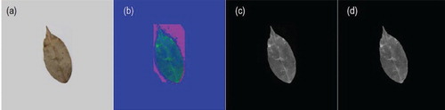
The leaf images contain only one object, the leaf. Since all leaves are not perfectly flat, image capturing would always cast a shadow underneath the leaf. The shadow would disrupt the edge detection as it has a huge contrast with the background, confusing the algorithms to draw the boundary based on shadow instead of on the leaf. Thus, it should be removed before image segmentation. Firstly, the image RGB value was changed to HSV value. Then, the channel with the most clear contrast between object and shadow was selected and used to identify the object boundary. As HSV value conversion alters the original color, this step serves as a guidance for the subsequent edge detection of RGB value leaf images, rather than producing a final image for feature extraction (Figure 1).

Figure 1. Shadow removing pre-processing. Thin streak of shadow can still be seen in (c), which is then removed in (d).

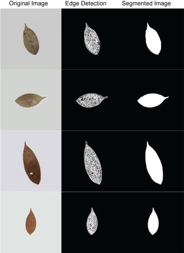
Subsequent processing involved a step in converting original images to grayscale images. The frequency of occurrence of the pixel intensities was inferred by the histogram and mapped to a uniform distribution. This step was performed to improve the appearance of images in terms of image contrast. Subsequently, images were converted from grayscale to binary images. Median filter (size 3 × 3) was used to reduce image noise. Image segmentation was performed to isolate the leaf object on images. The Canny edge detector algorithm, which is a powerful edge detector, is used to detect the edge of the leaf (Canny 1986). Any color patches, ID marking and small holes were removed by applying binary gradient mask on leaf images to stretch the leaf contents using the vertical structuring element followed by the horizontal structuring element to fill in the interior gaps inside leaves image. The latter was performed to remove the components inside the leaf image for the segmentation process. Then, the leave object boundaries were extracted by removing any deformity within the leaf outline and displayed the complete leaf in white patch. Figure 2 shows some leaf images and their respective processed images. The binary images removed any deformity within the leaf outline and displayed the complete leaf in white patch.

Figure 2. Image segmentation process.

Feature extraction

Processed images from previous steps were transformed into a set of parameters that describe the leaf features. There are four classes of features extracted in this study: morphological features (shape), Hu moment invariants feature, texture features and histogram of oriented gradients. These features were selected specifically to obtain the important properties for image leaves, and to obtain the numeric values that can be used to distinguish between the different types of image leaves. Several feature methods, as described below were implemented to improve the accuracy of detection and matching criteria.

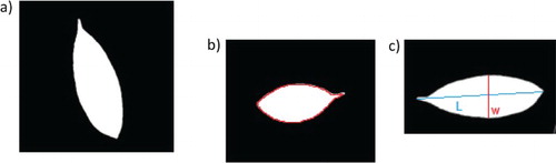
Shape features are a set of features commonly used in many studies. Shape values included in this study are: area, perimeter, eccentricity, and minor and major axes as shown in Figure 3. The efficiency of these features is proven in the algae classification study by Mosleh et al. (2012).

Figure 3. Selected shape features. (a) Area, (b) perimeter and (c) major and minor axes.

Hu moment invariants are seven moment features that can be used to describe shapes and these are invariants to rotation, translation and scaling. These invariants are extracted as described in the similar previous work (Hu 1962). Central moments and center of mass of the images were calculated, followed by Hu moments and saved in a vector as an output.

Leaf texture is a common feature used in many studies (Kebapci et al. 2010). The texture features were extracted using the Gray Level Co-occurrence Matrix analysis (Ramos and Fernández 2009; Zhang et al. 2012) and this was performed using the texture analysis toolbox from Matlab (MathWorks 2001). The gray-level co-occurrence matrix reveals important properties about the spatial distribution of the gray levels in the leaf texture image. Contrast level, correlation, energy and homogeneity are used mainly to produce the co-occurrence matrix which represented the leaf texture image using 8 bit for gray scale level * 4 levels * 2 values for each level = 64 feature values.

Histogram of oriented gradients (HOG) is a feature descriptor used in computer vision and image processing. The generation of this feature is adopted from the work of Junior et al. (2009). The steps involved are gradient computation, orientation binning, descriptor blocks and block normalization. The HOG vector size is 80 because we have 4 overlapping blocks in the image, each of size 2 × 2 cells, where each block gave us 4 histograms of oriented gradients, each containing 5 bins. Thus, the number of HOG features is 4 × 4 × 5 = 80. The features extracted to represent the input vectors are shown in Table 1.

Table 1. Features extracted for input vectors.

Features	No.
Shape features	5
Area, perimeter, eccentricity, minor axis, major axis
Moment features	9
Moment invariants
Central moments
Center of mass
Co-occurrence matrix	64
Histogram of oriented gradients	80
Total number of features	158

Classification models training

Two machine learning classification algorithms, ANN and SVM, were implemented. Data samples were divided into training and testing sets. Twenty images per species were used to build the training dataset, totaling to 60 images and the remaining samples were used for testing the dataset.

The ANN was developed using a multilayer perceptron network to train and classify the extracted features values into three classes representing the three species used in this study. The architecture of the ANN is a three-layer feed-forward network. More hidden layers could enhance the classification process; however it would take more iterations of training the data, which will lead to a higher risk of overfitting (Markovic et al. 1997). Hence, considering the limited dataset used in this study, only one hidden layer was used. The architecture of ANN consists of 158 input nodes, 10 hidden nodes and three output nodes. The 158 input nodes refer to the number of features, while three output nodes refer to the 3 species we classified. The default setting of the number of hidden nodes in the Matlab Neural Network Toolbox setting is 10, as this setting generally produces good results. Thus, the default setting of 10 hidden nodes was applied in this study. These neurons and the network were trained with the scaled conjugate gradient back-propagation algorithm (Møller 1993).

Sample images were divided into three blocks: 70% for training, 10% for validation and 20% for testing. As shown in Table 2, a total of 60 data samples were classified into two sets, training and testing datasets. Twelve samples were used for training purpose which represents 20% of total samples for both ANN and SVM algorithms. Forty-two samples were used for testing in the ANN algorithm which represents 70% of total samples, and 48 samples were used for testing in the SVM algorithm which represents 80% of the total sample. In ANN, six samples were selected randomly for validation purposes which represent 10% of total samples. Table 2 presents specimen allocation used for training and testing for ANN and SVM model development. The distribution of the specimen was done randomly to avoid biasness.

Table 2. Sample allocation of both machine learning algorithms.

Model algorithm	ANN	SVM
Training	42 (70%)	48 (80%)
Validation	6 (10%)	–
Testing	12 (20%)	12 (20%)
Total	60 (100%)	60 (100%)

The data from the training set were used for network training; the validation set for measuring network generalization to prevent overfitting and the testing set for measuring network performance after training. The number of epochs varies in different runs, typically ranging from 20 to 50, as it is determined by MATLAB Neural Network Toolbox. Using the validation set, the system checks the generalization ability of the network in every iteration. Once the ability starts to reduce, the training of ANN stops and the trained ANN will then be used for predicting testing set.

SVM was implemented using the R package software. The Kernel-based Machine Learning Lab (Kernlab) package was used to develop the SVM model (Zeileis et al. 2004). It is an extensible package for kernel-based machine learning methods in R, and contains several types of kernels that can be implemented in SVM. We used the radial basis function kernel in our study as it has demonstrated good results in other studies (Sarimveis et al. 2006; Kiranyaz et al. 2010). The parameters used in training SVM were sigma (σ = 0.01) and cost (C = 3). Both parameters were optimized by trial-and-error and the results are available at https://data.mendeley.com/datasets/tvw4gy5ywy/draft?a=c0f5490b-cf62-4c4d-9908-06dd2f803ee8.

In SVM, the images are divided into two blocks: 80% for training and 20% for testing (Table 2). Kernlab packages automatically assign data from testing set for validation, thus user input for validation set was not required. The data from training set were used for network training and cross validation, while the testing set data were used for measuring network performance.

Model performance and comparison criteria

Two models have been trained using the same data. Performance of these two models was then evaluated and compared using three adopted criteria: accuracy, receiver operating characteristics (ROC) and area under curve (AUC). The confusion matrix was constructed to display the predicted results compared with labeled classes. Accuracy indicates the percentage of the values that show true and consistent results. It can be derived from the confusion matrix and is defined as the formula below: where TP indicates true positive, TN indicates true negative, FP indicates false positive and FN indicates false negative.

The ROC value indicates the performance of a binary classifier system as its discrimination threshold is varied. It is a graphical plot of sensitivity or true positive rate versus false positive rate. The plot is then used to calculate AUC using the trapezoidal rule. Threshold values of AUC are adopted from the study of Mingyang et al. (2008). AUC ranges from 0 to 1, where a score of >0.9 indicates outstanding discrimination, a score between 0.8 and 0.9 is excellent, and a score >0.7 is acceptable.

Results

Both machine learning algorithms, ANN and SVM, were used to train the identification models and were tested with 20% of the image samples. The prediction results are shown in confusion matrices (Table 3(a) and (b)). Both models achieved same results, accurately identifying 10 out of 12 tested samples. Both models correctly identified all specimens of F. pellucidopunctata, but misclassified one specimen each of F. benjamina and F. sumatrana, respectively.

Table 3. Classification results of (a) artificial neural network model and (b) support vector machine.

(a)	Actual	Ficus benjamina	Ficus pellucidopunctata	Ficus sumatrana	(b)	Actual	Ficus benjamina	Ficus pellucidopunctata	Ficus sumatrana
	Predicted					Predicted
	Ficus benjamina	3 (75.0%)	0	1 (25.0%)		Ficus benjamina	3 (75.0%)	0	1 (25.0%)
	Ficus pellucidopunctata	0	4 (100%)	0		Ficus pellucidopunctata	1 (25.0%)	4 (100%)	0
	Ficus sumatrana	1 (25.0%)	0	3 (75.0%)		Ficus sumatrana	0	0	3 (75.0%)

Note: Outputs of models (rows) were compared with the target species (columns).

The ROC for both models were plotted as shown in Figure 4. Both plots are hard to compare just by subjective human vision. Thus, the AUC was calculated and recorded in Table 4. Overall, both models achieved similar results. The accuracy of both models is the same (83.3%), but the AUC values are different. The ANN model had a higher value in identifying F. benjamina and F. pellucidopunctata, while the SVM model had a higher value in identifying F. sumatrana. Overall, the ANN model performed slightly better than the SVM model with a total AUC difference of 0.1562.

Figure 4. The receiver operating characteristics (ROC) curve of both models.

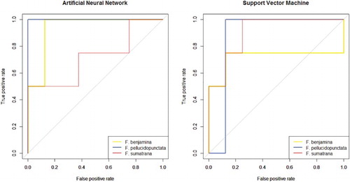
Table 4. Accuracy and area under curve (AUC) comparison of both models.

		Area under curve (AUC)
Models	Accuracy	F. benjamina	F. pellucidopunctata	F. sumatrana	Total
Artificial neural network	83.3%	0.9375	1.0000	0.7188	2.6563
Support vector machine	83.3%	0.7188	0.8750	0.9063	2.5001
Difference	0	0.2187	0.1250	−0.1875	0.1562

Discussion

Two models were trained using ANN and SVM, respectively, and their performances were compared. Both models achieved the same accuracy (83.3%). In order to further validate the performance of these models, we used ROC and AUC measures. The ROC curve is a helpful tool for choosing a threshold that appropriately maximizes the trade-off between sensitivity and specificity and the quantitative assessment of the model. The ANN model had a higher AUC value than the SVM model; and with additional comparison of AUC, we found that performance of the ANN model is slightly better than the SVM model. These results are consistent with the study of Gutiérrez et al. (2015) where the ANN model performed slightly better than the SVM model in identifying grapevine varieties. This can be taken as an indication that these models can be utilized for these kinds of tasks.

When large datasets are infeasible to achieve due to many reasons, experiments end up with smaller datasets. The neural network, an excellent tool under large sample conditions, has low performance when it comes to smaller datasets. In this work, overfitting was a concern when developing the ANN classifier model. In the work of Mao et al. (2006), ANN accuracy was lower than 50% when their training data was small (n < 14). As the training datasets increased to 40, the accuracy levels increased to 67.5%. In this study, we employed 42 training datasets and used only one hidden layer to construct ANN. Low complexity of ANN architecture shows more robustness to the underlying distributions of data (Markovic et al. 1997). Besides, another classifier build by SVM shows similar results with the ANN classifier. For further confirmation, we performed leave-one-out cross validation on ANN models. The misclassification rate was 0.217, which does not deviate much from the accuracy achieved. Thus, the ANN classifier developed is believed to have been avoided from overfitting.

Herbaria around the world contain a vast number of specimens and are a good source of information for traditional botanists. This study explored the potential use of specimens in a herbarium to accelerate the identification process via the machine learning approach. A similar study was done by Clark et al. (2012) using the ANN approach to identify four Tilia species with herbarium leaf images achieved a 44% accuracy. Our study achieved an 83.3% accuracy, significantly higher perhaps due to the quality of the datasets that were fed into the identification models. Clark et al. (2012) employed an automated technique to extract leaf images, which is a more difficult task than species identification. However, the automated extraction system poses risks in increasing the noise in input data, which explains the low accuracy achieved. In this study, we focused on the task of species identification with the aim to determine the feasibility of using pattern recognition techniques. Thus, we manually selected leaves that are not damaged with intact shape outlines. Though slow, manual selection arguably results in better data quality.

We believe that a higher accuracy can be achieved if more features such as color, shape and texture can be extracted and used as demonstrated by Kebapci et al. (2010). There are many other studies aiming to automate plant species identification. However, it is difficult to directly compare results with other studies as there are interspecies variations of leaf shapes, differences of leaf shape across habitats, sampling efforts, the availability of software and datasets diverse (Hearn 2009). The Leafsnap system developed was able to identify plant species of North America at 96.8% accuracy (Kumar et al. 2012). This system does not have information about tropical plant species, and only recognizes one species in Ficus genus. The system takes leaf image as the input and generates a list of match species. Their study used species match rank as the performance metric and declared that a species is correctly matched if it falls within the top five results. Thus, it is hard to directly compare the performance of the study done by Kumar et al. (2012) with the accuracy achieved in our study. Nevertheless, reasonable accuracy was achieved in this study.

Manual plant identification by taxonomists involves examining many parts of a plant including their leaves before a reliable decision can be made to identity a species. Taxonomic keys are used in the identification process along with comparative assessments with herbarium samples. The system developed in this work extracted only the leaf character and achieved 83.3% accuracy, which can be regarded as a reasonable result. It is important to note that these automated systems would perhaps never achieve the accuracy levels of taxonomists but it is a good platform of converting taxonomists’ knowledge into an application, which can be used by people without taxonomical background, especially with the scarcity of expertise in the field of taxonomy these days. This model lays a platform where a rapid method for assisting scientists to identify Ficus species when the expertise resource is nowhere accessible. Future studies will test the robustness of the model by including more species as well as by improving the selection of features used.

Conclusion

In this study, we have presented baseline automated identification techniques of three Ficus species based on herbarium leaf images, using the pattern recognition approach. Two machine learning algorithms: ANN and SVM have been used to build identification models. Both models achieved satisfactory results demonstrating their usefulness in identification tasks. The study presented here showed that automated classification of selected Ficus species that had similar leaf shapes is feasible based on leaf images. Though the developed system is not intended to replace human taxonomists, it may provide a rapid and easily accessible technique to identify plants with acceptable accuracy. We chose to work on species of Ficus as it is a large genus and species identification can be difficult especially to non-taxonomists. In future, the robustness of the system could be improved by including more species of Ficus.

Acknowledgements

The authors appreciate the cooperation from the University of Malaya Herbarium, housed by Rimba Ilmu Botanic Garden, in providing specimens for image capturing. The University of Malaya is acknowledged for providing research facilities.

Disclosure statement

No potential conflict of interest was reported by the authors.

Additional information

Funding

This work was supported by the University of Malaya [grant number Living Lab LL023-16SUS], [grant number Living Lab (LLO20-16SUS)].

References

- Abu A, Lim LHS, Sidhu AS, Dhillon SK. 2013a. Biodiversity image retrieval framework for monogeneans. Syst Biodivers. 11(1):19–33. doi: 10.1080/14772000.2012.761655
- Abu A, Lim LHS, Sidhu AS, Dhillon SK. 2013b. Semantic representation of monogenean haptoral bar image annotation. BMC Bioinf. 14(1): 48. doi: 10.1186/1471-2105-14-48
- Berg CC, Corner EJH, Jarrett FM. 2006. Moraceae-genera other than Ficus: Flora Malesiana-Series 1. Spermatophyta. 17(1):1–146.
- Boser BE, Guyon IM, Vapnik VN. 1992. A training algorithm for optimal margin classifiers. In: Haussler D, editor. 5th annual ACM workshop on COLT. Pittsburgh (PA): ACM Press; p. 144–152.
- Canny J. 1986. A computational approach to edge detection. IEEE Trans Pattern Anal Mach Intell. PAMI-8:679–698. doi: 10.1109/TPAMI.1986.4767851
- Chapelle O, Haffner P, Vapnik VN. 1999. Support vector machines for histogram-based image classification. IEEE Trans Neural Netw. 10:1055–1064. doi: 10.1109/72.788646
- Clark JY, Corney DP, Tang HL. 2012. Automated plant identification using artificial neural networks. CIBCB 2012. Proceedings of the IEEE Symposium on Computational Intelligence in Bioinformatics and Computational Biology; May 9–12; San Diego, CA: IEEE. doi: 10.1109/CIBCB.2012.6217215
- Coltelli P, Barsanti L, Evangelista V, Frassanito AM, Gualtieri P. 2014. Water monitoring: automated and real time identification and classification of algae using digital microscopy. Environ Sci Process Impacts. 16:2656–2665. doi: 10.1039/C4EM00451E
- Cook JM, Rasplus J-Y. 2003. Mutualists with attitude: coevolving fig wasps and figs. Trends Ecol Evol. 18:241–248. doi: 10.1016/S0169-5347(03)00062-4
- Gutiérrez S, Tardaguila J, Fernández-Novales J, Diago MP. 2015. Support vector machine and artificial neural network models for the classification of grapevine varieties using a portable NIR spectrophotometer. PLoS One. 10:e0143197. doi: 10.1371/journal.pone.0143197
- Hearn DJ. 2009. Shape analysis for the automated identification of plants from images of leaves. Taxon. 58:934–954.
- Hu J, Li D, Duan Q, Han Y, Chen G, Si X. 2012. Fish species classification by color, texture and multi-class support vector machine using computer vision. Comput Electron Agric. 88:133–140. doi: 10.1016/j.compag.2012.07.008
- Hu M-K. 1962. Visual pattern recognition by moment invariants. IRE Trans Inf Theory. 8:179–187.
- Junior OL, Delgado D, Gonçalves V, Nunes U. 2009. Trainable classifier-fusion schemes: An application to pedestrian detection. Proceedings of the Intelligent Transportation Systems, 2009 ITSC’09 12th International IEEE Conference. St. Louis: IEEE.
- Kalafi EY, Tan WB, Town C, Dhillon SK. 2016. Automated identification of monogeneans using digital image processing and K-nearest neighbour approaches. BMC Bioinf. 17:511. doi: 10.1186/s12859-016-1376-z
- Kalafi EY, Town C, Dhillon SK. 2017. How automated image analysis techniques help scientists in species identification and classification? Folia Morphol. doi:10.5603/FM.a2017.0079.
- Kebapci H, Yanikoglu B, Unal G. 2010. Plant image retrieval using color, shape and texture features. Comput J 54(9):1475–1490. doi: 10.1093/comjnl/bxq037
- Kiranyaz S, Gabbouj M, Pulkkinen J, Ince T, Meissner K. 2010. Classification and retrieval on macroinvertebrate image databases using evolutionary RBF neural networks. Proceedings of the Proceedings of the International Workshop on Advanced Image Technology, Kuala Lumpur, Malaysia.
- Kumar N, Belhumeur PN, Biswas A, Jacobs DW, Kress WJ, Lopez IC, Soares JV. 2012. Leafsnap: A computer vision system for automatic plant species identification. In: Computer vision–ECCV 2012. Berlin: Springer. p. 502–516.
- Lambert FR, Marshall AG. 1991. Keystone characteristics of bird-dispersed Ficus in a Malaysian lowland rain forest. J Ecol. 79:793–809. doi: 10.2307/2260668
- Leow LK, Chew L-L, Chong VC, Dhillon SK. 2015. Automated identification of copepods using digital image processing and artificial neural network. BMC Bioinf. 16(18):S4. doi: 10.1186/1471-2105-16-S18-S4
- Mao R, Zhu H, Zhang L, Chen A. 2006. A new method to assist small data set neural network learning. ISDA’06. Proceedings of the Sixth International Conference on Intelligent Systems Design and Applications; October 16–18; Jinan: IEEE. Vol. 1, p. 17–22.
- Markovic M, Milosavljevic M, Samcovic A. 1997. A performance analysis of the multilayer perceptron in limited training data set conditions. 1997. Proceedings of the 13th International Conference on Digital Signal Processing, DSP 97, July 2–4; Santorini, Greece: IEEE.
- MathWorks. 2001. Image processing toolbox. http://cis-linux1.temple.edu/∼latecki/Courses/CIS581-02/MatCIS581-02/Matlab_images_tb.pdf
- Mingyang L, Yunwei J, Kumar S, Stohlgren TJ. 2008. Modeling potential habitats for alien species dreissena polymorpha in continental USA. Acta Ecol Sin. 28:4253–4258. doi: 10.1016/S1872-2032(08)60080-3
- Møller MF. 1993. A scaled conjugate gradient algorithm for fast supervised learning. Neural Netw. 6 (4):525–533. doi: 10.1016/S0893-6080(05)80056-5
- Morwenna S, Marsham S, Chang CW, Chong VC, Sasekumar A, Sarinder KD, Loh KH. 2016. The use of otolith morphometrics in determining the size and species identification of eight mullets (Mugiliformes: Mugilidae) from Malaysia. Sains Malays. 45 (5):735–743.
- Mosleh MA, Manssor H, Malek S, Milow P, Salleh A. 2012. A preliminary study on automated freshwater algae recognition and classification system. BMC Bioinf. 13:S25. doi: 10.1186/1471-2105-13-25
- Ramos E, Fernández DS. 2009. Classification of leaf epidermis microphotographs using texture features. Ecol Inform. 4:177–181. doi: 10.1016/j.ecoinf.2009.06.003
- Salimi N, Loh KH, Dhillon SK, Chong VC. 2016. Fully-automated identification of fish species based on otolith contour: using short-time Fourier transform and discriminant analysis (STFT-DA). PeerJ. 4:e1664. doi: 10.7717/peerj.1664
- Sarimveis H, Doganis P, Alexandridis A. 2006. A classification technique based on radial basis function neural networks. Adv Eng Softw. 37 (4):218–221. doi: 10.1016/j.advengsoft.2005.07.005
- Schneider CA, Rasband WS, Eliceiri KW. 2012. NIH image to ImageJ: 25 years of image analysis. Nature Met. 9 (7):671–675. doi: 10.1038/nmeth.2089
- Shanahan M, So S, Compton SG, Corlett R. 2001, November. Fig-eating by vertebrate frugivores: a global review. Biol Rev. 76:529–572. doi: 10.1017/S1464793101005760
- Wang J, Lin C, Ji L, Liang A. 2012. A new automatic identification system of insect images at the order level. Knowl Based Syst. 33:102–110. doi: 10.1016/j.knosys.2012.03.014
- Wong JY, Chu C, Chong VC, Dhillon SK, Loh KH. 2016. Automated otolith image classification with multiple views: an evaluation on sciaenidae. J Fish Biol. 89:1324–1344. doi:doi: 10.1111/jfb.13039.
- Zeileis A, Hornik K, Smola A, Karatzoglou A. 2004. Kernlab-an S4 package for kernel methods in R. J Stat Softw. 11:1–20. doi: 10.18637/jss.v011.i10
- Zhang H, Yanne P, Liang S. 2012. Plant species classification using leaf shape and texture. ICICEE. Proceedings of the International Conference on Industrial Control and Electronics Engineering; August 23–25; Xi’an: IEEE Computer Society. p. 2025–2028.