Assessing land use and land cover of the Marikina sub-watershed, Philippines

Abstract

The integrated remote sensing (RS) and geographic information system (GIS) approach was utilized in this study to classify land use and land cover (LULC), detect changes based over time, and identify transition trends in the Marikina sub-watershed, Laguna de Bay watershed, Philippines. Landsat 5 Thematic Mapper (TM) imageries acquired in 1999 and 2006 were pre-processed and classified using a supervised classification technique with maximum likelihood classifier algorithm in RS and were used to develop maps of the sub-watershed and sub-subwatershed levels in a GIS platform. LULC change analysis revealed that, from 1999 to 2006, significant changes occurred in the sub-watershed as indicated by the increase of agricultural (11.76%) and orchard (4.52%) areas at the expense of brushland (16.56%) areas. Other LULC such as water bodies, built-up, forest, and grassland remain almost unchanged. In the sub-subwatershed level, Tayabasan experienced minimal change, whilst Tanay had the most transitions. Overall accuracy and kappa statistics were then derived using the confusion matrix, which resulted in 96.15% and 95.49% for 1999 imagery, and 93.82% and 92.73% for 2006 imagery, respectively. LULC persistence and transition trends were analyzed using land change modeler, while the Markov chain model has been utilized to predict the LULC distribution in 2020 pertinent to rates of change from 1999 to 2006. This study contributes not only to the understanding of the past and present landscape of the sub-watershed, but also provides an idea of the areas that need rehabilitation for the formulation of suitable mitigation measures and strategies toward the sustainable management of the sub-watershed.

Keywords:

• confusion matrix
• land use/land cover persistence
• Markov chain
• maximum likelihood classifier
• transition trend

Introduction

Humans predominantly define the changes that are taking place on the Earth's terrestrial surface. In order to grasp the influence of man's utilization of natural resource base over time, which is often undocumented on the ground, the images generated by viewing the Earth from space provide the most accurate evidence. Over recent decades, Earth sensing satellite data have served as fundamental inputs in mapping features and structural developments, managing natural resources, and studying environmental changes (Park et al. 2011; Santillan et al. 2011; Torahi and Rai 2011; Ohri and Poonam 2012, Mallupattu and Reddy 2013).

The integration of remote sensing (RS) and geographic information system (GIS) has been used extensively in different parts of the world to further enhance the accuracy and timely information describing the landscape dynamics and extent of natural resources and their changes over time (Dong et al. 2009; Santillan et al. 2011, Liu et al. 2014; Mallupattu and Reddy 2013; Yagoub and Al Bizreh 2014). The most prominent application of integrated RS-GIS modeling is for vegetation mapping, which contributes to the analysis of land use and land cover (LULC) changes and transition trends. LULC change over time in response to the evolving economic, social, and biophysical conditions. The changes in LULC have become a pivotal component of the strategies for managing natural resources and monitoring environmental changes (Ohri and Poonam 2012). The impacts of LULC change have also become increasingly important in light of carbon dynamics, climate change, hydrology, and biodiversity (Sohl and Sleeter 2012). Detecting past changes, and predicting these kinds of changes in the future, play a key role in decision making and long term planning. One of the most functional models in predicting the LULC dynamics several periods into the future is the Markov chain stochastic model. Several studies used Markov chain with the assumption that the LULC transition probability indicates the likelihood of changing from one class to another within two discrete times (Mubea et al. 2010; Behera et al. 2012; Yagoub and Al Bizreh 2014).

In the Philippines, significant progress has been made in analyzing LULC change in different watersheds and regions in the country using various models, including RS and GIS (Verburg et al. 2006; Overmars et al. 2007; Combalicer et al. 2011; Estoque and Murayama 2011; Santillan et al. 2011) to capture the drivers, patterns, and potential impacts of landscape changes. Amongst the watersheds in the country, Laguna de Bay watershed, with an area of about 3820 km², has been significantly altered owing primarily to anthropogenic activities (Nauta et al. 2003). With approximately 100 rivers and streams traversing the basin that are the source of fresh water recharge of the country's largest lake (Hernandez et al. 2012), this is considered as one of the country's vital watersheds. The Marikina sub-watershed, being the largest yet the most critical among the sub-watersheds of the Laguna de Bay watershed, is attributed to the shoaling in the western bay of the lake. It is conceptualized that the sedimentation is directly related to land conversion practices within the sub-watershed that have resulted in high erosion rates leading to greater pollution of the lake (Blanco and Nadaoka 2006). In the Laguna de Bay watershed, previous studies were undertaken utilizing RS and GIS separately in conjunction with other models. However, the integration of RS and GIS for classifying LULC, detecting changes over time, and identifying persistence and transition trends are yet to be fully explored. Therefore, this study seeks to utilize the integrated RS and GIS approach in mapping, to analyze the changes and trends on the past and present LULC conditions in the Marikina sub-watershed using Landsat Thematic Mapper (TM) imageries. Moreover, this study also aims to project LULC distribution in year 2020 using a Markov-based model.

Study area

The Marikina sub-watershed is one of the 24 hydrological sub-watersheds comprising the entire Laguna de Bay watershed located about 20 km east of Manila, Philippines (Figure 1). The geographical boundary of the sub-watershed lies between latitude 14°33′26.14″–14°50′11.91″ N and longitude 121°3′39.37″–121°19′32.45″ E. It has a drainage area of approximately 538 km² encompassing four cities and three municipalities. The highest elevation is the Mt. Irid (1469 m above sea level) which borders the northeastern side of the sub-watershed. The study area comprises of varied LULC including agricultural land, brushland, plantation, built-up, forest land, grassland, and water. A large extent of forest cover is found in the uplands at the northeast portion of the sub-watershed, while built-up areas are dominant on the western lowlands. Some portions within the sub-watershed may seem barren but are actually grasslands or arable lands depending on the seasonal condition that influence the crop rotating system specifically for the arable areas, where lands were tilled for crop production and then left to recover for a certain period. The sub-watershed is under two climatic types based on the Modified Corona Climate Classification System: Type I, on the western side with two pronounced seasons, is relatively dry from November to April and wet during the rest of the year; and Type III, on the eastern portion with no pronounced maximum rain period, has a short dry season lasting from 1 to 3 months. Based on the data of the Philippine Atmospheric, Geophysical and Astronomical Services Administration (PAGASA) from 1999–2006, the annual average temperature was 27.8°C, while the annual average precipitation was 2718 mm, normally peaking in the month of July. According to the census (National Statistics Office 2007), an average demographic growth rate of 3.99% was recorded between 2000 and 2007 in the municipalities and cities within the sub-watershed.

Figure 1. Location map of Marikina sub-watershed and its sub-subwatersheds (a) in the Laguna de Bay watershed (b), Luzon Island, Philippines (c).

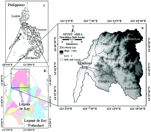
The digital elevation model (DEM) used for the sub-watershed delineation was extracted from the ASTER Global DEM through the online data pool at the USGS-NASA Land Processes Distributed Active Archive Center (https://lpdaac.usgs.gov/data_access). The sub-watershed delineation was carried out through a series of steps collectively known as terrain processing using HEC-GeoHMS (Hydrologic Engineering Center's Geospatial Hydrologic Modeling Extension) and the Arc Hydro tool in ArcGIS 10. The catchment extractions delineated more than 200 sub-subwatersheds, merged into eight sub-subwatersheds comprising the entire Marikina sub-watershed. These sub-subwatershed were further grouped into upper and lower Marikina sub-river basins (Figure 1). The upper Marikina sub-river basin covers Bosoboso, Tayabasan, Montalban, and Wawa sub-subwatersheds; while the lower Marikina sub-river basin encompasses Tanay, Marikina, Mango, and Nangka sub-subwatersheds.

Methodology

Image pre-processing

In this study, two Landsat 5 TM imageries covering the study area acquired on 13 November 1999 and 02 December 2006 (path 116, row 50), with pixel resolution of 30 m × 30 m, were obtained from USGS-EROS Global Visualization Viewer website (http://glovis.usgs.gov/) for LULC mapping. The selection of the data was dependent on the availability of satellite imageries in the USGS website that possess similar months in order to minimize the possible occurrence of change in land cover condition attributed to differences in atmospheric and weather conditions. The study area was extracted from the acquired satellite imageries using the generated sub-watershed boundary. The imageries were previously geometrically corrected to a level-one terrain (L1T), thus, already orthorectified to a universal transverse Mercator (UTM) projection zone 51 N-datum World Geodetic System (WGS) 1984. To minimize the effects caused by using time-series of satellite data collected in different dates and with different sun angles (Jensen 1996), the imageries were radiometrically corrected to at-sensor radiance. A standard atmospheric correction using dark-object subtraction using band minimum was also undertaken. Consequently, using the radiometrically and atmospherically corrected imageries, normalized difference vegetation index (NDVI) imageries were derived to refine the classification.

Image classification

Training

A modified classification scheme was based on the LULC classification scheme defined by Anderson et al. (1976) for interpretation of RS data at different scales and resolutions. The modified LULCs include forest, orchard, grassland, built-up areas, brushland, agricultural land, and water bodies. Forest land is classified as a parcel of land having a tree-crown areal density of 10% or more, and stacked with trees capable of producing timber or other wood products. Orchards are areas with fruit-bearing tree plantations, brushlands are areas characterized by vegetation dominated by brushes and shrubs, while agricultural land represents portions cultivated for annual cash crops. Grassland is defined as areas where natural vegetation is predominantly grasses and/or grass-like plants, while built-up areas are those of intensive use with much of the land covered by structures. Since there were some clouds and cloud shadows in the acquired remote satellite imageries, all potential clouds and cloud shadows were identified. Some of the clouds and cloud shadows detected in the southwestern portion of the sub-watershed are mainly developed areas. Therefore, these cloud and cloud shadow classes were combined with the built-up category. Field surveys were carried out to collect data for training and validating LULC interpretation from the satellite imagery of 2006, and for qualitative description of the characteristics of each LULC. Additionally, ancillary and historical data necessary for classification of 1999 imagery were also collected. Given that the study area is too dangerous and too remote for direct access due to steep slopes and the lack of roads or pathways, 70 random ground control points that represent each class were collected using a global positioning system (GPS) receiver incorporated with photo documentation to provide digital visualization of the area being studied.

Allocation

For the image classification, supervised classification technique with maximum likelihood classifier (MLC) algorithm was used. MLC is regarded as one of the most functional classifiers as it does not always necessitate large training datasets and its performance is comparable to other algorithms when size and location of the training samples are limited and of good quality (Václavík and Rogan 2009). However, this algorithm assumes that the statistics for each class in each band are normally distributed and calculates the probability that a given pixel belongs to a specific class. A total of 20 representative samples for each class were collected for the 1999 and 2006 imageries. Selection of training samples was done by incorporating imagery from Google Earth taken on 05 April 2006, in addition to the ground control points and ancillary data collected during the field surveys. It was also ensured that the separability of the classes measured using the Jeffries-Matusita Distance is ≥ 1.7 (Santillan et al. 2011), where value approaching 2.0 indicates satisfactory value for separability between the classes. For the post-classification, a 3 × 3 majority filter was applied to each imagery to smooth the salt-and-pepper appearance of the imageries by recoding isolated pixels classified differently from the majority class of the window (Lillesand et al. 2008). The classification maps were converted into a vector file and then to shapefile for further analysis.

Testing

Another independent set of samples of 90 polygons was randomly selected from each imagery for accuracy assessment. To assess the accuracy of the classified imageries, confusion matrices, also known as error matrices, which compare the relationship between the reference or ground-truth data and the corresponding results of an automated classification or the mapped data on a category-by-category basis (Congalton and Green 2008) were used. Overall, user's and producer's accuracies, and kappa statistics were then derived to quantify classification performance. The overall accuracy is the percentage of correctly predicted pixels, producer's accuracy is estimated from the percentage of correctly predicted pixels amongst the ground-truth pixels, while user's accuracy is the percentage of correctly predicted pixels amongst all predicted pixels (Shen et al. 2013). According to Torahi and Rai (2011), kappa statistics include the off-diagonal elements of the error matrices or the classification errors, and denotes agreement obtained after removing the proportion of agreement that could be expected to occur by chance. The kappa statistic or the KHAT statistic is computed as:(1) where r is the number of rows in the error matrix, x_ii is the number of observations in row i and column i, x_i+ and x_+i are the marginal totals of row i and column i, respectively, and N is the total number of observations included in the matrix (Lillesand et al. 2008).

Change detection

After the imageries’ classification, a post-classification comparison change detection algorithm was employed to discriminate the changes in LULC from 1999 to 2006. Based on the study of Jensen (2005), the latter algorithm is the most common approach to change detection as evidenced by several studies that resulted in successful LULC change monitoring worldwide. The change detection analysis provides “from-to” change information and the kind of landscape conversions that have occurred can be easily calculated and mapped (Torahi and Rai 2011). A change detection map with 81 combinations of “from-to” change information was derived for the 1999 and 2006 nine-class maps including clouds and cloud shadows.

Trends identification and change projection

In order to understand the nature and extent of LULC change based on gains and losses, persistence, and specific transitions between chosen categories, land change modeler (LCM) for ecological sustainability tool was used. This tool was applied to distinguish the locations and the extent of the major LULC changes and persistence using the classified LULC maps from 1999 and 2006 as inputs parameters. Moreover, the spatial trends of major transitions between LULC classes were estimated using the trend surface analysis (TSA). This spatial trend analysis tool provides interpretation through a best fit polynomial trend surface to address the underlying pattern of complex change (Eastman 2012). A sixth-order polynomial was used to facilitate visualization of the locations of major LULC transitions in the span of the study.

To estimate the probabilities of change in each LULC in the future, a Markov chain analysis model was used. According to Lambin (1994), given the difficulties in designing deterministic models of LULC change processes, it is convenient to consider them as stochastic where variable states are not described by unique value but rather by probability distributions. For LULC, the possibility that the system will be in a given state at a given time (t+1) may be derived from the knowledge of its state at any earlier time (t), and does not depend on the history of the system before time n_t, also known as first-order process (Bell 1974). The Markov process is an example of this stochastic process. Lambin (1994) stated that if the Markov process can be treated as a series of transitions between certain values or states, it is called a Markov chain. In the case of LULC change, the states of the system are determined as the amount of land occupied by various classes, measured as percentages of the area of each landscape unit. In order to model a process of LULC change by a Markov chain, the following mathematical equation derived by Lambin (1994) was used:(2) where n_t+1 is the output LULC proportion column vector, M is the m × m transition matrix for the time interval from t to t+1, and n_t is the input LULC proportion column vector. Using the 1999 and 2006 LULC maps as inputs, the Markov module was utilized to create transition probabilities and transition area matrices that project the LULC for year 2020. The transition probabilities illustrate the likelihood that a pixel of a given class will change to any other class or be retained in the next period, while the transition areas express the total area (in cells) that are expected to change in the next period (Eastman 2012).

Results and discussion

Classification map and change statistics

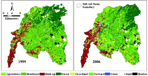
The classified LULC maps of the Marikina sub-watershed for 1999 and 2006 (Figure 2) illustrate a substantial change in the landscape of the study area. The results of the LULC distribution for years 1999 and 2006 revealed that brushland was the dominant LULC category (Table 1). However, based on the statistics generated, this category experienced the most significant reduction, by 16.56%, with respect to the total watershed area. Other LULCs that showed reduction in area include forest and grassland by 0.80% and 0.55%, respectively. The reduction in forest area supports the report of the main government environmental institution in the country which prompted the declaration of the portion of the sub-watershed as a protected area (Parinas and Paringit 2013). On the other hand, the analysis presented an increased in agriculture (11.76%), orchard (4.52%), water (1.98%), and built-up (1.32%) areas. Based on visual interpretation of the classification maps incorporating with the Google Earth imagery, a larger reduction in forest area is anticipated in view of the clouds and cloud shadows that covered the supposed forested areas specifically at the northeast (1999 imagery) portions of the sub-watershed.

Table 1. Summary of land use/land cover change statistics from 1999 to 2006 in the Marikina sub-watershed.

	1999		2006
Land use/cover class	Area (km^2)	%	Area (km^2)	%	% Change from 1999 with respect to total sub-watershed area
Water	2.70	0.50	13.34	2.48	1.98
Agriculture	27.87	5.18	91.10	16.94	11.76
Brushland	203.73	37.88	114.66	21.32	−16.56
Built-up	69.87	12.99	76.96	14.31	1.32
Forest	108.76	20.22	104.45	19.42	−0.80
Grassland	36.72	6.83	33.79	6.28	−0.55
Orchard	68.20	12.68	92.53	17.21	4.52
Cloud	14.17	2.63	6.27	1.17	−1.47
Shadow	5.82	1.08	4.72	0.88	−0.20

Negative value indicates decrease in area covered.

Figure 2. Land use/land cover maps of the Marikina sub-watershed derived from the analysis of the Landsat imageries: 1999 and 2006.

To aid in the interpretation of the changes occurred in the sub-watershed, a transition matrix (Table 2) was created based on the Markov chain (Lambin 1994). The transition matrix is comprised of the early year (1999) in the row axis with similar classes from the later year (2006) on the column axis. The matrix provides probabilities that reflect the statistics of the direction of LULC change. Interpretation of the values in the matrix shows that, although 43.36% of the brushland area in 1999 was retained as brushland in 2006, a large portion (22.34%) was transformed into agriculture in 2006. This may form part of the 16.56% reduction of brushland area on the study period which was probably caused by the rampant slash-and-burn farming by the inhabitants (Nicer 2004) to pave the way for the cultivation of annual cash crops for subsistence as evidenced by the 11.76% increase in agriculture (Table 1). In the case of forest, although 58.74% remains intact from 1999 to 2006, it still experienced denudation due to transformation into orchard (22.15%) category which may be due to the illegal logging that is persistent in the upper sub-subwatersheds where most of the forestlands are located (Nicer 2004; Parinas and Paringit 2013). The probable percentage of grasslands that were converted into agriculture (22.77%) and built-up (21.47%) areas in 2006 may be the reason for the reduction in area of the former of which only 19.60% remained unchanged. In the study period, 46.76% of the water body remained unchanged, while significant coverage (31.39%) was converted into built-up areas in 2006. The increase in built-up, agricultural, and plantation areas is a very good representation of demographic growth, similar to the reports of Lambin et al. (2003), Verburg et al. (2006), and Ohri and Poonam (2012). Classification error may be the reason for the drastic conversion of forest (1.53%) area into water, but the conversion from other LULCs is due to the overflow of the rivers and flood occurring in some places in the sub-watershed. A little more than 77% of the built-up areas were retained from 1999 to 2006, which can be explained by the fact that urbanized areas are highly resistant to LULC change (Fukushima et al. 2007). The relatively rare and unlikely conversions into agriculture, grassland, orchard, forest, and brushland areas with an equivalent total of 16.01%, are basically assumed as classification errors, which, in the case of forests, orchards, and brushlands may be attributed to the portions of the built-up associated pixels covered by tree canopies as they grow and expand (Torahi and Rai 2011; Hountondji et al. 2012). In Table 2, the main diagonal of the matrix provides the probability of the LULC that remained unchanged in the span of 7 years and are listed in descending order.

Table 2. Transition probability matrix of land use/land cover changes from 1999 to 2006 in the Marikina sub-watershed.

	2006
1999	Built-up	Forest	Agriculture	Water	Brushland	Orchard	Grassland	Cloud	Shadow
Built-up	0.7709	0.0061	0.0866	0.0564	0.0042	0.0095	0.0537	0.0043	0.0084
Forest	0.0112	0.5874	0.0382	0.0153	0.0949	0.2215	0.0158	0.0080	0.0078
Agriculture	0.0690	0.0233	0.5614	0.0203	0.0669	0.0339	0.1820	0.0201	0.0231
Water	0.3139	0.0173	0.0854	0.4676	0.0103	0.0067	0.0577	0.0324	0.0087
Brushland	0.0403	0.0435	0.2234	0.0102	0.4336	0.1741	0.0588	0.0101	0.0058
Orchard	0.0412	0.2552	0.1317	0.0399	0.0644	0.3889	0.0441	0.0238	0.0108
Grassland	0.2147	0.0966	0.2277	0.0227	0.1629	0.0613	0.1960	0.0107	0.0075
Cloud	0.0127	0.5428	0.0864	0.0073	0.1515	0.1118	0.0474	0.0167	0.0234
Shadow	0.0139	0.3222	0.1611	0.0320	0.2171	0.1713	0.0424	0.0245	0.0155

It can be observed that the largest areas of brush, orchard, and agricultural lands are located in the Bosoboso sub-subwatershed (Figure 3). Wide valley floodplain is prominent in this sub-subwatershed compared to other sub-subwatersheds. Based on the ancillary and historical data gathered during the field visits, brushlands and orchards located in this sub-subwatershed are interspersed with subsistence farming of rice, corn, sweet potato, and vegetable crops. Orchards typically consist of mango, jackfruit, citrus, cashew, and coconut. Built-up areas, on the other hand, dominated the Marikina sub-subwatershed which is situated in the urbanized portion of the sub-watershed. Thick vegetation consisting of old and secondary growth forest is observed in the Montalban sub-subwatershed. This is particularly located on the periphery of the steep mountains which serve as landmarks of this sub-subwatershed. Large portions of grassland are found in the Tanay and Marikina sub-subwatersheds. Grasslands are commonly interspersed with patches of brush and small trees. The lower Marikina sub-river basin experienced the largest conversions specifically on the brushland, orchard, forest, and agriculture classes, mainly because it is more accessible to people. For Mango, Nangka, Marikina, and Bosoboso sub-subwatersheds, decrease in brushland (31.01%, 27.14%, 22.93%, and 18.05%) and increase in agriculture classes (19.85%, 23.11%, 13.70%, and 12.94%), respectively, are apparent. The loss of forest resources (15.24%) and the increase in orchard areas (20.19%) are prominent in Tanay sub-subwatershed.

Figure 3. Land use/land cover distributions in the sub-subwatersheds within the Marikina sub-watershed derived from the analysis of the Landsat imageries: 1999 and 2006.

Change detection accuracy assessment

To measure the performance of the MLC algorithm, the confusion matrix was employed as summarized in Table 3. The 1999 and the 2006 LULC maps have overall accuracies of 96.15% and 93.82%, and kappa statistics of 95.49% and 92.73%, respectively. The producer's and user's accuracies of each LULC class were consistently high relative to the minimum level of interpretation accuracy of 85% for the identification of LULC classes from RS data according to Anderson (1971). In the 1999 LULC map, the producer's accuracy was the lowest for the grassland class (85.71%), as some of the lands dominated by grasses were misclassified as agricultural areas. The user's accuracy was the lowest for the orchard (69.70%) and brushland (82.64%), as some sites were identified as forest in the reference data. In the 2006 LULC map, the producer's accuracy was the lowest for the orchard category (58.33%), as some of the plantations were misclassified as forest. The user's accuracy was the lowest for the forest (81.33%) and brushland (81.82%), where some sites in these categories were identified as orchard. The expected overall change detection accuracy was also calculated by multiplying the individual classification accuracies (Torahi and Rai 2011), which resulted in 90.21%. The high percentage of accuracies acquired from the map classifications and change detections for 1999 and 2006 imageries are reflective of the rigorous classification algorithm described in detail in the Allocation section.

Table 3. Summary of classification accuracies (%) for 1999 and 2006 land use/land cover changes in the Marikina sub-watershed.

	1999		2006
Land use/cover class	Producer's	User's	Producer's	User's
Water	96.12	99.53	100.00	96.08
Agriculture	96.90	89.29	88.89	88.89
Brushland	91.54	82.64	93.10	81.82
Built-up	99.36	95.98	100.00	98.94
Forest	90.18	97.49	89.71	81.33
Grassland	85.71	95.80	100.00	100.00
Orchard	97.87	69.70	58.33	91.30
Cloud	99.81	100.00	100.00	100.00
Shadow	99.07	98.15	88.64	95.12
Overall accuracy	96.15		93.82
Kappa statistics	95.49		92.73

Change analysis and transition trends

The result of the evaluation of gross gains and losses for each LULC classes from 1999 to 2006 is depicted in Figure 4. Positive value indicates gain while negative value indicates loss. A bidirectional change in all classes except for the negligible loss in water (0.16%) was observed. Major changes include gains of agriculture (8.54%), orchard (7.47%), and water (1.37%), and loss of brushland (13.06%). Minimal increase in the area covered by built-up (2.62%) and minimal decreases in the extent of forest (5.08%) and grassland (3.35%) were depicted. In order to balance the gains and losses, agriculture and orchard classes had the net expansions, whereas brushland attributed the net reduction.

Figure 4. Gross gains and losses of every land use/land cover classes in the Marikina sub-watershed from 1999 to 2006.

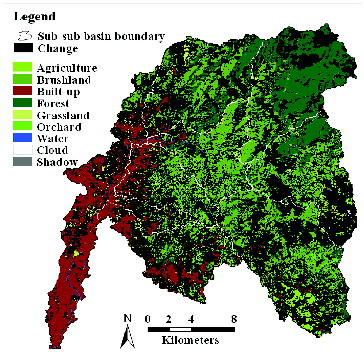
A cross-classification map (Figure 5) illustrates persistence or the areas where no change occurred, and the transition or the areas with depicted change in LULC classes in the span of the study. Based on the analysis, approximately 47.80% of the total area of Marikina sub-watershed remained unchanged from 1999 to 2006, while a larger proportion (52.20%) underwent conversion between the LULC categories. According to Rogan and Chen (2004), visual interpretation of the LULC transition and persistence map can be difficult if the locations of particular LULC changes are not clustered. This is true in the case of the study area where its landscape depends greatly on demographic migration and anthropogenic activities, thus, making the transition pattern complex and trends not easily deciphered.

Figure 5. Cross-classification map representing persistence (colour) and change (black) in land use/land cover classes in the Marikina sub-watershed between 1999 and 2006.

The TSA was employed to facilitate interpretation of the locations of complex transition patterns between LULC classes in the Marikina sub-watershed for a period of 7 years. Regarding the major conversions identified in the change analysis, four TSA maps (Figure 6) were created presenting the transitions from 1999 to 2006: brushland to agriculture; brushland to orchard; orchard to forest; and orchard to agriculture. Consequently, the maps illustrate a simulated surface that indicates the generalized locations of transition between LULC of interest specifically from unchanged to changed areas. The general trend of the main driving force for change in the landscape of the sub-watershed, from brushland to agriculture, was found on the western portion of the sub-watershed mainly on the Mango sub-subwatershed amidst the sloping terrain of the area varying from 3% to above 50%. The general location of land conversion from brushland to orchard was in the central part of the sub-watershed extending from steep slopes (30% to above 50%) of Wawa, Mango, and Bosoboso sub-subwatersheds. The major transition from orchard to forest generally occurred in the central toward the eastern part of the sub-watershed traversing Wawa, Bosoboso, and Tayabasan sub-subwatersheds with slopes ranging from 30% to 50%. Another substantial transition that contributed to the agricultural expansion in the sub-watershed from 1999 to 2006 at the expense of orchard was detected in the southern part of the study area, particularly at the Nangka sub-subwatershed with slopes ranging from 3% to 50%.

Figure 6. Trend surface analysis of major transitions between land use/land cover in the Marikina sub-watershed from 1999 to 2006: (a) brushland to agriculture; (b) brushland to orchard; (c) orchard to forest; (d) orchard to agriculture.

Markov prediction

The prediction of LULC patterns and distribution in year 2020 was carried out through Markov stochastic process with the assumption that the transition probability indicates the likelihood of changing from one class to another within two discrete times, which in this study refers to the years 1999 and 2006. It must be noted that the portions covered by clouds and cloud shadows in the 1999 and 2006 imageries were included in the projection of the 2020 LULC; thus, classification error pertinent to the actual cover is inevitable. The transition probability matrix (Table 4) shows the row categories which represent LULC classes in 2006 while column categories represent 2020 classes. Interpretation of the values in the matrix shows that the area with brushland has a 19.63% probability of being unchanged within a period of 14 years. On the other hand, there is a 27.85% chance that the brushland will be converted into agricultural land by 2020. In Table 4, unchanged pixels are along the major diagonal of the matrix.

Table 4. Transition probability matrix for prediction of land use/land cover in year 2020 by using land use/land cover maps of 1999 and 2006.

	2020
2006	Built-up	Forest	Agriculture	Water	Brushland	Orchard	Grassland	Cloud	Shadow
Built-up	0.5356	0.0305	0.1714	0.0924	0.0299	0.0271	0.0907	0.0101	0.0122
Forest	0.0433	0.3530	0.1129	0.0310	0.1321	0.2628	0.0408	0.0141	0.0100
Agriculture	0.1559	0.0823	0.3316	0.0352	0.1196	0.0736	0.1649	0.0183	0.0185
Water	0.4278	0.0527	0.1427	0.2045	0.0362	0.0271	0.0773	0.0209	0.0107
Brushland	0.0916	0.1124	0.2785	0.0264	0.1963	0.1741	0.0936	0.0155	0.0116
Orchard	0.0886	0.2891	0.1777	0.0473	0.1043	0.1966	0.0666	0.0180	0.0119
Grassland	0.2452	0.1157	0.2476	0.0383	0.1377	0.0998	0.0912	0.0128	0.0117
Cloud	0.0456	0.3780	0.1358	0.0222	0.1459	0.2023	0.0504	0.0101	0.0096
Shadow	0.0610	0.2696	0.1923	0.0347	0.1612	0.1899	0.0676	0.0144	0.0093

Based on the analysis of the LULC patterns and distribution per class (Table 5), by year 2020 agricultural lands (115.60 km², 4.55% increase) and built-up areas (93.29 km², 3.04% increase) will dominate the Marikina sub-watershed with a concomitant 9.06% decrease in brushland areas (65.95 km²) with respect to the total sub-watershed area, compared to the brushland-dominated sub-watershed in 1999 and 2006. It was observed that agricultural expansion and conversion to settlement areas are the main driving forces for change in the landscape of the sub-watershed. Furthermore, orchard and forested areas will decrease persistently by 2.28% and 1.84%, respectively. This may be an indication of the expected demographic increase in Marikina sub-watershed, which will bring pressure on the need for additional area to cultivate for basic subsistence as well as the incessant illegal logging activities within the sub-watershed. The summary of trends amongst LULC classes in the Marikina sub-watershed from 1999 to 2020 is further illustrated in Figure 7. The extent of LULC for the years 1999 and 2006 was classified from the Landsat imageries through the supervised classification technique with the MLC algorithm, while the 2020 coverage was projected using the Markov chain model. It can be observed from Figure 7 that drastic changes are being experienced by the sub-watershed, specifically in the agriculture, brushland, and built-up categories.

Table 5. Summary of land use/land cover change statistics from 2006 to 2020 in the Marikina sub-watershed.

	2006		2020
Land use/cover class	Area (km^2)	%	Area (km^2)	%	% Change from 2006 with respect to total sub-watershed area
Water	13.34	2.48	25.29	4.70	2.22
Agriculture	91.10	16.94	115.60	21.49	4.55
Brushland	114.66	21.32	65.95	12.26	−9.06
Built-up	76.96	14.31	93.29	17.35	3.04
Forest	104.45	19.42	94.57	17.58	−1.84
Grassland	33.79	6.28	47.91	8.91	2.63
Orchard	92.53	17.21	80.26	14.92	−2.28
Cloud	6.27	1.17	8.20	1.53	0.36
Shadow	4.72	0.88	6.74	1.25	0.38

Negative value indicates decrease in area covered.

Figure 7. Summary of trends amongst land use/land cover classes in the Marikina sub-watershed from 1999 to 2020.

Conclusion

This study adequately demonstrates the usefulness of an integrated RS and GIS approach in LULC mapping, enabling changes to be detected and identifying persistence and transition trends for a period of seven years (1999 to 2006) in the Marikina sub-watershed. The analysis of the Landsat imageries quantified the areas in the sub-watershed and sub-subwatershed levels that remained unchanged and those which experienced reduction and expansion, and identified areas that need rehabilitation. The LULC patterns and distribution per class in the year 2020 were likewise predicted using the Markov chain model. The results of the study were able to illustrate the drastic changes experienced by the sub-watershed based over time. The areal extent and pattern of LULC changes are vital for the formulation of suitable mitigation measures and rehabilitation strategies toward the sustainable management of the sub-watershed being the most critical source of sediment loads in the Laguna de Bay owing to the rapid and continuous LULC conversions. With the availability of the latest high resolution imageries, the methods used in the study can be replicated in the remaining 23 sub-watersheds in the Laguna de Bay watershed, as well as for other watersheds in the Philippines and other countries worldwide for LULC change monitoring, management, and rehabilitation.

Acknowledgements

The authors expressed their profound gratitude to the Laguna Lake Development Authority (LLDA) for allowing them to conduct this study. Acknowledgement is also extended to the LLDA – Project Development, Management and Evaluation Division and Manila Water Company, Inc. for providing some of the data used in this study, and the Korea Green Promotion Agency for the scholarship grant provided to the first author.

Disclosure statement

No potential conflict of interest was reported by the authors.

Additional information

Funding

This study was carried out with the support of the Forest Science and Technology Projects (Project No. S211314L020130) provided by the Korea Forest Service.

References

- Anderson JR. 1971. Land use classification schemes used in selected recent geographic applications of remote sensing. Photogram Eng. 37:379–387.
- Anderson JR, Hardy EE, Roach JT, Witmer RE. 1976. A land use and land cover classification system for use with remote sensor data. Washington, D.C: Taylor & Francis.
- Behera MD, Borate SN, Panda SN, Behera PR, Roy PS. 2012. Modelling and analyzing the watershed dynamics using cellular automata (CA) – Markov model – a geo-information based approach. J Earth Syst Sci. 121(4):1011–1024.
- Bell EJ. 1974. Markov analysis of land use change – an application of stochastic processes to remotely sensed data. Socio Econ Plan Sci. 8: 311–316.
- Blanco AC, Nadaoka K. 2006. A comparative assessment and estimation of potential soul erosion rates and patterns in Laguna Lake watershed using three models: towards development of an erosion index system for integrated watershed-lake management. Paper presented at: Symposium on Infrastructure Development and the Environment; SEAMEO-INNOTECH, Taylor & Francis, Diliman, Quezon City, Philippines.
- Combalicer MS, Kim DY, Lee DK, Combalicer EA, Cruz RV, Im SJ. 2011. Changes in the forest landscape of Mt. Makiling forest reserve, Philippines. For Sci Tech. 7(2):60–67.
- Congalton RG, Green K. 2008. Assessing the accuracy of remotely sensed data: principles and practices. 2nd ed. Florida: Taylor & Francis.
- Dong L, Wang W, Ma M, Kong J, Veroustraete F. 2009. The change of land cover and land use and its impact factors in upriver key regions of the Yellow River. Int J Remote Sens. 30(5):1251–1265.
- Eastman JR. 2012. IDRISI Selva manual version 17.01.: the land change modeler for ecological sustainability. Worcester MA, Taylor & Francis; p. 230–251.
- Estoque RC, Murayama Y. 2011. Spatio-temporal urban land use/cover change analysis in a hill station: the case of Baguio City, Philippines. Procedia Soc Behav Sci. 21:326–335.
- Fukushima T, Takahashi M, Matsushita B, Okanishi Y. 2007. Land use/cover change and its drivers: a case in the watershed of Lake Kasumigaura, Japan. Landsc Ecol Eng. 3:21–31.
- Hountondji YC, De Longueville F, Ozer P. 2012. Land cover dynamics (1990–2002) in Binh Thuan Province, Southern Central Vietnam. Int J Asian Soc Sci. 2(3):336–349.
- Hernandez EC, Henderson A, Oliver DP. 2012. Effects of changing land use in the Pagsanjan–Lumban catchment on suspended sediment loads to Laguna de Bay, Philippines. Agr Water Manage. 106:8–16.
- Jensen JR. 1996. Introductory digital image processing: a remote sensing perspective. 2nd ed. New Jersey: Taylor & Francis.
- Jensen JR. 2005. Digital change detection. Introductory digital image processing: a remote sensing perspective. New Jersey: Taylor & Francis.
- Lambin EF. 1994. Modelling deforestation processes: a review. Tropical Ecosystem Environment Observations by Satellites Series B, Research Report No. 1. Ispra: Institute for Remote Sensing Applications Joint Research Centre; p. 128.
- Lambin EF, Geist HJ, Lepers E. 2003. Dynamics of land-use and land-cover change in tropical regions. Annu Rev Env Resour. 28:205–241.
- Lillesand TM, Kiefer RW, Chipman JW. 2008. Remote sensing and image interpretation. 6th ed. USA: Taylor & Francis.
- Liu X, Li Y, Shen J, Fu X, Xiao R, Wu J. 2014. Landscape pattern changes at a catchment scale: a case study in the upper Jinjing river catchment in subtropical central China from 1933 to 2005. Landsc Ecol Eng. 10:263–276.
- Mallupattu PK, Reddy JRS. 2013. Analysis of land use/land cover changes using remote sensing data and GIS at an urban area, Tirupati, India. Sci World J. 2013:1–6.
- Mubea KW, Ngigi TG, Mundia CN. 2010. Assessing application of Markov chain analysis in predicting land cover change: a case study of Nakuru Municipality. J Agric Sci Technol. 12(2):126–143.
- National Statistics Office. 2007. Population and annual growth rates for the Philippines and its regions, provinces, and highly urbanized cities based on censuses 1995, 2000, and 2007. Manila: National Statistics Office. p. 123–126.
- Nauta T, Bongco A, Santos-Borja A. 2003. Set-up of a decision support system to support sustainable development of the Laguna de Bay, Philippines. Mar Pollut Bull. 1(6):211–218.
- Nicer DDM. 2004. The law that giveth life to a watershed: defending the Marikina watershed reservation. Philipp Law J. 79(1):151–181.
- Ohri A, Poonam. 2012. Urban sprawl mapping and land use change detection using remote sensing and GIS. Int J Remote Sens GIS. 1(1):12–25.
- Overmars KP, de Groot WT, Huigen MGA. 2007. Comparing inductive and deductive modeling of land use decisions: principles, a model and an illustration from the Philippines. Hum Ecol. 35:439–452.
- Parinas MT, Paringit EC. 2013. Analysis of effective window size in texture-based classification of 2007–2010 ALOS PALSAR 25m mosaic images. Int Geosci Remote Se. 1525–1528. doi 10.1109/IGARSS.2013.6723077
- Park TJ, Lee WK, Woo SY, Yoo SJ, Kwak DA, Stiti B, Khaldi A, Zhen X, Kwon TH. 2011. Assessment of land-cover change using GIS and remotely-sensed data: a case study in Ain Snoussi area of northern Tunisia. For Sci Tech. 7(2):75–81.
- Rogan J, Chen D. 2004, Remote sensing technology for mapping and monitoring land cover and land-use change. Prog Plann. 61:301–325.
- Santillan JR, Makinano MM, Paringit EC. 2011. Integrated landsat image analysis and hydrologic modeling to detect impacts of 25-year land-cover change on surface runoff in a Philippine watershed. Remote Sens. 3:1067–1087.
- Shen G, Sakai K, Kaji K. 2013. Capturing landscape changes and ecological processes in Nikko National Park (Japan) by integrated use of remote sensing images. Landsc Ecol Eng. 9:89–98.
- Sohl TR, Sleeter BM. 2012. Role of remote sensing for land-use and land-cove change modeling. In: Giri C, editor. Remote sensing and land cover: principles and applications, Florida: Taylor & Francis; p. 225–239.
- Torahi AA, Rai SC. 2011. Land cover classification and forest change analysis, using satellite imagery – a case study in Dehdez area of Zagros Mountain in Iran. J Geogr Inf Syst. 3:1–11.
- USGS-EROS (United States Geological Survey-Earth Resources Observation and Science Center). Global Visualization Viewer. [Internet]. [cited 2013 Nov 20]. Available from: http://glovis.usgs.gov/
- USGS-NASA (United States Geological Survey-National Aeronautics and Space Administration). Land Processes Distributed Active Archive Center. [Internet]. [cited 2013 Nov 20]. Available from: https://lpdaac.usgs.gov/data_access
- Václavík T, Rogan J. 2009. Identifying trends in land use/land cover changes in the context of post-socialist transformation in Central Europe: a case study of the Greater Olomouc region, Czech Republic. GIsci Remote Sens. 46(1):54–76.
- Verburg PH, Overmars KP, Huigen MGA, de Groot WT, Veldkam A. 2006. Analysis of the effects of land use change on protected areas in the Philippines. Appl Geogr. 26:153–173.
- Yagoub MM, Al Bizreh AA. 2014. Prediction of land cover change using Markov and cellular automata models: case of Al-Ain, UAE, 1992-2030. J Indian Soc Remote Sens. 42(3):665–671.