Seasonal water temperature variations in response to air temperature and precipitation in a forested headwater stream and an urban river: a case study from the Bukhan River basin, South Korea

Abstract

Seasonal water temperature variations in response to air temperature and precipitation were examined in a forested headwater stream (Yeonyeop stream, YS) and an urban river (Bukhan River, BR) within the same basin. In both sites, precipitation and air/water temperatures were monitored from April to November of 2017 and 2018. The differences between air and water temperatures were 4–6 °C higher in the YS than the BR during the summer and fall seasons. Air temperature and precipitation exhibited seasonal differences with no apparent spatial variations; however, water temperature alone varied both seasonally and spatially. Mean temperature elasticity in the YS was greater than that in the BR, whereas mean precipitation elasticity in the YS was lower than that in the BR. Additionally, temperature elasticity increased with water temperature, whereas precipitation elasticity increased with decreases in water temperature, albeit only during the summer. From an elasticity standpoint, our findings suggest that water temperature in a forested headwater stream is more sensitive to air temperature changes than that in an urban river.

Keywords:

• Water temperature
• stream
• river
• temperature elasticity
• precipitation elasticity

Introduction

Water temperature (T_w) fluctuates over time within a given watershed and is a key driver of drinking water quality and aquatic ecosystem health (Dallas et al. 1998; Arismendi et al. 2013; Fullerton et al. 2015; Agudelo‐Vera et al. 2020). T_w influences benthic invertebrate growth rates and development, as well as salmonid incubation (e.g. Vannote and Sweeney 1980; Inoue et al. 1997; Malcolm et al. 2002). T_w is a major habitat parameter that influences the lotic macroinvertebrate community structure, function, and population dynamics (Vannote and Sweeney 1980; Ward 1985), as well as those of juvenile masu salmon (Oncorhynchus masou) (Inoue et al. 1997; Sato et al. 2008). Moreover, T_w changes can have potentially negative effects on aquatic ecosystems, particularly for cold-water species such as salmonids (e.g. Beschta et al. 1987; Eaton and Scheller 1996). Given that T_w is sensitive to climatological and hydrological variables, induced climate or water flow changes may have important implications for T_w thermal regimes (e.g. Webb et al. 2003; Brown et al. 2006; Shin and Chun 2011). In other words, because T_w changes can seriously affect water quality and aquatic ecosystem health, T_w dynamics (i.e. including parameters associated with T_w variability) must be comprehensively studied to facilitate the development of strategies for effective and sustainable water management within a watershed (Stefan and Sinokrot 1993; Eaton and Scheller 1996; Dizon et al. 2006). Webb et al. (2008) also characterized the effects of T_w on the control of biological processes within watershed. Therefore, T_w has been identified as a criterion and/or indicator for the sustainable management and restoration of freshwater aquatic ecosystems and water supply.

Various ongoing studies aim to identify and evaluate climate conditions that affect T_w in streams and/or rivers for sustainable T_w management, because T_w changes play an important role in aquatic ecosystems and water environments (e.g. Sinokrot and Stefan 1993; Poole and Berman 2001; Bettinger et al. 2013). Therefore, to manage T_w, many studies on the environmental modulators of T_w have been conducted in streams and/or rivers (e.g. Webb and Nobilis 1997; Moore et al. 2005; Lane et al. 2007). For instance, air temperature (T_A) is the main factor affecting T_w in UK catchments (Arnell 1996). Stefan and Preud'homme (1993) analyzed the correlation between T_A and T_w in 11 streams in the central U.S. (r = 0.91). Moreover, when T_w responds to changes in T_A, the temporal variability of seasonal changes during the observation period is critical for determining an increase or decrease in each stream and/or river (e.g. Macan 1974; Webb 1996). Cayan et al. (1993) demonstrated that precipitation (P_T) had the greatest influence on streamflow variations with seasonal changes from watersheds in central and northern California and southern Oregon. Lee et al. (2004) also reported that annual variations in streamflow timing and volume were influenced by the seasonal cycles of T_A and P_T in the upper basin of New Mexico and Colorado. Thus, both P_T and T_A can affect Tw as a function of climate variability within a watershed (e.g. Cayan et al. 1993; Rajwa-Kuligiewicz et al. 2015).

A total of 63.5% of South Korea’s land is covered by forests (Korea Forest Service (KFS) 2019), and headwater streams (i.e. third-order streams) account for 88.9% of the nation-wide cumulative stream length (Kim and Han 2008). Therefore, streams play a significant role in freshwater supply and management (Jun et al. 2007). The T_w at any given location along a stream reflects the influence of the initial stream source (e.g. groundwater seep or spring, lake, pond wetland, glacier), as well as the subsequent effects of energy and water exchanges across the water surface and the stream bed and banks as water flows downstream (Moore 2006). Padilla et al. (2015) revealed that warm T_w values are associated with low flows, while cool T_w values are associated with high flows in high-altitude alpine streams. Ficklin et al. (2014) explained that increasing groundwater streamflow inputs can decrease the stream T_w because of the increase in cool water derived from groundwater within a river basin. Climatic drivers, stream morphology, and riparian vegetation shading are also known to affect stream thermal regimes (Caissie 2006; Webb et al. 2008; Hlúbiková et al. 2014). Notably, Johnson (2004) emphasized that stream T_w is a critical modulator of in-stream processes such as metabolism, organic matter decomposition, and gas solubility, as well as stream biota. Larson and Larson (1996) suggested that the capacity of riparian vegetation shading to prevent stream T_w increases is influenced by the interception of direct solar radiation. Particularly, because forested streams are located in headwaters at high altitude, changes in T_w exert different effects on T_w compared to lowland rivers located in urban areas (Williams et al. 1996; MacDonald and Coe 2007; Isaak et al. 2012; Suzuki 2018). Moreover, given that T_w is more sensitive to vertical than horizontal distribution changes, understanding T_w dynamics and horizontal distribution is critical for the sustainable management of aquatic ecosystems and water environments (e.g. Stefan and Sinokrot 1993; Eaton and Scheller 1996; Chong et al. 2006). Although understanding T_w distribution is important for water management, the differences between headwater forested stream and urban river T_w within a watershed have not been characterized.

Therefore, the objectives of this study were to: (1) characterize the temporal variations of T_w in response to T_A and P_T changes and (2) to identify spatial T_w characteristics from an elasticity standpoint in a forested headwater stream and an urban river. To achieve this, the seasonal temperature and precipitation elasticities of T_w (ε_T and ε_P) of a forested headwater stream and an urban river were characterized.

Materials and methods

Study area

The present study was conducted in Yeonyeop stream (YS) (37°80′N, 127°85′E), a forested headwater stream, and Bukhan River (BR) (37°66′N, 127°38′E), an urban river in northeast Seoul metropolitan area, South Korea (Figure 1(a,b)).

Figure 1. Locations of the (a) Yeonyeop stream (YS) and (b) Bukhan River (BR). The river map was taken from the National Institute of Environmental Research database.

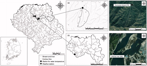
The YS is a first-order stream (i.e. within the T_w measuring station) that drains into an 0.234 km² area. The mean annual precipitation (mm ± standard deviation; SD) was 1354.4 ± 351.7 mm (minimum–maximum values: 696.5–2331.5 mm) according to the Palbong automatic weather station (AWS), 64% of which was concentrated in the summer season. Moreover, the mean annual temperature ± SD was 10.6 ± 0.5 °C (9.6–11.7 °C). Catchment elevations range from 335 to 658 m above the sea level. Additionally, 29% of the catchments were covered by coniferous trees (e.g. Pinus koraiensis, Larix leptolepis, and Pinus densiflora) and 71% by deciduous broad-leaved trees (e.g. Quercus spp., Fraxinus rhynchophylla, and Cornus controversa). Stream channels were 0.7 km in length, 0.6 m wide, and had a 0.24 m/m slope. The vegetation of the streamside consisted of riparian forest cover and an understory that changed to open and/or closed types with seasonal distribution.

The BR is a seventh-order river (i.e. within the T_w measuring station) that drains into a 4448.5 km² area. The mean annual precipitation ± SD from 1997 to 2018 at the Namsan AWS was 1358.5 ± 296.1 mm (717.5–2017.5 mm), 65% of which was concentrated in the summer season. Moreover, the mean annual temperature ± SD was 10.6 ± 0.5 °C (9.6–11.7 °C). The catchment elevations of this region range from 87 to 846 m above sea level. The river channels were 162.1 km in length, 1223.2 m wide, and had a 0.005 m/m slope. This patch on this riverside consisted of unforested land, the canopy of which was maintained as open type regardless of seasonal distribution.

Field monitoring and data analysis

Field measurements were carried out from April 20 to November 3 of 2017 and 2018. Measurements were not conducted in winter and early spring (i.e. from December to March), as stream and river watersheds freeze during this period. The T_w in the YS was monitored using a Yellow Springs Instruments (YSI) 6600 multisensor sonde at 1-hour intervals within 10 cm of the water surface. The T_w at the BR was monitored with a YSI 6600 EDS sonde; the measurements were taken within 50 cm of the water surface at 1-h intervals. The T_w data of the BR was obtained from Uiam station of the National Institute of Environmental Research (NIER) in South Korea. The daily T_A values for the YS and BR were obtained from each respective weather station in Yeonyeob and Kyegwan Mountains located close to the T_w monitoring points (Figure 1). Given the long distance between the weather stations for T_A measurements and the T_w point for the BR (> 10 km), a relatively nearby station was selected instead (Yeonyeob Mountain, 6.0 km).

The term “elasticity” employed herein originated in economics (e.g. price elasticity of demand) and was subsequently adopted by many disciplines as a measurement of responsiveness (Png 1999). This has become a popular tool among empiricists due to its independent units, which simplifies data analysis. Precipitation elasticity of streamflow is a well-known application of the concept of elasticity in hydrology, which is defined as a change in river flow in response to a proportional change in precipitation (i.e. Chiew 2006; Sankarasubramanian et al. 2001; Yang and Liu 2011). These parameters are calculated as follows: (1) $${\epsilon }_T=\mathit{median}\left(\frac{{(T_w)}_t-\overline{T_w}}{{(T_A)}_t-\overline{T_A}}\frac{\overline{T_A}}{\overline{T_W}}\right)$$(1) (2) $${\epsilon }_p=\mathit{median}\left(\frac{{(T_w)}_t-\overline{T_w}}{{(P_T)}_t-\overline{P_T}}\frac{\overline{P_T}}{\overline{T_W}}\right)$$(2)

Where $\overline{T_A},$ $\overline{P_T}$ and $\overline{T_W}$ are the daily T_A, P_T, and T_w mean values, respectively. (T_A)_t, (P_T)_t, and (T_w)_t are the T_A, P_T, and T_w at a given time t. The values of $(\frac{{(T_w)}_t-\overline{T_w}}{{(T_A)}_t-\overline{T_A}}\frac{\overline{T_A}}{\overline{T_W}})$ and $(\frac{{(T_w)}_t-\overline{T_w}}{{(P_T)}_t-\overline{P_T}}\frac{\overline{P_T}}{\overline{T_W}})$ were computed for each (T_A)_t, (T_w)_t and (P_T)_t, (T_w)_t pair using a daily time series data set (e.g. Khan et al. 2017). The median from the above-described formula provided the nonparametric estimate of ε_T and ε_P (e.g. Jiang et al. 2014; Khan et al. 2017). Our estimates for ε_T and ε_P were used for T_w responses of direction and strength from T_A and P_T during limited observation periods.

The ε_T and ε_P parameters have some advantages over other techniques, including that the entire ε_T and ε_P functions are characterized by their median value, which minimizes the impact of outliers such as extreme events (e.g. flood and drought), which primarily affect the regional biota (e.g. Jiang et al. 2014; Khan et al. 2017). These parameters are also dimensionless, which simplifies data analysis (Khan et al. 2017).

A two-sample Student’s t-test was used, depending on assumptions of normality and variance equality (e.g. Xiao et al. 2012), to compare the mean differences in ε_T and ε_P in the YS and BR. All statistical analyses were performed using the Statistical Package for Social Sciences (SPSS), version 24.

Results

Temporal variations in water temperature and climate conditions

Figure 2 illustrates the temporal changes in T_w and climate conditions (i.e. P_T, relative humidity, and T_A) in the YS and BR from April to November of 2017 and 2018. Changes in T_w varied seasonally, whereas the T_A seasonal changes in the two studied points remained similar (Figure 2(c,d)). The T_w responses in the two points were distributed with a relatively high variability range from spring to summer (May–July), which was linked to increases in T_A and P_T (Figure 2(a,c)). In contrast, these T_w responses exhibited a relatively narrow range from summer to fall (August–October), which was associated with decreases in T_A and P_T (Figure 2(a,c)). The differences between T_A and T_w were 4–6 °C higher in the YS than the BR during the summer and fall seasons (Figure 2(c,d)).

Figure 2. (a) One-day and cumulative precipitation, (b) relative humidity, (c) air temperature, and (d) water temperature in the Yeonyeop stream (YS) and Bukhan River (BR) from April to November 2017 and 2018. The dotted and shaded areas indicate values excluded due to data missing from the study sites.

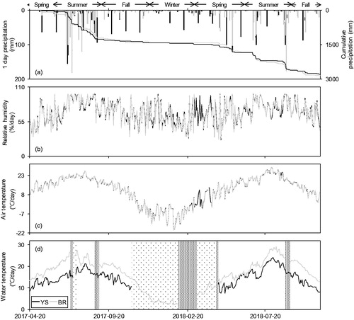
P_T during the observation period was 0.0–155.5 and 0.0–120.6 mm/day in the YS and BR, respectively (Table 1). The T_A during the observation period was 1.4–29.5 and 1.5–29.5 °C/day in the YS and BR, respectively, with 26.0–99.0 and 27.0–99.0%/day of relative humidity in the two study sites (Table 1). The T_w during the observation period was 7.5–24.1 °C/day in the YS and 12.2–29.3 °C/day in the BR (Table 1). Additionally, the mean T_A values and relative humidity were similar in both points, whereas the mean T_w value in the YS (4.7–5.2 °C/day) tended to be lower than in the BR. In contrast, greater mean P_T values were observed in the YS (0.0–34.9 mm/day) compared to the BR (Table 1).

Table 1. Summary of water temperature and other climate observations.

Site	n (days)	Precipitation (mm/day)	Relative humidity (%/day)	Air temperature (°C/day)	Water temperature (°C/day)
YS	391	7.3 ± 21.1 (0.0–155.5)	73.5 ± 16.0 (26.0–99.0)	17.1 ± 5.3 (1.4–29.5)	14.9 ± 3.7 (7.5–24.1)
BR	376	5.7 ± 17.4 (0.0–120.6)	72.9 ± 16.2 (27.0–99.0)	17.1 ± 5.4 (1.5–29.5)	19.7 ± 4.0 (12.2–29.3)

YS: Yeonyeop stream, BR: Bukhan River; ±: standard deviation, Bracket: minimum–maximum values.

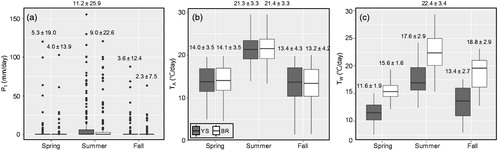
The seasonal mean values of P_T ± SD in the YS and BR were 5.3 ± 19.0 and 4.0 ± 13.9 mm/day in spring, 11.2 ± 25.9 and 9.0 ± 22.6 mm/day in summer, and 3.6 ± 12.4 and 2.3 ± 7.5 mm/day in the fall (Figure 3(a)). The seasonal mean values of T_A ± SD in the YS and BR were 14.0 ± 3.5 and 14.1 ± 3.5 °C/day in spring, 21.3 ± 3.3 and 21.4 ± 3.3 °C/day in summer, and 13.4 ± 4.3 and 13.2 ± 4.2 °C/day in the fall (Figure 3(b)). The seasonal mean values of T_w ± SD in the YS and BR were 11.6 ± 1.9 and 15.6 ± 1.6 °C/day in spring, 17.6 ± 2.9 and 22.4 ± 3.4 °C/day in summer, and 13.4 ± 2.7 and 18.8 ± 2.9 °C/day in the fall (Figure 3(c)). T_A and P_T exhibited seasonal differences between summer and both spring and fall with no spatial difference between the YS and BR. However, T_w exhibited variations in both seasonal and spatial distribution. Particularly, the T_w during the summer season was higher than that of the other two seasons. Moreover, the T_w in the YS was lower than that of the BR during the observation period (Figure 3(b,c)).

Figure 3. Seasonal changes in (a) precipitation (P_T), (b) air temperature (T_A), and (c) water temperature (T_w) at the Yeonyeop stream (YS) and Bukhan River (BR) from April to November 2017 and 2018.

Distribution of temperature and precipitation elasticities

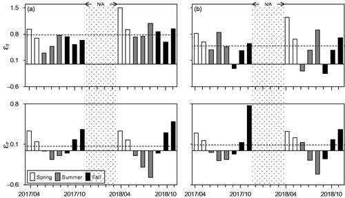
ε_T and ε_P in the YS and BR were calculated based on monthly data during the observation period (Figure 4). The ε_T ranged from 0.292 to 1.501 and from −0.253 to 1.243 in the YS and BR, respectively (Figure 4(a)). Moreover, the ε_P in the YS and BR ranged from −0.433 to 0.464 and −0.378 to 0.722 (Figure 4(b)). All ε_T values in the YS were positive values, whereas the ε_T values in the BR tended to be below the aforementioned value (–0.116 in September of 2017, −0.182 in June of 2018, and −0.253 in September of 2018). The ε_P values in the YS and BR were negative, ranging from −0.433 to −0.004, particularly from June to September (Figure 4(a,b)).

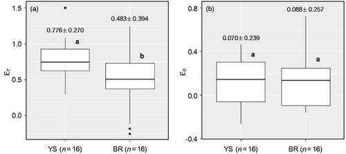
Figure 4. Elasticity distribution (ε_T: temperature elasticity, ε_P: precipitation elasticity) at the (a) Yeonyeop stream (YS) and (b) Bukhan River (BR) from April to November 2017 and 2018. The horizontal dashed lines indicate mean values of ε_T and ε_P. The dotted area indicates values that are not available (N/A) due to data missing from December to March of the study period.

The mean ε_T ± SD in the YS (0.776 ± 0.270) was greater than that in the BR (0.483 ± 0.394) (Figure 5(a)); however, the mean of ε_P ± SD in the YS (0.070 ± 0.239) was lower than the BR (0.088 ± 0.257) (Figure 5(b)). The differences in ε_T between the YS and BR were significant according to a two-sample Student’s t-test (t = 2.37, df = 30.00, p < 0.05); however, no differences were observed in the ε_P values of the two examined sites (Figure 5(a,b)).

Figure 5. (a) Temperature (ε_T) and (b) precipitation (ε_P) elasticities at the Yeonyeop stream (YS) and Bukhan River (BR) from April to November 2017 and 2018. A two-sample Student’s t-test is indicated in separate bold letters (a and b) above the box.

Comparison of seasonal changes in temperature and precipitation elasticities between two study sites

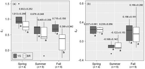
Figure 6 illustrates the mean values and ranges of ε_T and ε_P seasonal changes in the YS and BR. Mean ε_T and ε_P values in the YS and BR were higher in the spring than in both summer and fall. In particular, the ε_P mean value in the YS was lower than that in the BR, whereas the ε_T mean value in the YS was higher than that in the BR due to seasonal elasticity differences between the YS and BR (Figure 6). The difference in ε_T between the YS and BR during the fall season was significant according to a two-sample Student’s t-test (t = 2.67, df = 10.00, p < 0.05). Therefore, the seasonal differences between the ε_T values at the YS and BR were found to be significant (Figure 6(a)).

Figure 6. Seasonal changes in (a) temperature (ε_T) and (b) precipitation (ε_P) elasticities at the Yeonyeop stream (YS) and Bukhan River (BR) from April to November 2017 and 2018. Values above each box indicate mean ± standard deviation. A two-sample Student’s t-test is indicated in separate bold letters (a and b) above the box.

Based on the results in Figure 6, correlation analysis was performed between T_w and both ε_T and ε_P for each of the two study sites. T_w and both ε_T and ε_P were significantly correlated in the summer season for the two sites (correlation coefficient: −0.98–0.96, p < 0.05) (Table 2). Moreover, T_w and both ε_T and ε_P were negatively significantly correlated in the spring and fall seasons for the two sites (correlation coefficient: −0.997 – −0.85, p < 0.05), whereas T_w and ε_P were not significantly correlated in the spring season for the YS site (correlation coefficient: −0.92, p = 0.084) (Table 2).

Table 2. Correlation analysis of the seasonal differences between T_w (water temperature) and both temperature (ε_T) and precipitation (ε_P) elasticities at the Yeonyeop stream (YS) and Bukhan River (BR) from April to November 2017 and 2018.

Season	YS				BR
	εT		εP		εT		εP
Spring	–0.83	p = 0.174	–0.92	p = 0.084	–0.85	p = 0.151	–0.99	p = 0.009
Summer	0.92	p = 0.011	–0.93	p = 0.007	0.96	p = 0.002	–0.98	p = 0.001
Fall	–0.07	p = 0.898	–0.997	p < 0.01	–0.99	p < 0.01	–0.85	p = 0.032

YS: Yeonyeop stream, BR: Bukhan River; ε_T: temperature elasticity, ε_P: precipitation elasticity; Significant correlations are shown as bold type.

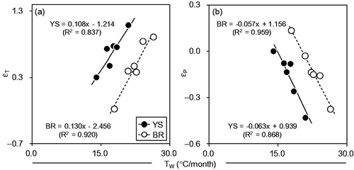
Moreover, the correlation analysis results indicated a relationship between T_w and both ε_T and ε_P for both study sites, albeit only during the summer season (Table 2 and Figure 7). In the two sites, the ε_T was increased with increasing T_w (Figure 7(a)), whereas the ε_P increased as T_w decreased (Figure 7(b)). Particularly, the T_w of the YS was more sensitive to T_A changes than that of the BR. Regression analysis between the two sites rendered significant results, with coefficients of determination (R²) ranging from 0.837 to 0.959 at a 95% significance level; however, the relationship between T_w and both ε_T and ε_P exhibited a different trend (Figure 7). As illustrated in Figure 7, the T_w and both the ε_T and ε_P in both the YS and BR were highly correlated both spatially and temporally, particularly summer season.

Figure 7. Relationship between water temperature (T_w) and both (a) temperature (ε_T) and (b) precipitation (ε_P) elasticities at the Yeonyeop stream (YS) and Bukhan River (BR) during the summer season from April to November 2017 and 2018.

Discussion

This study determined that T_w responses increased with T_A, and T_w variations were wider than those of T_A in both study sites during the monitoring period (Figure 2(c,d)). This indicated that the specific heat of the water was higher than that of the air, which is among the physical characteristics of air-water temperature relationships (Crisp and Howson 1982; Webb and Nobilis 1997). Interestingly, the variations in T_w versus T_A in the YS was wider than the BR (Figure 3(c)).

Previous studies have also characterized temporal variations in T_w as a function of T_A. For instance, Chikita (2018) reported that the daily mean T_A from July to August in a forest region (Putoisaroma Stream, Hokkaido, Japan) was 20 °C, whereas the daily mean T_w was 15 °C. Moore (2006) found that the T_w exhibited a year-round warming effect equivalent to  approximately 3–4 °C increase for each 10% increase in percent stream cover in the summer season in British Columbia, Canada. Nam et al. (2019) indicated that the daily mean T_w in nine forested headwater streams in Gangwon-do (South Korea) was approximately 6 °C lower than the daily mean T_A . Lane et al. (2007) demonstrated that T_w reached a high of > 30 °C in the summer and a low of < 12 °C in the winter in the Breton Sound estuary of the Mississippi River, USA. Webb (1996) also reported monthly mean T_A increases of 2 and 4 °C in the summer and winter seasons, which were projected to cause monthly mean T_w increases from 1.1 to 2.2 °C in the Lambourn River of southern England, UK. Consequently, these relationships between T_A and T_w suggest that increases in T_w following increases in T_A are predominantly moderated by the influence of seasonal environmental variations on water surface temperature in forested headwater streams and lowland rivers (e.g. Mackey and Berrie 1991; Webb 1996).

In both study sites, seasonal variations in P_T, T_A, and T_w exhibited higher temperatures in the summer season than in the spring and fall (Figure 3). This demonstrated that the T_w reached a maximum as a function of T_A due to seasonal impacts from June to August; however, the T_w in the forested headwater stream, which became the steeper slope during repetitive heavy rain and drought processes, originated from potential direct and/or indirect runoff (Park and Lee 2000; Moore 2006). Moreover, the latent heat of vaporization of the water surface was higher in the summer season than the winter, in addition to the seasonal effects of input streams and rivers, groundwater, or melting snow water (Stefan and Preud’homme 1993; Milner et al. 2009; Łaszewski 2018).

Particularly, the difference between T_A and T_w was greater in the YS than the BR both in the summer and fall seasons (Figure 2(c,d)). This was because topographic and geological conditions in the YS had steep side slopes and the contributions from the riparian zone remained shaded, thereby exerting cooling and humidifying effects (e.g. Cho et al. 2007; Isaak et al. 2012). In particular, deciduous broad-leaved trees (79% of the catchment) in the YS provide significant amounts of shade because of their heights and extensive canopies over the riparian zone (Gregory et al. 1991; Beschta 1997; Dugdale et al. 2018). In addition, shading can also be generated by topography and/or the stream channel (Larson and Larson 1996; Garner 2017). Instream flows to increase stream shading could also offset significant amounts of future warming where headwater forested stream riparian zone degradation is severe (Meier et al. 2003; Moore et al. 2005). For instance, Nakamura and Dokai (1989) found that differences in the daily T_w under the same solar radiation conditions during the defoliation period were greater than in the foliation period. Sinokrot and Stefan (1993) also reported that the percentage exposure of the stream surface to the sun was greater in early spring and fall when leaves were absent. Additionally, the riparian zone may be narrow to nonexistent, because the YS site examined herein had topographic constraints imposed by steep side slopes on the headwater stream (Richardson et al. 2005). Mountain regions can contribute to the development of drainage winds that flow down valleys and gullies (Oke 1987), advecting cool air into lower reaches such as lowland rivers located in urban areas. Thus, given that the YS was studied for both its narrow riparian zone and near steep side slopes, the temporal variation in T_w for YS was different compared to the BR (Figure 2). Different amounts of solar radiation or shading between the YS and BR also could be highly correlated with the relatively high altitude (373 m) and open and/or close condition of the riparian forest cover with understory vegetation in the streamside of forested headwater streams (Pluhowski 1972; Becker et al. 2004; Webb et al. 2008; Steel et al. 2016). Previous studies have shown that a combination of topography factors can substantially alter the behaviors of flow paths in streams and rivers within a given basin (e.g. Huang et al. 2008; Vanderhoof and Lane 2019).

Seasonal T_w responses were apparent in both the ε_T and ε_P values of the YS and BR, particularly during the summer season (Table 2). Here, ε_T increased with increases in T_w, whereas ε_P increased with decreases in T_w (Figure 7). Similarly, Dooge (1992) reported that elasticity could become stronger with declining precipitation, in addition to indicating water limitations. Jiang et al. (2014) reported that the ε_P exhibited higher spatial variability than ε_T, and seasonal changes were also more evident for ε_P than ε_T. With temporal and spatial variations, Shon et al. (2010) indicated that the ε_T increased with water velocity and water surface area from upper to lower reaches in the Nakdong River watershed. The ε_T value in the BR site studied herein was low due to decreased water velocity and a long channel length (151 km) with a relatively low slope (0.005 m/m). However, the T_w of the YS, which was within a forested headwater, was more sensitive to T_A changes due to its hydrologic and geological conditions (i.e. channel length (0.7 km) and steep slope (0.24 m/m) in the riparian zone) (e.g. Moore et al. 2005).

Additionally, the riparian zone transitions from the hydrophilous vegetation characteristic of the wetted edge to the understory vegetation of the upslope forest, enhancing the range of physical conditions (Richardson et al. 2005). For instance, Creed et al. (2014) demonstrated that the ε_T and ε_P values would respond to forest types and ages such that they would have the capacity to adapt to changing climatic conditions. Given the nature of these spatial characteristics, our study employed existing empirical datasets from the YS and BR to draw inferences about the influence of temporal and spatial variations on T_w changes, even if we only had limited case study from the Bukhan River basin, South Korea. Furthermore, studying the response of T_w to precipitation and T_A from an elasticity standpoint may establish a methodological and theoretical basis for the development of sustainable water management strategies in the riparian zone by accounting for relevant influencing factors such as the magnitude of the canopy opening in the forest and the adjacent hillside slopes (e.g. Wimberly and Spies 2001; Richardson et al. 2005; Razak et al. 2009).

Summary and conclusions

This study investigated the effect of air temperature and precipitation on the water temperature of Yeonyeop stream (YS), a forested headwater stream, and Bukhan River (BR), an urban river within the same basin from 2017 to 2018. Our main findings were the following: (1) the differences between air and water temperatures were 4–6 °C higher in the YS than the BR during the summer and fall seasons; (2) air temperature and precipitation presented seasonal differences with no apparent spatial variation; however, water temperature varied both seasonally and spatially; (3) the mean value of temperature elasticity ± standard deviation in the YS (0.776 ± 0.270) was greater than that of the BR (0.483 ± 0.394), whereas the mean value of precipitation elasticity in the YS (0.070 ± 0.239) was lower than that of the BR (0.088 ± 0.257); (4) a statistically significant difference between the temperature elasticity of the YS and BR was identified at a 95% confidence level (p < 0.05) even if no differences in precipitation elasticity were identified between the two sites; (5) based on water temperature and both temperature and precipitation elasticities, temperature elasticity increased with increases in water temperature during summer, whereas precipitation elasticity increased with decreases in water temperature; and (6) the water temperature of the YS was more sensitive to air temperature compared to the BR from an elasticity perspective.

Therefore, the seasonal variations in water temperature observed herein were attributed to elasticity responses due to the effect of irregular and intermittent flow conditions with extremely low and high flows (e.g. Bryant et al. 2007; Collins et al. 2007) for a forested headwater stream. Although this study was limited both in terms of spatial and temporal scales, the unique aspects of our study design allowed for the creation of inferences regarding the resilience of forested headwater streams and urban rivers to ecological and hydrological characteristics that may influence their response. Furthermore, our findings will likely be useful for sustainable water resources management, where impacts from anthropogenic factors need to be minimized. Given that the sensitivity of water temperature to air temperature depended largely on spatial characteristics that had temporal variations, sustainable water management plans should incorporate long-term monitoring sites within forested headwater streams as the main source of water in the context of river connectivity.

Acknowledgements

We would like to thank the National Institute of Environmental Research for assistance in the provision of observation data. We also appreciate helpful comments from the anonymous reviewers.

Disclosure statement

No potential conflict of interest was reported by the author(s).

Additional information

Funding

This research was supported by Korea Ministry of Environment as part of “The SS (Surface Soil conservation and management) projects; 2019002830002” and the National Research Foundation (NRF) grant funded by the Korea government (MSIT) (No. NRF-2017R1C1B5076781).

References

- Agudelo‐Vera C, Avvedimento S, Boxall J, Creaco E, de Kater H, Di Nardo A, Djukic A, Douterelo I, Fish K, Iglesias Rey PL, et al. 2020. Drinking water temperature around the globe: understanding, policies, challenges and opportunities. Water. 12(4):1049.
- Arismendi I, Johnson SL, Dunham JB, Haggerty R. 2013. Descriptors of natural thermal regimes in streams and their responsiveness to change in the Pacific Northwest of North America. Freshw Biol. 58(5):880–894.
- Arnell N. 1996. Global warming, river flows and water resources. Chichester, West Sussex, UK: Wiley.
- Becker M, Georgian T, Ambrose H, Siniscalchi K, Fredrick K. 2004. Estimating flow and flu of ground water discharge using water. J Hydrol. 296(1-4):221–233.
- Beschta RL. 1997. Riparian shade and stream temperature: an alternative perspective. Rangelands. 19:25–28.
- Beschta RL, Bilby RE, Brown GW, Holtby LB, Hofstra TD. 1987. Stream temperature and aquatic habitat: fisheries and forestry interactions. In: Salo EO, Cundy TW, editors. Streamside management: forestry and fishery interactions. Seattle, WA: University of Washington, Institute of Forest Resources, Contribution No. 57; p. 191–232.
- Bettinger P, Siry J, Merry K. 2013. Forest management planning technology issues posed by climate change. Forest Sci Technol. 9(1):9–19.
- Brown LE, Hannah DM, Milner AM. 2006. Hydroclimatological influences on water column and streambed thermal dynamics in an alpine river system. J Hydrol. 325(1–4):1–20.
- Bryant M, Gomi T, Piccolo J. 2007. Structures linking physical and biological processes in headwater streams of the Maybeso watershed, Southeast Alaska. For Sci. 53:371–383.
- Caissie D. 2006. The thermal regime of rivers: a review. Freshwater Biol. 51(8):1389–1406.
- Cayan DR, Riddle LG, Aguado E. 1993. The influence of precipitation and temperature on seasonal streamflow in California. Water Resour Res. 29(4):1127–1140.
- Chiew FHS. 2006. Estimation of rainfall elasticity of streamflow in Australia. Hydrol Sci J. 51(4):613–625.
- Chikita KA. 2018. Environmental factors controlling stream water temperature in a forest catchment. AIMS Geosci. 4:192–214.
- Cho HY, Lee KH, Cho KJ, Kim JS. 2007. Correlation and hysteresis analysis between air and water temperatures in the Coastal Zone – Masan Bay. J Korean Soc Mar Environ. 19:213–221. (in Korean with English abstract).
- Chong SK, Kim HH, Won HK. 2006. Case study for sustainable management of Jeju experimental forest. Forest Sci Technol. 2(2):73–79.
- Collins BM, Sobczak WV, Colburn EA. 2007. Subsurface flowpaths in a forested headwater stream harbor a diverse macroinvertebrate community. Wetlands. 27(2):319–325.
- Creed IF, Spargo AT, Jones JA, Buttle JM, Adams MB, Beall FD, Booth EG, Campbell JL, Clow D, Elder K, et al. 2014. Changing forest water yields in response to climate warming: results from long-term experimental watershed sites across North America. Glob Chang Biol. 20(10):3191–3208.
- Crisp DT, Howson G. 1982. Effect of air temperature upon mean water temperature in streams in the north Pennies and English Lake District. Freshw Biol. 12(4):359–367.
- Dallas H, Day J, Musibono D, Day E. 1998. Water quality for aquatic ecosystems: tools for evaluating regional guidelines, Report No. 626/1/98. Pretoria, South Africa: Water Research Commission.
- Dizon JT, Calderon MM, Camacho LD, Carandang MG, Rebugio LL, Tolentino NM. 2006. Institutionalization of a water user fee for watershed management. Forest Sci Technol. 2(1):51–56.
- Dugdale SJ, Malcolm IA, Kantola K, Hannah DM. 2018. Stream temperature under contrasting riparian forest cover: understanding thermal dynamics and heat exchange processes. Sci Total Environ. 610-611:1375–1389.
- Dooge JCI. 1992. Sensitivity of runoff to climate change: a Hortonian approach. Bull Amer Meteor Soc. 73(12):2013–2024.
- Eaton JG, Scheller RM. 1996. Effects of climate warming on fish thermal habitat in streams of the United States. Limnol Oceanogr. 41(5):1109–1115.
- Ficklin DL, Barnhart BL, Knouft JH, Stewart IT, Maurer EP, Letsinger SL, Whittaker GW. 2014. Climate change and stream temperature projections in the Columbia River basin: habitat implications of spatial variation in hydrologic drivers. Hydrol Earth Syst Sci. 18(12):4897–4912.
- Fullerton AH, Torgersen CE, Lawler JJ, Faux RN, Steel EA, Beechie TJ, Ebersole JL, Leibowitz SG. 2015. Rethinking the longitudinal stream temperature paradigm: region-wide comparison of thermal infrared imagery reveals unexpected complexity of river temperatures. Hydrol Process. 29(22):4719–4737.
- Garner G, Malcolm IA, Sadler JP, Hannah DM. 2017. The role of riparian vegetation density, channel orientation and water velocity in determining river temperature dynamics. J Hydrol. 553:471–485.
- Gregory SV, Swanson EJ, McKee WA, Cummins KW. 1991. An ecosystem perspective of riparian zones: focus on links between land and water. Bioscience. 41(8):540–551.
- Hlúbiková D, Novais MH, Dohet A, Hoffmann L, Ector L. 2014. Effect of riparian vegetation on diatom assemblages in headwater streams under different land uses. Sci Total Environ. 475:234–247.
- Huang M, Liang X, Leung LR. 2008. A generalized subsurface flow parameterization considering subgrid spatial variability of recharge and topography. J. Hydrometeorol. 9(6):1151–1171.
- Inoue M, Nakano S, Nakamura F. 1997. Juvenilemasu salmon (Oncorhynchus masou) abundance and stream habitat relationships in northern Japan. Can J Fish Aquat Sci. 54(6):1331–1341.
- Isaak DJ, Wollrab S, Horan D, Chandler G. 2012. Climate change effects on stream and river temperatures across the northwest U.S. from 1980–2009 and implications for salmonid fishes. Clim Change. 113(2):499–524.
- Jiang J, Sharma A, Sivakumar B, Wang P. 2014. A global assessment of climate-water quality relationships in large rivers: an elasticity perspective. Sci Total Environ. 468–469:877–891.
- Johnson SL. 2004. Factors influencing stream temperatures in small streams: substrate effects and a shading experiment. Can J Fish Aquat Sci. 61(6):913–923.
- Jun JH, Kim KH, Yoo JY, Choi HT, Jeong YH. 2007. Variation of suspended solid concentration, electrical conductivity and pH of stream water in regrowth and rehabilitation forested catchments, South Korea. J Korean For Soc. 96:21–28. (in Korean with English abstract).
- Khan A, Jiang J, Sharma A, Wang P, Khan J. 2017. How do terrestrial determinants impact the response of water quality to climate drivers? – an elasticity perspective on the water–land–climate nexus. Sustainability. 9(11):2118–2128.
- Kim IJ, Han DH. 2008. A small stream management plan to protect the aquatic ecosystem. Sejong, Republic of Korea: Korea Environment Institute. (in Korean).
- Korea Forest Service (KFS). 2019. Statistical yearbook of forestry 2019. Daejeon, Korea: Korea Forest Service. (in Korean).
- Lane R, Day JW, Marx B, Reyes E, Hyfield E, Day JN. 2007. The effects of riverine discharge on temperature, suspended sediments, and chlorophyll a in a Misssissippi delta estuary measured using a flow-through system. Estuar Coast Shelf Sci. 74(1–2):145–154.
- Larson LL, Larson SL. 1996. Riparian shade and stream temperature: a perspective. Rangelands. 18:115–149.
- Łaszewski M. 2018. Human impact on spatial water temperature variability in lowland rivers: a case study from Central Poland. Pol J Environ Stud. 27(1):191–200.
- Lee S, Klein A, Over T. 2004. Effects of the El Niño–southern oscillation on temperature, precipitation, snow water equivalent and resulting streamflow in the Upper Rio Grande river basin. Hydrol Process. 18(6):1053–1071.
- Macan TT. 1974. Freshwater ecology. 2nd ed. London: Longman Group.
- MacDonald LH, Coe D. 2007. Influence of headwater streams on downstream reaches in forested areas. For Sci. 53:148–168.
- Mackey AP, Berrie AD. 1991. The prediction of water temperatures in chalk streams from air temperatures. Hydrobiologia. 210(3):183–189.
- Malcolm IA, Soulsby C, Youngson AF. 2002. Thermal regime in the hyporheic zone of two contrasting salmonid spawning streams: Ecological and hydrological implications. Fisheries Manag Ecol. 9(1):1–10.
- Meier W, Bonjour C, Wüest A, Reichert P. 2003. Modeling the effect of water diversion on the temperature of mountain streams. J Environ Eng. 129(8):755–764.
- Milner AM, Brown LE, Hannah DM. 2009. Hydroecological response of river systems to shrinking glaciers. Hydrol Process. 23(1):62–77.
- Moore RD. 2006. Stream temperature patterns in British Columbia, Canada, based on routine spot measurements. Can Water Resour. J. 31(1):41–56.
- Moore RD, Spittlehouse DL, Story A. 2005. Riparian microclimate and stream temperature response to forest harvesting: a review. J Am Water Resources Assoc. 41(4):813–834.
- Nakamura F, Dokai T. 1989. Estimation of the effect of riparian forest on stream temperature based on heat budget. J Jap Forestry Soc. 71:387–394. (in Japanese with English abstract).
- Nam S, Choi HT, Lim H. 2019. Seasonal variations of stream water temperature and its affecting factors on mountain areas. J Korean Soc Water Environ. 35:308–315. (in Korean with English abstract).
- Oke TR. 1987. Boundary layer climates. 2nd ed. London, UK: Halsted Press; p. 1–435.
- Padilla A, Rasouli K, Déry SJ. 2015. Impacts of variability and trends in runoff and water temperature on salmon migration in the Fraser River Basin. Canada Hydrol Sci J. 60(3):523–533.
- Park JC, Lee HH. 2000. Variations of stream water quality caused by discharge change. J Korean For Soc. 89:342–355. (in Korean with English abstract).
- Pluhowski EJ. 1972. Hydrologic interpretations based on infrared imagery of Long Island, New York, U.S., Survey Water-Supply Paper 2009-B; p. 1–20.
- Png I. 1999. Managerial economics. Oxford: Blackwell.
- Poole GC, Berman CH. 2001. An ecological perspective on in-stream temperature: natural heat dynamics and mechanisms of human-caused thermal degradation. Environ Manage. 27(6):787–802.
- Rajwa-Kuligiewicz A, Bialik RJ, Rowiński PM. 2015. Dissolved oxygen and water temperature dynamics in lowland rivers over various timescales. J Hydrol Hydromech. 63(4):353–363.
- Razak SA, Son Y, Lee WK, Cho Y, Noh NJ. 2009. Afforestation and reforestation with the clean development mechanism: potentials, problems, and future directions. Forest Sci Technol. 5(2):45–56.
- Richardson JS, Naiman RJ, Swanson FJ, Hibbs DE. 2005. Riparian communities associated with Pacific Northwest Headwater Streams: assemblages, processes, and uniqueness. J Am Water Resources Assoc. 41(4):935–947.
- Sankarasubramanian A, Vogel RM, Limbrunner JF. 2001. Climate elasticity of streamflow in the United States. Water Resour Res. 37(6):1771–1781.
- Sato T, Watanabe K, Arizono M, Mori S, Nagoshi M, Harada Y. 2008. Intergeneric hybridization between sympatric Kirikuchi char and red-spotted masu salmon in a small Japanese mountain stream. N Am J Fish Manag. 28(2):547–556.
- Shin JH, Chun JH. 2011. Forest monitoring in times of climate change from the Asian view. Forest Sci Technol. 7(2):47–52.
- Shon TS, Lee YG, Baek MK, Shin HS. 2010. Analysis for air temperature trend and elasticity of air-water temperature according to climate changes in Nakdong River Basin. J Korean Soc Water Qual. 26:822–833. (in Korean with English abstract).
- Sinokrot BA, Stefan HG. 1993. Stream temperature dynamics: measurements and modeling. Water Resour Res. 29(7):2299–2312.
- Stefan HG, Preud'homme EB. 1993. Stream temperature estimation from air temperature. J Am Water Resour Assoc. 29(1):27–45.
- Stefan HG, Sinokrot BA. 1993. Projected global climate change impact on water temperatures in five north central US stream. Climate Change. 24(4):353–381.
- Steel EA, Sowder C, Peterson EE. 2016. Spatial and temporal variation of water temperature regimes on the Snoqualmie River network. J Am Water Resour Assoc. 52:1–19.
- Suzuki K. 2018. Importance of hydro-meteorological observation in the mountainous area. Jpn J Mt Res. 1:1–11. (in Japanese with English abstract).
- Vanderhoof MK, Lane CR. 2019. The potential role of very high-resolution imagery to characterize lake, wetland and stream systems across the Prairie Pothole Region, United States. Int J Remote Sens. 40(15):5768–5798.
- Vannote RL, Sweeney BW. 1980. Geographic analysis of thermal equilibria: a conceptual model for evaluating the effect of natural and modified thermal regimes on aquatic insect communities. Am Nat. 115(5):667–695.
- Ward JV. 1985. Thermal characteristics of running waters. Hydrobiologia. 125(1):31–46.
- Webb BW. 1996. Trends in stream and river temperature. Hydrol Process. 10(2):205–226.
- Webb BW, Clack PD, Walling DE. 2003. Water–air temperature relationships in a Devon river system and the role of flow. Hydrol Process. 17(15):3069–3084.
- Webb BW, Hannah DW, Moore RD, Brown LE, Nobilis F. 2008. Recent advances in stream and river temperature research. Hydrol Process. 22(7):902–918.
- Webb BW, Nobilis F. 1997. Long term perspective on the nature of the air-water temperature relationship: a case study. Hydrol Process. 11(2):137–147.
- Williams MW, Losleben M, Caine N, Greenland D. 1996. Changes in climate and hydrochemical responses in a high elevation catchment in the Rocky Mountains, USA. Limnol Oceanogr. 41(5):939–946.
- Wimberly MC, Spies TA. 2001. Influences of environment and disturbance on forest patterns in Coastal Oregon Watersheds. Ecology. 82(5):1443–1459.
- Xiao F, Halbach TR, Simcik MF, Gulliver JS. 2012. Input characterization of perfluoroalkyl substances in wastewater treatment plants: source discrimination by exploratory data analysis. Water Res. 46(9):3101–3109.
- Yang ZF, Liu Q. 2011. Response of streamflow to climate changes in the yellow river basin. China J Hydrometeorol. 12(5):1113–1126.