Thirty-two years of mangrove forest land cover change in Parita Bay, Panama

Abstract

Mangrove forests have experienced a rapid decline. However, the rate of loss has decreased in recent years due to enhanced conservation and nature regeneration. The dynamics of mangrove forests in Panama have not been monitored since the year 2000, despite a significant loss during the 1980s. The objectives of our study were to quantify changes in mangrove cover and identify the dominant drivers of change in Parita Bay, Panama. Temporal changes in mangrove cover and the Normalized Difference Vegetation Index (NDVI) were determined using the supervised classification method on Landsat satellite images from 1987 to 2019. We identified a 4.7% increase in the mangrove area of Parita Bay during the 32 years; the mangrove forests were also considered healthy as reflected by high NDVI values. However, the conversion of mangroves to other land cover types resulted in a 1.26% decline in mangrove cover from 1987 to 1998. Moreover, the area of aquaculture and saltpans almost doubled during this period. During the following two decades, the conversion of other land cover classes (water, other vegetation, and bare soil) increased the mangrove area by 6%, and the annual rate of increase was greater during the second decade (0.43% year⁻¹). From 2009 to 2019, mangroves declined at an annual rate of 0.11% in protected areas and increased at an annual rate of 0.50% in unprotected areas. Despite the regeneration potential of mangrove forests, our study highlights the need to continually manage and protect mangrove forests in order to facilitate their expansion in Parita Bay.

Keywords:

• Mangroves
• remote sensing
• land use-cover change (LUCC)
• Normalized Difference Vegetation Index (NDVI)
• aquaculture
• Panama

1. Introduction

Mangrove forests comprise 73 species and cover a total area of ∼152,000 km² globally, spanning 123 countries (Spalding 2010). Mangroves comprise halophytic trees, shrubs, and plants located in the critical interface between terrestrial, estuarine, and near-shore marine ecosystems in the tropics and subtropics (between latitudes 35°N and 38°S) (Polidoro et al. 2010; Kauffman and Donato 2012; Alatorre et al. 2016; Thomas et al. 2017; Kamruzzaman et al. 2019). They provide numerous important ecosystem services, including nurseries for marine species, sediment stabilization, water purification, woody and non-woody forest products, biological conservation, coastal protection, and the highest rates of carbon sequestration (Friess 2016; Rioja-Nieto et al. 2017; Godoy et al. 2018; Kamruzzaman et al. 2019; Afonso et al. 2021). Mangroves are one of the most effective carbon sink forests; they store an average of 937 t C ha⁻¹ and promote sediment deposition (∼5 mm year⁻¹) and carbon burial (174 g C m⁻²year⁻¹) (Alongi 2012). In addition, mangrove forests and their soils sequester approximately 22.8 million metric tons of carbon each year worldwide (Giri et al. 2011). Despite their many ecosystem benefits, mangroves are facing numerous threats, such as upstream pollution, timber extraction, land use change (mostly to aquaculture shrimp ponds), extreme weather events, sea-level rise, and precipitation and temperature variability (Gilman et al. 2008; McGowan et al. 2010; Donato et al. 2011; Valderrama-Landeros et al. 2017; Brown et al. 2018; Hsu and Lee 2018).

The stability of mangrove ecosystems is therefore under threat, as more than 1646 km² of world’s mangrove area has been lost from 2000 to 2012 (Hamilton and Casey 2016). There is a rising concern regarding mangrove vulnerability, with some studies projecting the total disappearance of mangrove forests within 100 years (Gilman et al. 2006; Duke et al. 2007; Alongi 2008; Gilman et al. 2008). However, the global rate of mangrove loss has declined overtime, and the carbon losses have reduced due to conservation policies, restoration projects, and the natural regeneration of mangrove species (Giri et al. 2011; Hamilton and Casey 2016; Thomas et al. 2017). Some studies have also reported increasing trends of mangrove forests in different parts of the world (Nursamsi and Komala 2017; Hsu and Lee 2018; Wang et al. 2018). It is, therefore, necessary to adequately monitor the dynamics of mangrove ecosystems to further understand their behavior, resilience, and future risks so that effective coastal adaptation and conservation policies can be implemented (e.g. protected areas).

Remote sensing tools are predominantly applied to monitor mangrove forests across the globe by assessing changes in mangrove area (Ghosh et al. 2017; Nursamsi and Komala 2017; Gaw et al. 2018; Godoy et al. 2018; Servino et al. 2018; Yoo et al. 2019); however, it is also necessary to assess the quality of mangrove forests to better understand their health status. The Normalized Difference Vegetation Index (NDVI) is the most commonly applied tool for assessing the quality of vegetation coverage—including that of mangrove forests (Seto and Fragkias 2007; Kuenzer et al. 2011; Wulder and Franklin 2012; Yengoh et al. 2015; Castillo et al. 2017; Flores-Cárdenas et al. 2018). For example, NDVI trends have been used to assess forest dieback in response to hailstorms and to determine vegetation degradation with increasing distance from shrimp farms (e.g. Alatorre et al. 2016; Servino et al. 2018). In this study, we used an NDVI time series together with Land Use Cover Change (LUCC) to monitor Panama’s mangrove coverage over the past three decades.

Panama’s mangrove forests are one of the most threatened globally, as they are located in both the Atlantic and Pacific Coasts of Central America (Polidoro et al. 2010). Ninety-seven percent of Panama’s mangrove forests is distributed on its Pacific side, and the remaining 3% is distributed on its Caribbean coast (CREHO-Ramsar 2009). Panama has the 16^th largest area of mangrove forests in the world, covering a total of 174,790 ha in 2012 (FAO 2015; Hamilton and Casey 2016). However, the country has experienced a significant loss in mangrove area from 360,000 ha in 1969 to approximately 170,000 ha in 2007 (ANAM and ARAP 2013). Despite the importance of mangrove conservation in the country, there is currently an absence of remote sensing monitoring data on mangrove coverage since the year 2000 (McGowan et al. 2010). The main objectives of this study are therefore to (1) quantify the extent and rate of change in mangrove coverage (gain and loss) over the last 32 years (1987–2019) in Parita Bay, Panama, (2) determine changes in mangrove quality by analyzing NDVI trends, and (3) identify the potential drivers of mangrove change and determine the differences in mangrove dynamics between protected and unprotected areas. Our study aims to provide information for policy makers to improve upon current mangrove conservation measures in Panama.

2. Material and methods

2.1. Study area

The study site is Parita Bay (between latitude 8°18′40″N and longitude 80°13′37″W to latitude 7°57′18″N and longitude 80°21′49″W) located on the central Pacific coast of Panama (Figure 1). The study area spans the provinces of Coclé, Herrera, and Los Santos and is part of the country’s “Dry Arc” (the driest zone of the country) region. The study area comprises five watersheds with a total area of approximately 613 km². The zone is characterized by dry tropical and dry premontane forests and has an annual precipitation of <1000 mm (ANAM and UCCD 2009). The most common mangrove species in the region include Laguncularia racemosa, Rhizophora mangle, Avicennia germinans, Conocarpus erectus, and Pelliciera rhizophorae (ANAM and ARAP 2013).

Figure 1. Location of the study area showing (a) the study site in Parita Bay, Panama; (b) the locations of the meteorological stations in the study site; and (c) the location of the protected areas: Cenegon de Mangle Wildlife Refuge and Sarigua National Park. Source: ESRI satellite. Quick Map Services.

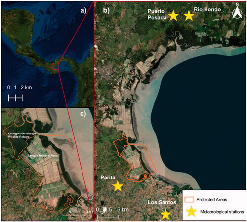
There are two protected areas within the study zone (Figure 2):

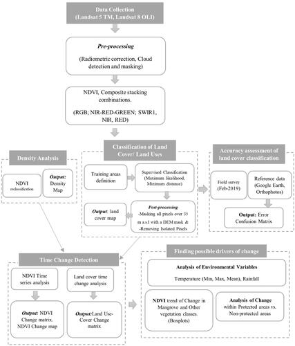
Figure 2. Flowchart of the study.

1. The Sarigua National Park. The park was established in 1984 with a total area of 47 km² or 80 km² when including the sea territory in Parita Bay. More than 50% of the protected area is used as shrimp-breeding ponds. The site is located in an archaeological area for the study of the cultural evolution of the Isthmus of Pre-Hispanic Panama (CREHO-Ramsar 2009).

2. Cenegon de Mangle Wildlife Refuge. The refuge was established in 1980 with an approximate area of 9 km². The region borders the Sarigua National Park and harbors the largest white ibis (Eudocimus albus) and large egret (Ardea alba) colonies in Panama as well as one of the largest heron colonies (CREHO-Ramsar 2009).

2.2. Data selection and image preprocessing

Five Landsat images with 30 m spatial resolution were downloaded from the United States Geological Survey’s (USGS) Earth Explorer website (https://earthexplorer.usgs.gov/) (Table 1). All five images were taken during the country’s dry season from December to April (UNESCO 2008). We used the surface reflectance products from the USGS Landsat Ecosystem Disturbance Adaptive Processing System (LEDAPS) (USGS 2018) and the Landsat Surface Reflectance Code (LaSRC) (USGS 2017) for atmospheric and radiometric corrections; these datasets are currently the most high-level and reliable products for atmospheric correction (Young et al. 2017).

Table 1. Data products used in this study.

Satellite	Sensor	Product ID	Date	Path/row
Landsat 5	TM	LT05_L1TP_012054_19870119_20170215_01_T1	1987-01-19	12/54
Landsat 5	TM	LT05_L1TP_012054_19980322_20161226_01_T1	1998-03-22	12/54
Landsat 5	TM	LT05_L1TP_012054_20091201_20161017_01_T1	2009-12-01	12/54
Landsat 5	TM	LT05_L1TP_012054_20100118_20161017_01_T1	2010-01-18	12/54
Landsat 8	OLI	LC08_L1TP_012054_20190127_20190206_01_T1	2019-01-27	12/54

Each band image was clipped to extract the cloud-free study region for the classification analysis. However, due to the absence of cloud-free conditions in 2009, we created a composite of the December 2009 and January 2010 images by combining their cloud-free areas. Each clipped band image was used to construct a composite for the classification. The False Color combination of Near-Infrared (NIR), RED, and GREEN as RGB were used to map the mangrove area on the 1987, 1998, and 2019 images (Jayanthi et al. 2018; Islam et al. 2019). Compared with other band combinations, the Short Wave Infrared (SWIR), NIR, and RED combination showed the best results for mapping mangroves on the 2009–2010 composite image (Rahman et al. 2017; Gaw et al. 2018).

2.3. Image classification and change detection

Images were classified using the supervised maximum likelihood algorithm for 1987, 1998, and 2019 based on the performance of the algorithms; only the 2009–2010 composite image was classified using the supervised classification via the minimum distance algorithm (Figure 2). We defined a new set of training areas for each satellite imagery. The land cover-land use map from the Ministry of Environment of Panama for the year 2012 was used as a reference for the definition of training areas and classification.

Five land cover-land use classes were defined: 1) Mangrove, 2) Water (rivers, ponds, sea), 3) Aquaculture Ponds and Salt Pans (AS), 4) Other Vegetation (grassland, shrubs, crops, upland forest, flood vegetation), and 5) Bare Soil & Built-Up (BB). We performed a visual classification for the AS category (Alatorre et al. 2016; Jayanthi et al. 2018; Thomas et al. 2017). Following land cover classification, we performed image post processing to remove isolated pixels. Panama’s mangroves grow up to 30 m (ANAM and ARAP 2013) and occur in intertidal areas at < 5 m a.s.l. (Gaw et al. 2018). All mangrove pixels located at high elevations (>35 m a.s.l.) were therefore masked using the digital elevation model of the Shuttle Radar Topography Mission (SRTM; 1-arc resolution). All tasks related to classification, raster edition, dilation, LUCC, and NDVI reclassification were developed in QGIS 3.4 and 2.18 (http://qgis.osgeo.org/) using the semi-automatic classification (Congedo 2016) plugin and Modules of Land Use Change Evaluation (MOLUSCE) plugin (Rahman et al. 2017).

We also performed additional LUCC detection for protected and unprotected areas. All images were masked with the protected areas “Cenegon de Mangle Wildlife Refuge” and “Sarigua National Park” shapefiles provided by the Ministry of Environment of Panama.

2.4. Field ground truth and accuracy assessment

A field survey was performed during February 8–12, 2019 to assess the accuracy of the 2019 image. The reference data must be independent from the data being tested to ensure assessment objectivity (Clevers 2009). Field data obtained from the ground observations were therefore only used for the accuracy assessment and not in the setting of training areas for the supervised classification. We used Garmin GPSMAP 64S to perform stratified random sampling near to roads or access ways, as some areas had restricted or dangerous access due to dense mangrove zones (Clevers 2009). We obtained a total of 250 validation points (125 field validation points and 125 Google Earth validation points) for the 2019 image (Tilahun and Teferie 2015). We performed a similar process for the 2009–2010 image by validating 250 random sample points using Google Earth images and orthophotography from 2009 provided by the Ministry of Environment of Panama. A pixel-based error matrix and Kappa coefficient were calculated. Images from 1987 and 1998 were not validated due to the lack of data.

2.5. NDVI analysis

In addition to the land use-cover classification, we also performed an NDVI reclassification to quantify the mangrove quality change over time. NDVI was calculated for each satellite image using the following equation Rouse et al. (1974): (1) $$\text{NDVI}=\frac{\mathit{NIR}\hspace{0.17em}-\hspace{0.17em}\mathit{RED}}{\mathit{NIR}+\mathit{RED}},$$(1) where NIR is the near infrared band (5 for Operational Land Imager (OLI) and 4 for Thematic Mapper (TM) sensors) and RED is the red band (4 for OLI and 3 for TM sensors). To determine the temporal changes in mangrove NDVI, we randomly sampled 500 pixels in the mangrove layer that showed no change with time in the 1987, 1998, 2009, and 2019 images. The same procedure was also performed for the coverage of Other Vegetation in Parita Bay.

2.6. Analysis of environmental variables in the study area

Rainfall and temperature (mean, maximum, and minimum) data from 1986 to 2018 were obtained from in situ meteorological stations downloaded from ETESA (http://www.hidromet.com.pa/open_data.php). Rainfall data were obtained from four meteorological stations within Parita Bay located in the provinces of Herrera, Los Santos, and Coclé: (1) Parita, (2) Los Santos, (3) Puerto Posada, and (4) Rio Hondo. “Puerto Posada” and “Rio Hondo” are located in Holdrige zone ZH12 (Tropical dry forest), whereas “Parita” and “Los Santos” are part of Holdrige zone ZH11(Premontane dry forest). From “Puerto Posada” station to “Parita” station there are about 42.8 km, and from “Rio Hondo” to “Los Santos” there are 47.4 km. From “Puerto Posada” to “Rio Hondo” there are only 4.1 km of distance: and from “Parita” to “Los Santos” station, a separation of about 13.1 km. We used a one-way analysis of variance (ANOVA) to statistically compare the datasets between the four meteorological stations. Temperature data were only available in Parita and Los Santos stations. However, the data availability of Parita (2011–2019) and Los Santos (1986–2017) were different, therefore the average temperature from two stations were used as the temperature of Parita Bay. In addition, the regression analysis between the average and individual station was performed to estimate the average temperature for the period with measurement from one station. As there are no meteorological stations inside the protected areas, we considered rainfall data from Parita and Los Santos stations to reflect the rainfall of protected areas due to their close proximity.

3. Results

3.1. Classification accuracy, land use-cover change (LUCC) detection, and mangrove estimation in Parita Bay

The 2019 classified images showed an overall accuracy of 87.9% with a Kappa coefficient of 0.83 (Supplementary material, Table 1); this is considered a good level of agreement between classifiers (Wulder and Franklin 2012). The 2009–2010 classified image also showed a strong agreement with the reference data, with an overall accuracy of 90.0% and a Kappa coefficient of 0.86 (Supplementary material, Table 2). LUCC during the study period is shown in Figure 3. The mangrove area had increased by more than 500 hectares (4.7%) over the last 32 years, with an annual average rate of change of 0.15% (Figure 4). However, we observed an initial decrease in mangrove cover (−151.83 ha) from 1987 to 1998 at a rate of −0.11% yr⁻¹ (Tables 2 and 3); this was followed by an increase during the next two decades. Mangrove coverage had increased by 248.22 ha from 1998 to 2010 at an annual rate of 0.17%. We observed a higher growth of 467.28 ha from 2010 to 2019 at a rate of 0.43% per year. The area of Other Vegetation—composed mainly of grasslands, shrubs, crops, marshes, and upland forests—also showed an initial decline from 1987 to 1998 and then increased over the following 20 years. AS activities had significantly expanded throughout the study period. Its area had almost doubled from 4776.57 ha in 1987 to 9356.22 ha in 1998 at an annual growth rate of 8.72%. AS area then continued to increase over the next two decades but at lower annual rates of 1.48% and 0.29%, respectively (Figure 3 and Table 2). During the first decade (1987–1998), the 35.8% of the Bare Soil and Built-Up (BB) converted into Aquaculture Use, make BB decreased by −22.93%. Next two decades, when Aquaculture Use had less increase, BB decreased by −31.05% (1998–2010), and −13.2% (2010–2019), respectively, since most of the BB converted into other vegetation covers. The Water land cover class had reduced by only −0.70% throughout the entire study period.

Figure 3. Parita Bay Land Use-Cover classification of the 1987, 1998, 2009–2010, and 2019 Landsat images. The classes in the graphic are Mangrove, Water, Aquaculture & Saltpans (AS), Other Vegetation, and Bare Soil & Built-up (BB).

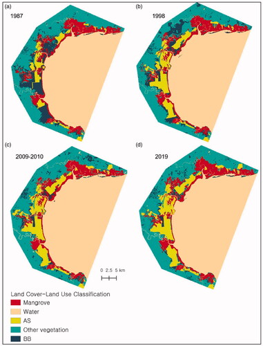
Figure 4. Mangrove gains and losses from 1987 to 2019 in Parita Bay.

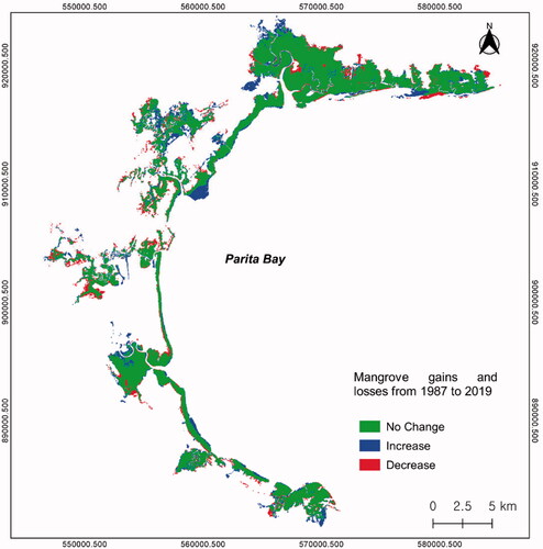
Table 2. Land use-cover change and rate of change in Parita Bay from 1987 to 2019.

No.		Area in hectares				Change in (%)				Rate of Change % per Year
	Class	1987	1998	2009–2010	2019	1987–1998	1998–2010	2010–2019	1987–2019	1987–1998	1998–2010	2010–2019	1987–2019
1	Mangrove	12,077.64	11,925.81	12,174.03	12,641.31	−1.26	2.08	3.84	4.67	−0.11	0.17	0.43	0.15
2	Water	64,824.75	64,754.1	64,824.66	64,372.5	−0.11	0.11	−0.70	−0.70	−0.01	0.01	−0.08	−0.02
3	AS	4776.57	9356.22	11,016.45	11,300.85	95.88	17.74	2.58	136.59	8.72	1.48	0.29	4.27
4	Other vegetation	27,171.45	25,649.1	26,627.4	27,194.58	−5.60	3.81	2.13	0.09	−0.51	0.32	0.24	0.00
5	Bare soil/Built-up	12,360.51	9525.69	6568.38	5701.68	−22.93	−31.05	−13.20	−53.87	−2.08	−2.59	−1.47	−1.68

The composite image from 2009–2010 is defined as 2010 for the change analysis.

Table 3. Matrix of change for each mangrove class from 1987 to 2019.

Class		1987–1998		1998–2009		2009–2019		1987–2019
From	To	Area (Ha)	%	Area (Ha)	%	Area (Ha)	%	Area (Ha)	%
Initial mangrove cover		12,077.64		11,925.81		12,174.03		12,077.64
1	1	10,625.76	87.98	10,303.65	86.40	10,877.40	89.35	10,475.82	86.74
1	2	208.62	1.73	212.40	1.78	89.82	0.74	243.72	2.02
1	3	157.86	1.31	152.37	1.28	210.78	1.73	453.51	3.75
1	4	719.64	5.96	1041.03	8.73	775.89	6.37	682.20	5.65
1	5	365.76	3.03	216.36	1.81	220.14	1.81	222.39	1.84
Loss (ha)—%		1451.88	12.02	1622.16	13.60	1296.63	10.65	1601.82	13.26
Final mangrove cover		11,925.81		12,174.03		12,641.31		12,641.31
1	1	10,625.76	87.98	10,303.65	86.40	10,877.40	89.35	10,475.82	86.74
2	1	225.36	1.87	319.32	2.68	401.58	3.30	668.52	5.54
3	1	51.12	0.42	79.11	0.66	28.62	0.24	26.01	0.22
4	1	609.93	5.05	829.89	6.96	1127.43	9.26	769.68	6.37
5	1	413.64	3.42	642.06	5.38	206.28	1.69	701.28	5.81
Gain (ha)—%		1300.05	10.76	1870.38	15.68	1763.91	14.49	2165.49	17.93
Net loss or gain			−1.26		2.08		3.84		4.67

Class 1 = Mangrove, 2 = Water, 3 = Aquaculture and Saltpans, 4 = Other Vegetation, and 5 = Bare Soil and Built-up.

Results from the mangrove cover matrix of change showed that 86.7% of the initial mangrove area remained unchanged throughout the entire study period; 13.26% of the initial mangrove area was lost and 5.65% had changed into Other Vegetation (AS (3.75%) and Others (Table 3)). Nevertheless, a 17.9% gain in new mangroves was derived from the conversion Other Vegetation (6.37%), BB (5.81%), and Water (5.54%). Moreover, the 136.6% increase in AS area was predominantly derived from the conversion of BB, contributing 114.1% or 5450.49 ha; the conversion of mangroves to AS contributed ∼ 9.5% or approximately 453.5 ha (Supplementary material, Table 3).

3.2. Temporal NDVI variability of mangroves and other vegetation

The 500 sampled NDVI values for mangrove coverage in our study area showed a left-skewed distribution (Figure 5(a)), indicating high or very high NDVI values (close to 1). In addition, the mean NDVI of mangroves in Parita Bay had increased over the 32 years, beginning with an initial decline during 1987–1998 (from 0.70 ± 0.07 to 0.67 ± 0.08) and increasing steeply in 2009 (0.81 ± 0.06); this was followed by a slight increase in 2019 (0.82 ± 0.06). This trend is consistent with the results of the mangrove land cover change analysis (Table 2).

Figure 5. (a) Boxplots of mangrove NDVI values from 1987 to 2019, (b) NDVI values for Other Vegetation sampled from 1987 to 2019. The data represents the 500 random samples of mangrove cover and other vegetation for the four time periods.

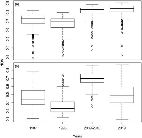
The distribution of Other Vegetation was irregular (Figure 5(b)) because it is composed of a number of vegetation types; this resulted in a wider NDVI range relative to that of the mangrove class. The mean NDVI for Other Vegetation during 1987, 1998, 2010, and 2019 was 0.46 ± 0.1, 0.36 ± 0.10, 0.70 ± 0.08, and 0.50 ± 0.13, respectively, with inconsistently skewed distributions in each period.

3.3. Mangroves changes in protected vs. unprotected areas

The annual mangrove coverage loss during 1987–1998 was slightly greater in protected (−0.17% yr⁻¹) relative to unprotected regions (−0.11% yr⁻¹) (Figure 6). However, mangroves in protected areas had later recovered at a rate of 0.56% yr⁻¹ from 1998 to 2010; this was followed by a decrease from 2010 to 2019 at a rate of −0.11% yr⁻¹. Mangroves in unprotected regions increased by 0.12% yr⁻¹ and 0.50% yr⁻¹ in the periods 1998–2010 and 2010–2019, respectively (Figure 6). Sarigua is one of two protected areas and the only protected area containing aquaculture activity (AS) in the study region. In Sarigua, AS cover had increased by 187.7% and 245.1% for the periods 1987–1998 and 1987–2019, respectively; these values were double those of unprotected regions at 85% and 123.7%, respectively (Tables 4 and 5). The mangrove losses and gains in each protected area were predominantly caused by changes in Other Vegetation (Supplementary material, Tables 8 and 9) based on the results of the matrix of change analysis.

Figure 6. The annual rate of change of protected versus unprotected areas. The last two bars on the graph indicate the accumulative results from 1987 to 2019.

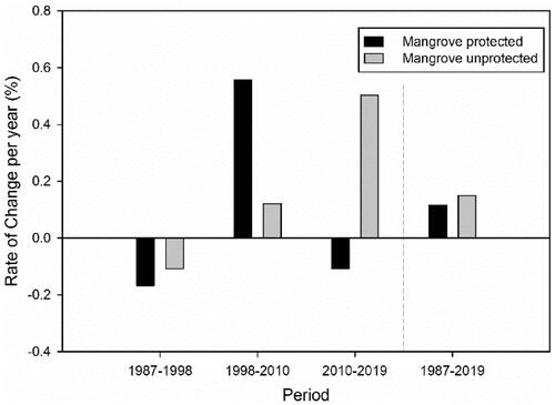
Table 4. Land use-cover loss and gains in the Cenegon de Mangle Wildlife Refuge and Sarigua National Park.

No.	Class	Total area in hectares				Change in %				Rate of change % per year
		1987	1998	2009	2019	1987–1998	1998–2009	2009–2019	1987–2019	1987–1998	1998–2009	2009–2019	1987–2019
1	Mangrove	1459.71	1432.89	1528.83	1514.07	−1.84	6.70	−0.97	3.72	−0.17	0.56	−0.11	0.12
2	Water	1291.77	1288.08	1278.81	1238.85	−0.29	−0.72	−3.12	−4.10	−0.03	−0.06	−0.35	−0.13
3	AS	506.79	1457.91	1812.33	1748.79	187.68	24.31	−3.51	245.07	17.06	2.03	−0.39	7.66
4	Other vegetation	316.8	388.17	523.89	579.06	22.53	34.96	10.53	82.78	2.05	2.91	1.17	2.59
5	Bare soil/Built-up	1939.32	947.34	370.53	433.62	−51.15	−60.89	17.03	−77.64	−4.65	−5.07	1.89	−2.43

Table 5. Land use-cover loss and gains in the unprotected area of the study region.

		Area in hectares				Change in %				Rate of Change % per Year
No.	Class	1987	1998	2009	2019	1987–1998	1998–2010	2010–2019	1987–2019	1987–1998	1998–2010	2010–2019	1987–2019
1	Mangrove	10,617.66	10,492.65	10,645.02	11,126.97	−1.2	1.5	4.5	4.8	−0.11	0.12	0.50	0.15
2	Water	63,532.62	63,465.66	63,545.4	63,133.29	−0.1	0.1	−0.6	−0.6	−0.01	0.01	−0.07	−0.02
3	AS	4269.78	7898.31	9204.12	9552.06	85.0	16.5	3.8	123.7	7.73	1.38	0.42	3.87
4	Other vegetation	26,854.65	25,260.93	26,103.51	26,615.52	−5.9	3.3	2.0	−0.9	−0.54	0.28	0.22	−0.03
5	Bare soil/Built-up	10,421.19	8578.35	6197.85	5268.06	−17.7	−27.8	−15.0	−49.4	−1.61	−2.31	−1.67	−1.55

3.4. Analysis of local climatic variables

3.4.1. Rainfall and temperature

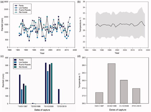
We used the accumulative rainfall and average temperature of the 3 months (90 days) prior to each satellite image capture to produce a comprehensive overview of each Landsat image (Galeano et al., 2017). Based on the one-way ANOVA test, we identified no significant differences in precipitation between Parita and Los Santos station (p = 0.477) in the north and between “Puerto Posada” and “Rio Hondo” stations (p = 0.607) in the south (Figure 7(a)). However, we identified a significant difference in precipitation between the south (Parita, Los Santos) and north (Puerto Posada, Rio Hondo) (maximum p = 0.005) (Supplementary material 2). The mean annual accumulative rainfall in Puerto Posada and Rio Hondo was higher than that of Parita and Los Santos over the 32 years. Similarly, the annual average daily maximum, mean, and minimum temperature in Parita Bay ranged from 31 to 34 °C, 27 to 29 °C, and 22 to 24 °C, respectively (Figure 7(b)). A cumulative rainfall of 185–377 mm occurred in the three months (90 days) prior to each image capture in 1987. We observed a decrease in precipitation during the next period (1998) at only 7.5 and 1.8 mm in Parita and Los Santos, respectively, and 0 mm in P. Posada and Rio Hondo. In contrast, the highest rainfall occurred during 2009, ranging from 424 to 532 mm. However, data for the 2019 image was only available from Parita station at 189.5 mm (Figure 7(c)). The average daily mean temperatures of the three months prior to image capture were 27.2, 29.1, 28.0, and 27.5 °C for 1987, 1998, 2009–2010, and 2019, respectively (Figure 7(d)).

Figure 7. (a) Annual accumulative rainfall in Parita Bay from January 1986 to December 2018. Each point represents the average accumulative daily rainfall calculated for each year at Parita, Los Santos, Puerto Posada, and Rio Hondo stations, (b) Minimum, mean, and maximum temperature in Parita Bay from 1986 to 2019, (c) Total precipitation amount of the 3 months prior to the date of capture for each Landsat image,d) Mean temperature in Parita Bay of the 3 months prior to the capture date of the Landsat images.

4. Discussion

4.1. Changes in mangrove area

Most studies across the globe have reported a net loss in mangrove forests with time (Brown et al. 2018; Gaw et al. 2018; Kanniah et al. 2015; Mondal et al. 2017; Polidoro et al. 2010; Tuholske et al. 2017). In contrast, our study identified an overall increase in mangrove area and mean NDVI in Parita Bay. Hamilton and Casey (2016) reported a global mangrove deforestation rate of −0.39% per year from 2000 to 2012; however, our results reflected an annual rate of increase of 0.17% during 1998–2009 and 0.43% yr⁻¹ in the following decade. In agreement, a number of recent studies also identified an expansion of mangrove forests, including a 5.5% increase in Fujian, China from 1995 to 2014 (Son et al. 2016; Godoy et al. 2018; Hsu and Lee 2018; Wang et al. 2018). In addition, mangroves were found to replace marshes over the past 60 years in the Gulf of Mexico (Bianchi et al. 2013).

Despite the overall increase in total mangrove area, 13.26% of the original mangrove cover (1601.82 ha) was predominantly replaced by Other Vegetation (682.20 ha) and AS (453.51 ha) throughout the 32 years. The observed decrease in mangrove cover from 1987 to 1998 also coincided with a 95.8% expansion of AS, which occurred at a significantly faster rate than the following two periods (17.74% and 2.58%, respectively). However, AS expansion had predominantly replaced BB (5450.49 ha) and Other Vegetation (804.15 ha), followed by mangroves (Tables 3 and 4). These findings are consistent with the results of previous studies, which showed that agriculture, aquaculture, and saltpans are the main anthropogenic drivers of global mangrove forest loss (Thomas et al. 2017). For example, India increased its aquaculture activities by 879% from 1988 to 2013, converting 0.63% of their mangrove area (Jayanthi et al. 2018). Similarly, aquaculture activity in Panama has rapidly expanded since the 1980s, and the country’s salt production increased from 2840 tons in 1987 to 7522 tons in 2017.

Simultaneously, we observed a 17.93% gain in mangrove area (2165.49 ha), resulting in an overall areal increase of 4.67%. This expansion was primarily due to the conversions of Other Vegetation (769.68 ha), BB (701.28 ha), and Water (668.52 ha), highlighting the impacts of natural regeneration and restoration programs on mangrove expansion. In general, mangrove forests are known to be highly resilient (Alongi 2008). Based on the visual inspection of remote sensing images, we identified a seaward expansion or seaward colonization of mangroves in some areas of the Parita Bay coast (Figure 4); this is likely due to the high accumulation of sediment through peat formation, demonstrating the mangroves high resilience (Lee et al. 2014).

The increase in mangrove area in our study site may also be due to reforestation and restoration activities. Reforestation-Afforestation programs are dominant factors influencing mangrove regrowth (Nursamsi and Komala 2017; Jayanthi et al. 2018). In Panama, these programs are either governmental or led by other sectors (e.g. NGOs, academics, and private business); they are also voluntary or mandatory (e.g. ecological compensation in national deforestation or forest clearance projects established by Environmental Impact Assessments). An example is the Project for Conservation and Resettlement of Threatened Mangrove Forests of the Pacific Panama, which was executed by the Panamanian government and funded by the International Tropical Timber Organization (ITTO) during 2004–2007. This program resulted in the reforestation of 500 hectares of mangrove forests in various sectors of the Pacific coast, including Parita Bay where 145 and 26 ha were reforested and restored in the provinces of Coclé and Herrera, respectively; this region is more specifically referred to as the Cenegon de Mangle Wildlife Refuge (ANAM 2009). Consequently, our results highlight the positive impacts of this reforestation program on mangrove expansion during 1998–2010 .

4.2. Variability and drivers of mangrove quality

In general, NDVI is related to canopy closure, leaf area index, aboveground biomass, and net primary productivity; it is also a good indicator of vegetation health. We therefore assessed changes in NDVI as a proxy for changes in mangrove forest quality (Sahebjalal and Dashtekian 2013; El-Gammal et al. 2014; Galeano et al. 2017; Tran and Fischer 2017; Zaitunah et al. 2018; Jin et al. 2019). The mean mangrove NDVI in Parita Bay was relatively high compared with other mangroves in tropical regions (Galeano et al. 2017; Rudiastuti et al. 2018). However, the net loss in mangrove area (−1.26%) during 1987–1998 was also accompanied by a decline in greenness (mean NDVI from 0.70 to 0.67, Figure 5(a)). This decline in NDVI also coincided with a drought period and an increase in temperature in the three months prior to the image capture (Figure 7(c,d)). NDVI is generally strongly related to precipitation regimes (Chamaille‐Jammes et al. 2006; Lee et al. 2019), and the ∼90 days of rainfall and temperature appear to influence the NDVI pattern in Parita Bay. In addition, 1997 and 1998 were significantly impacted by the El Niño-Southern Oscillation (ENSO) (Flores-Cárdenas et al. 2018), which likely enhanced the drought conditions in the study region. Therefore, rainfall, temperature, AS expansion, and their resulting interactions may have been the dominant cause for NDVI decline during 1987–1998; however, these factors are only some of the drivers involved in the gains and losses of mangroves in Parita Bay.

The classification results for the following two decades (1998–2019) revealed an increase in mangrove cover and NDVI. This recovery from forest loss highlights the stability and resilience of mangroves in Parita Bay due to conservation efforts, despite being located in the country’s driest region.

4.2. Protected vs natural areas in Parita Bay

Policies regarding forest protection and mangrove safeguarding have influenced the spatial variability of mangrove coverage across the world (Hsu and Lee 2018). In Panama, the principal mangrove forest regulations began in 1987 with the Resolution ADM-035-1987, which legalized the rational use and exploitation of mangrove forest products across the country. The Resolution JD-08-94 has been the main regulation for mangrove forest resources since 1994. In addition, the government have established the Wetland National Policy (MiAmbiente 2018), which includes an action plan for 2019–2023. This legal framework for the protection of wetlands in Panama could have mark the beginning of improved mangrove conservation; however, in recent days, not too much progress is observed. It is necessary to review and update regulatory frameworks in order to start implementing sort of conservation initiatives related with the protection and enhancement of these blue carbon ecosystems while benefitting local communities.

In this study, we detected irregular and unexpected trends when comparing protected and unprotected areas (Table 5). Both protected areas in the study region were established a number of years prior to our study period; however, they did not have a clear management plan. For example, 50% of the land in the Sarigua National Park was used for shrimp-breeding activities, and the rate of increase of aquacultural land use in Sarigua was more than double that of unprotected regions (245.1% versus 123.7%, respectively). Consequently, we observed a net loss in mangrove forest cover, and more than 157 hectares of mangrove forests were converted to AS during 1987–1998, despite the establishment of the conservation regulations. However, mangrove forests in protected areas during the next two decades (1998–2010) expanded at a rate of 0.56%, which was significantly higher than that of unprotected regions (0.12%). This rise coincided with the beginning of the reforestation program in the Pacific region of Panama developed in the Cenegon de Mangle Wild Refuge. Finally, our results inferred a net mangrove loss rate of −0.11% per year in protected areas and an expansion rate of 0.50% per year in unprotected areas during the last decade. Although it is inferred that Aquaculture activities have impacted on protected zone of Sarigua National Park (Ottinger et al. 2016; Jayanthi et al. 2018), the exact reason for the observed decrease in protected areas remains unclear; however, the results from the matrix of change analysis for both protected areas revealed a significant conversion of mangrove forests to Other Vegetation and BB (Table 4). Restoration programs and the conversion of mangroves to agricultural or grassland for cattle breeding are possible dominant causes of reduced mangrove coverage (León 2012).

In addition, the Sarigua National Park is exposed to high wind erosion (Cooke and Ranere 1992) and has one of highest soil degradation rates in the country (ANAM 2000). The region also experiences higher temperature, hyper salinity, and lower precipitation regimes compared to the rest of the country (MiAmbiente 2014). The mean annual accumulative rainfall in this study was lower near protected areas (Parita and Los Santos stations), inferring higher rain interception in unprotected regions over the past 32 years (Figure 7(a)). This suggests potentially higher degradation rates in protected areas without the influence of conservation activities. These findings are crucial for policy makers responsible for protected mangrove forests in Parita Bay and in other regions in Panama.

5. Conclusion

Mangrove coverage in the Parita Bay region has expanded over the last 32 years, showing high NDVI values. However, mangrove area and greenness experienced a net decrease from 1987 to 1998, which was likely influenced by both natural (e.g. rainfall and temperature) and anthropogenic factors (e.g. agriculture and the expansion of aquaculture and saltpan activities). Over the last decade, mangrove coverage had unexpectedly decreased in protected regions (the Cenegon de Mangle Wildlife Refuge and the Sarigua National Park) and increased in unprotected regions. Consequently, we suggest the implementation of a Management Effectiveness Evaluation in the protected areas of Parita Bay. Our study highlights the potential for mangrove reforestation and restoration in Parita Bay and provides useful information for policy makers to enhance the protection of mangrove ecosystems in the Pacific coast of Panama.

Authors’ contributions

Conceptualization, Y.B. and H.S.K.; data curation, Y.B.; formal analysis, Y.B.; writing-original draft preparation, Y.B.; methodology, K.K.; software, K.K.; supervision, H.S.K.; writing, review and editing, H.S.K.; funding acquisition, H.S.K.

Disclosure statement

No potential conflict of interest was reported by the author(s).

Additional information

Funding

This work was funded in part by the NIIED (National Institute for International Education of Korea) and Korea Forest Service [2018113B10-2020-BB01&2020185D10-2022-AA02].

References

- Afonso F, Félix PM, Chainho P, Heumüller JA, de Lima RF, Ribeiro F, Brito AC. 2021. Assessing ecosystem services in mangroves: insights from São Tomé Island (Central Africa). Front Environ Sci. 9:1.
- Alatorre LC, Sánchez-Carrillo S, Miramontes-Beltrán S, Medina RJ, Torres-Olave ME, Bravo LC, Wiebe LC, Granados A, Adams DK, Sánchez E, et al. 2016. Temporal changes of NDVI for qualitative environmental assessment of mangroves: shrimp farming impact on the health decline of the arid mangroves in the Gulf of California (1990–2010). J Arid Environ. 125:98–109.
- Alongi DM. 2008. Mangrove forests: resilience, protection from tsunamis, and responses to global climate change. Estuarine Coastal Shelf Sci. 76(1):1–13.
- Alongi DM. 2012. Carbon sequestration in mangrove forests. Carbon Manage. 3(3):313–322.
- ANAM. 2000. Primera Comunicacion Nacional sobre el cambio climatico ante el IPCC.109.
- ANAM. 2009. Informe Final de los Resultados del Proyecto Conservacion y Repoblacion de las areas amenazadas del Bosque de Manglar del Pacifico Panameno.78.
- ANAM and ARAP. 2013. Manglares de Panamá: importancia, mejores prácticas y regulaciones vigentes. Panamá: Editora Novo Art, S.A.:75.
- ANAM and UCCD. 2009. Atlas de las tierras secas y degradadas de panamá. 78.
- Bianchi TS, Allison MA, Zhao J, Li X, Comeaux RS, Feagin RA, Kulawardhana RW. 2013. Historical reconstruction of mangrove expansion in the Gulf of Mexico: linking climate change with carbon sequestration in coastal wetlands. Estuarine Coastal Shelf Sci. 119:7–16.
- Brown MI, Pearce T, Leon J, Sidle R, Wilson R. 2018. Using remote sensing and traditional ecological knowledge (TEK) to understand mangrove change on the Maroochy River, Queensland, Australia. Appl Geogr. 94:71–83.
- Castillo JAA, Apan AA, Maraseni TN, Salmo IIS. 2017. Estimation and mapping of above-ground biomass of mangrove forests and their replacement land uses in the Philippines using Sentinel imagery. ISPRS J Photogramm Remote Sens. 134:70–85.
- Chamaille‐Jammes S, Fritz H, Murindagomo F. 2006. Spatial patterns of the NDVI–rainfall relationship at the seasonal and interannual time scales in an African savanna. Int J Remote Sens. 27(23):5185–5200.
- Clevers J. 2009. In: Russell G. Congalton and Kass Green, editors. Assessing the accuracy of remotely sensed data—Principles and practices. Boca Raton (FL): CRC Press, Taylor & Francis Group; p. 183.
- Congedo L. 2016. Semi-automatic classification plugin documentation. Release. 4:29.
- Cooke R, Ranere AJ. 1992. Prehistoric human adaptations to the seasonally dry forests of Panama. World Archaeol. 24(1):114–133.
- CREHO-Ramsar. 2009. Inventario preliminar de los humedales continentales y costeros de Panamá.207.
- Donato DC, Kauffman JB, Murdiyarso D, Kurnianto S, Stidham M, Kanninen M. 2011. Mangroves among the most carbon-rich forests in the tropics. Nature Geosci. 4(5):293–297.
- Duke NC, Meynecke J-O, Dittmann S, Ellison AM, Anger K, Berger U, Cannicci S, Diele K, Ewel KC, Field CD, et al. 2007. A world without mangroves? Science. 317(5834):41–42.
- El-Gammal M, Ali R, Samra RA. 2014. NDVI threshold classification for detecting vegetation cover in Damietta governorate, Egypt. J Am Sci. 10:108–113.
- FAO. 2015. Evaluation de los Recursos Forestales Mundiales 2015 - Panama.104.
- Flores-Cárdenas F, Millán-Aguilar O, Díaz-Lara L, Rodríguez-Arredondo L, Hurtado-Oliva MÁ, Manzano-Sarabia M. 2018. Trends in the normalized difference vegetation index for mangrove areas in northwestern Mexico. J Coast Res. 344:877–882.
- Friess DA. 2016. Mangrove forests. Curr Biol. 26(16):R746–R748.
- Galeano A, Urrego LE, Botero V, Bernal G. 2017. Mangrove resilience to climate extreme events in a Colombian Caribbean Island. Wetlands Ecol Manage. 25(6):743–760.
- Gaw LY, Linkie M, Friess DA. 2018. Mangrove forest dynamics in Tanintharyi, Myanmar from 1989–2014, and the role of future economic and political developments. Singapore J Trop Geogr. 39(2):224–243.
- Ghosh MK, Pal J, Roy PK. 2017. How memory regulates drug resistant pathogenic bacteria? A mathematical study. Int J Appl Comput Math. 3(S1):747–773.
- Gilman EL, Ellison J, Duke NC, Field C. 2008. Threats to mangroves from climate change and adaptation options: a review. Aquat Bot. 89(2):237–250.
- Gilman EL, Ellison J, Jungblut V, Van Lavieren H, Wilson L, Areki F, Brighouse G, Bungitak J, Dus E, Henry M, et al. 2006. Adapting to Pacific Island mangrove responses to sea level rise and climate change. Clim Res. 32:161–176.
- Giri C, Ochieng E, Tieszen LL, Zhu Z, Singh A, Loveland T, Masek J, Duke N. 2011. Status and distribution of mangrove forests of the world using earth observation satellite data. Global Ecol Biogeogr. 20(1):154–159.
- Godoy MDP, de Andrade Meireles AJ, de Lacerda LD. 2018. Mangrove response to land use change in estuaries along the semiarid coast of Ceará, Brazil. J Coast Res. 34(3):524–533.
- Hamilton SE, Casey D. 2016. Creation of a high spatio‐temporal resolution global database of continuous mangrove forest cover for the 21st century (CGMFC‐21). Global Ecol Biogeogr. 25(6):729–738.
- Hsu L-C, Lee C-T. 2018. The current extent and historical expansion of mangroves in the Kuantu Nature Reserve, North Taiwan. J Coast Res. 34:360–372.
- Islam MM, Borgqvist H, Kumar L. 2019. Monitoring Mangrove forest landcover changes in the coastline of Bangladesh from 1976 to 2015. Geocarto Int. 34(13):1458–1476.
- Jayanthi M, Thirumurthy S, Muralidhar M, Ravichandran P. 2018. Impact of shrimp aquaculture development on important ecosystems in India. Global Environ Change. 52:10–21.
- Jayanthi M, Thirumurthy S, Nagaraj G, Muralidhar M, Ravichandran P. 2018. Spatial and temporal changes in mangrove cover across the protected and unprotected forests of India. Estuarine Coastal Shelf Sci. 213:81–91.
- Jin E-J, Yoon J-H, Bae E-J, Choi M-S. 2019. Photosynthesis and chlorophyll fluorescence of evergreen hardwoods by drying stress. Korean J Agric For Meteorol. 21:196–207.
- Kamruzzaman M, Basak K, Paul SK, Ahmed S, Osawa A. 2019. Litterfall production, decomposition and nutrient accumulation in Sundarbans mangrove forests, Bangladesh. For Sci Technol. 15(1):24–32.
- Kamruzzaman M, Paul SK, Ahmed S, Azad MS, Osawa A. 2019. Phenology and litterfall production of Bruguiera sexangula (Lour.) Poir. in the Sundarbans mangrove forests. Bangladesh. For Sci Technol. 15(3):165–172.
- Kanniah KD, Sheikhi A, Cracknell AP, Goh HC, Tan KP, Ho CS, Rasli FN. 2015. Satellite images for monitoring mangrove cover changes in a fast growing economic region in southern Peninsular Malaysia. Remote Sensing. 7(11):14360–14385.
- Kauffman JB, Donato DC. 2012. Protocols for the measurement, monitoring and reporting of structure, biomass, and carbon stocks in mangrove forests. Working Paper 86. Center for International Forestry Research.
- Kuenzer C, Bluemel A, Gebhardt S, Quoc TV, Dech S. 2011. Remote sensing of mangrove ecosystems: A review. Remote Sensing. 3(5):878–928.
- Lee EJ, Piao D, Song C, Kim J, Lim C-H, Kim E, Moon J, Kafatos M, Lamchin M, Jeon SW, et al. 2019. Assessing environmentally sensitive land to desertification using MEDALUS method in Mongolia. For Sci Technol. 15(4):210–220.
- Lee SY, Primavera JH, Dahdouh-Guebas F, McKee K, Bosire JO, Cannicci S, Diele K, Fromard F, Koedam N, Marchand C, et al. 2014. Ecological role and services of tropical mangrove ecosystems: a reassessment. Global Ecol Biogeogr. 23(7):726–743.
- León IRD. 2012. Línea Base: diagnóstico biofísico, socioeconómico y potencial energético de la Cuenca del Río Parita [Baseline: biophysical, socioeconomic and energy potential diagnosis of the Parita River Basin]. Ancón (Albrook): Nacional del Ambiente.
- McGowan T, Cunningham SL, Guzmán HM, Mair JM, Guevara JM, Betts T. 2010. Mangrove forest composition and structure in Las Perlas Archipelago, Pacific Panama. Rev Biol Trop. 58(3):857–869.
- MiAmbiente. 2014. Sarigua; Un ejemplo de recuperación de suelos para el mundo. Ministerio de Ambiente. 19.
- MiAmbiente. 2018. Politica Nacional de Humedales de la Republica de Panama. Ministerio de Ambiente. 73.
- Mondal P, Trzaska S, De Sherbinin A. 2017. Landsat-derived estimates of mangrove extents in the Sierra Leone coastal landscape complex during 1990–2016. Sensors. 18(2):12.
- Nursamsi I, Komala WR. 2017. Assessment of the successfulness of mangrove plantation program through the use of open source software and freely available satellite. Nusantara Biosci. 9(3):251–259.
- Ottinger M, Clauss K, Kuenzer C. 2016. Aquaculture: relevance, distribution, impacts and spatial assessments–a review. Ocean & Coastal Management. 119:244–266.
- Polidoro BA, Carpenter KE, Collins L, Duke NC, Ellison AM, Ellison JC, Farnsworth EJ, Fernando ES, Kathiresan K, Koedam NE, et al. 2010. The loss of species: mangrove extinction risk and geographic areas of global concern. PLoS One. 5(4):e10095.
- Rahman MTU, Tabassum F, Rasheduzzaman M, Saba H, Sarkar L, Ferdous J, Uddin SZ, Islam AZ. 2017. Temporal dynamics of land use/land cover change and its prediction using CA-ANN model for southwestern coastal Bangladesh. Environ Monit Assess. 189(11):565.
- Rioja-Nieto R, Barrera-Falcón E, Torres-Irineo E, Mendoza-González G, Cuervo-Robayo AP. 2017. Environmental drivers of decadal change of a mangrove forest in the North coast of the Yucatan peninsula. J Coast Conserv. 21(1):167–175.
- Rouse J, Haas R, Schell J, Deering D. 1974. Monitoring vegetation systems in the Great Plains with ERTS. NASA Spec Publ. 351:309.
- Rudiastuti AW, Yuwono DM, Hartini S. 2018. Mangrove mapping using SPOT 6 at East Lombok Indonesia. Proceedings of the IOP Conference Series: Earth and Environmental Science. IOP Publishing.
- Sahebjalal E, Dashtekian K. 2013. Analysis of land use-land covers changes using normalized difference vegetation index (NDVI) differencing and classification methods. Afr J Agric Res. 8:4614–4622.
- Servino RN, de Oliveira Gomes LE, Bernardino AF. 2018. Extreme weather impacts on tropical mangrove forests in the Eastern Brazil Marine Ecoregion. Sci Total Environ. 628–629:233–240.
- Seto KC, Fragkias M. 2007. Mangrove conversion and aquaculture development in Vietnam: a remote sensing-based approach for evaluating the Ramsar Convention on Wetlands. Global Environ Change. 17(3-4):486–500.
- Son NT, Thanh BX, Da CT. 2016. Monitoring mangrove forest changes from multi-temporal Landsat data in Can Gio Biosphere Reserve, Vietnam. Wetlands. 36(3):565–576.
- Spalding M. 2010. World atlas of mangroves. London: Routledge.
- Thomas N, Lucas R, Bunting P, Hardy A, Rosenqvist A, Simard M. 2017. Distribution and drivers of global mangrove forest change, 1996–2010. PLoS One. 12:e0179302.
- Tilahun A, Teferie B. 2015. Accuracy assessment of land use land cover classification using Google Earth. AJEP. 4(4):193–198.
- Tran LX, Fischer A. 2017. Spatiotemporal changes and fragmentation of mangroves and its effects on fish diversity in Ca Mau Province (Vietnam). J Coast Conserv. 21(3):355–368.
- Tuholske C, Tane Z, López-Carr D, Roberts D, Cassels S. 2017. Thirty years of land use/cover change in the Caribbean: assessing the relationship between urbanization and mangrove loss in Roatán, Honduras. Appl Geogr. 88:84–93.
- UNESCO. 2008. Balance hídrico superficial de Panamá, Periodo 1971-2002.135.
- USGS. 2017. Landsat 8 Level 1 Data Format Control Book 11.26.
- USGS. 2018. Landsat 4-7 Surface Reflectance (Ledaps). 32.
- Valderrama-Landeros L, Flores-de-Santiago F, Kovacs J, Flores-Verdugo F. 2017. An assessment of commonly employed satellite-based remote sensors for mapping mangrove species in Mexico using an NDVI-based classification scheme. Environ Monit Assess. 190(1):23.
- Wang M, Cao W, Guan Q, Wu G, Wang F. 2018. Assessing changes of mangrove forest in a coastal region of southeast China using multi-temporal satellite images. Estuarine Coastal Shelf Sci. 207:283–292.
- Wulder MA, Franklin SE. 2012. Remote sensing of forest environments: concepts and case studies. Boston (MA): Springer Science & Business Media.
- Yengoh GT, Dent D, Olsson L, Tengberg AE, Tucker CJ. III 2015. Use of the Normalized Difference Vegetation Index (NDVI) to assess land degradation at multiple scales: current status, future trends, and practical considerations. Boston (MA): Springer.
- Yoo BH, Kim KS, Lee J. 2019. The use of MODIS atmospheric products to estimate cooling degree days at weather stations in South and North Korea. Korean J Agric For Meteorol. 21:97–109.
- Young NE, Anderson RS, Chignell SM, Vorster AG, Lawrence R, Evangelista PH. 2017. A survival guide to Landsat preprocessing. Ecology. 98(4):920–932.
- Zaitunah A, Ahmad A, Safitri R. 2018. Normalized difference vegetation index (ndvi) analysis for land cover types using landsat 8 oli in besitang watershed, Indonesia. Proceedings of the IOP Conference Series: Earth and Environmental Science. IOP Publishing.