Remote sensing based forest canopy opening and their spatial representation

Abstract

The use of remote sensing in natural resource management is an easily accessible input for obtaining detailed information on the ground and landscape. There is a wide range of procedures to analyze the forest canopy through satellite images. The purpose of this work is to obtain a map of forest opening with remote sensing by relating several vegetation indices, Kauth-Thomas transformation and texture filters, to a Landsat 8OLI image. A factor analysis was made to evaluate the contribution of these variable to identify the opening of the forest cover, yielding a σ2 = 76%. The results show that the Modified Soil Adjusted Vegetation Index (MSAVI), Soil Adjusted Vegetation Index (SAVI), and brightness factor have the best correlation (0.225–0.216 component coefficient). The resulting model was reclassified into five categories of forest opening and associated with land use data from the National Institute of Statistics and Geography (INEGI-México). Thus, 95% of human settlements have a canopy opening between medium and very high, the crops areas 72%, and the low deciduous forest with secondary shrub vegetation 100% of the opening. Coniferous and mixed forests have a low to very low canopy opening 46% and 55%, respectively of their surface. The forests with secondary vegetation, both shrub and arboreal, present greater openness than the same forests in the primary state. Verification of the spatial representation data of canopy opening was made by comparing 94 hemispheric photographs with 94 sites located in open areas obtaining an r = 0.57. This work offers a simple and straightforward methodology, easily replicable in different types of vegetation using free satellite imagery. Hence, it is a helpful tool for decision-makers when considering the general status of conservation of forest systems and their spatial distribution.

Keywords:

• Remote sensing
• canopy opening
• vegetation indexes
• Tasseled Cap

1. Introduction

The importance of forests can be evaluated by the occupied area, their distribution, and the goods and services provided (Wulder 1998; Shvidenko et al. 2005). Changes in forest areas are mainly due to agricultural expansion and infrastructure development. Both processes are associated with the massive loss of biological diversity (Fuller 2006). Anthropic activities such as deforestation, firewood extraction, agricultural activities, among others, are serious threats to forest areas, due to the modification or elimination of physical, chemical, and biological processes (Norman 1984; Poyatos et al. 2003).

The grade of conservation of the vegetation cover is relevant because it is related to processes occurring from the highest part of the canopy to the ground. For instance, the amount of precipitation passing through trees provides elements to recognize forests as soil protection agents, erosion mitigations (Dunkerley 2020), and aquifer rechargers (Bishop et al. 2006). In forests, the physical and chemical processes are strongly linked to the density of the vegetation cover, since it regulates the entry of light, water, and wind from the top of the trees to the ground (Percy 1989). The cover density can be related to the type of tree association, the type of species composing them, their spatial distribution, leaves arrangement, climate, and phenology (as in the case of deciduous species) (Alkama and Cescatti 2016).

One of the most widely used indirect methods for measuring cover density, specifically canopy opening, are the hemispherical photographs. However, even though these data provide specific information that can be extrapolated, they are impractical in large areas, due to economic issues and time efficiency, involving a wide photographic coverage in large forested areas (Welles and Cohen 1996). Therefore, a synoptic view such as that from satellite imagery is a good choice for larger areas or regional studies (Potapov et al. 2011). Satellite images, obtained through remote sensors, collect electromagnetic information from a distance without being physically at the site, allowing to recognize vegetation cover, meteorological systems, oceanographic and atmospheric features, geological characteristics, among others (Schanda 2012). The data detection capacity of a remote sensor depends on both the platform on which they are mounted and the spectral resolution defined by the number of bands (Jones and Vaughan 2010). The knowledge of the reflective response of different targets makes it possible to recognize a variety of patterns in the image. (Schroeder et al. 2006).

One of the main applications of satellite images in the biogeographical field is the utilization of vegetation indices. Vegetation cover has a particular spectral response in the red and infrared bands, which makes it possible an easy detection. Important information such as greenness and humidity in the vegetation, plant density, and bare soil detection can be inferred (Bannari et al. 1995), which can be useful to discriminate areas with and without vegetation (Meléndez Pastor et al. 2009). The use of satellite images for mapping and monitoring of vegetation has been a long term used tool due to its accessibility and availability in different spectral and spatial resolutions (Zhu and Liu 2014), allowing multi-temporal information at various scales (Muñoz 2013).

This work makes use of satellite images, for evaluating the relative importance of various vegetation indices, and variables such as texture, brightness, greenness, and wetness, to identifying and recognizing the opening of the canopy. Additionally, factor analysis is used to find the best-matching variables associated with the identification of the opening of the canopy cover which will be represented by map algebra. Therefore, by identifying the opening level of the forest cover, the state of conservation or alteration of the study area can be inferred. Finally, to differentiate by type of vegetation and its level of opening, the cartography of land use and the vegetal formations of series VI of the National Institute of Statistic and Geography (INEGI 2017b) have been used as an ancillary information. The present study is a methodological approach, easily replicable in different forest ecosystems with the use of freely accessible inputs. The methods used here are based on the spectral response captured by satellite imagery and the application of different indices allowing the identification of the opening in the forest cover.

2. Methods

2.1. Study area

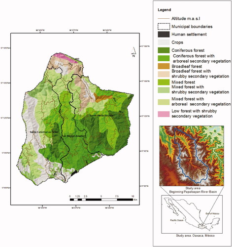
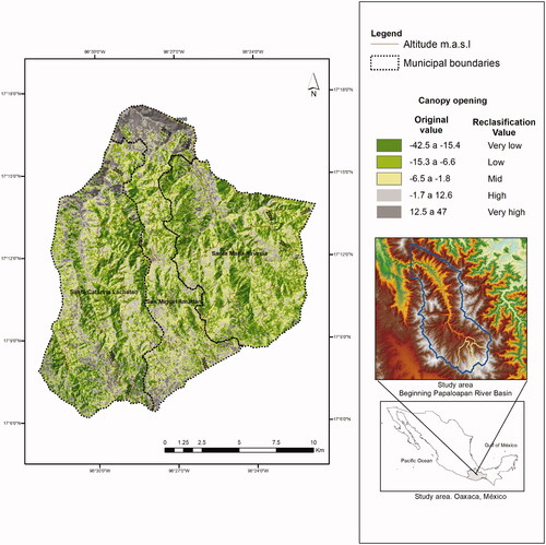
The study area includes three municipalities: San Miguel Amatlán, Santa Catarina Lachatao and Santa María Yavesía, which belong to the District of Ixtlán, located in the Sierra Norte or Sierra Juárez, within the Sierra Madre del Sur, in the Mexican state of Oaxaca. Its extreme coordinates are: 17.29° and 17.10° north latitude and 96.53° and 96.35° west longitude (INEGI 2005). It comprehends 24,979 ha, of which 88% are covered by temperate forests of different types, such as coniferous, broadleaf, and mixed forests in different states of conservation (INEGI 2017b) (Figure 1). It is characterized by having mainly forest land use with 81% forests, 17% occupied by crops, and 1.3% by human settlements. There is an altitude gradient that ranges between 1600 and 3400 m a. s. l., which produces a very rugged relief. The average annual temperature is 10 °C in the highest parts and 20 °C in the lowest ones. The hottest months are April and May, while the coldest months are November, December, and January (INEGI 2005). Annual precipitation is greater than 1200 mm per year, descending to 800 mm, at lower altitudes, and having the rainiest period from May to September. The three municipalities have a total population of 2798 inhabitants (INEGI 2010), distributed in 8 settlements within the area.

Figure 1. Location of the study area, types of vegetation, land use and its conservation status according to the INEGI classification (series VI, 2017), modified for this study. Reference: Land use from National Institute of Statistic and Geography, 2017.

2.2. Estimation of the Forest canopy opening

To analyze the possibility of recognizing canopy openings in the vegetation cover, a free access Landsat 8-OLI image was used (https://ers.cr.usgs.gov) corresponding to Path 24/Row 48, dated 19 March 2013 (dry season). Visible and infrared bands (2–7) with spatial resolution of 30 m and the panchromatic band (8) with a spatial resolution of 15 m were used. The following vegetation indices were applied: Difference Vegetation Index-DVI (Tucker 1979), Normalized Difference Vegetation Index-NDVI (Rouse 1974), Soil Adjusted Vegetation Index-SAVI (Huete 1988), Vegetation Index Adjusted by Modified Soil-MSAVI (Qi et al. 1993, 1994), Moisture Stress Index-MSI (Hunt and Rock 1989) (Supplemental Appendix 1), in addition to Tasseled Cap (Kauth–Thomas Transformation) and texture analysis. To obtain each of these products, various processes were carried out, and are described below. Later, these values were statistically correlated with the opening of the forest canopy.

To have an estimation of the distribution of plant communities and transformed regions in the study area, the information generated by the INEGI (2017b) was used, which describes the different types of forests grouped according to their conservation status, including secondary vegetation. The knowledge of the land use of the study area helps to have a reference and to recognizing spectral and spatial differences in the satellite images.

2.3. Tasseled Cap analysis (Kauth–Thomas)

To obtain the brightness, greenness, and wetness characteristics of the forest cover in the satellite image, a Tasseled Cap (TC) analysis was applied. This transformation consists of a new set of bands generated by linear combinations of all bands, useful in vegetation mapping. This analysis was proposed by Kauth and Thomas in 1976 and is based on the vegetation phenology. It spatially transforms vegetation data into three linear combinations of spectral bands with specific weights (or eigenvectors). These new bands are known as brightness, greenness, and wetness (Jones and Vaughan 2010).

The brightness is associated with bare soil, thus high brightness values, can be an indicator of a change toward uncovered or sparsely vegetated areas. Greenness is related to the presence of chlorophyll and photosynthetic activity, changes detected in this band are related to the increase or decrease of vegetation. Wetness can be an indicator of the density of vegetation and soil moisture, so, low humidity values would be an indicator of a senescent vegetation or under water stress (Rahman and Mesev 2019).

TC analysis for LANDSAT imagery (MMS, TM and ETM) is well established. Each sensor possesses its own linear combinations with their specific eigenvectors. However, this study focuses on the analysis of the Landsat8-OLI sensor and a proper TC analysis has not yet been established. Most common software for processing satellite images, such as Erdas, Envi, or ArcGis, does have not a particular TC algorithm for Landsat8-OLI (Erdas Help, Envi Help, Arcgis Help). Nonetheless, Baig et al. (2014), proposed a set of eigenvectors for transforming Landsat 8 image. First, the digital values were converted to radiance values applying the method suggested by the National Aeronautics and Space Administration (NASA-USGS 2019). Whit this information map algebra method was used to perform the TC analysis (1) $$TC=(B2*C_{\text{i}}+B3*C_{\text{i}}*B4*C_{\text{i}}+B5*C_{\text{i}}+B6*C_{\text{i}}+B7*C_{\text{i}})$$(1) where TC = Tasseled Cap, B2 = Band 2 (0.45–0.51 μm), B3 = Band 3 (0.53–0.59 μm), B4 = Band 4 (0.63–0.67 μm), B5 = Band 5 (0.85–0.88 μm), B6 = Band 6 (1.57–1.65 μm), B7 = Band 7 (2.11–2.29 μm), C = Coefficient, i = coefficient value for each component based on Baig et al. (2014).

2.4. Hemispherical photographs

It is one of the most widely used indirect methods for measuring cover density, specifically canopy opening. It provides local and specific information and, although it can be extrapolated, is impractical in large areas because is expensive and time consuming (Welles and Cohen 1996). In this study, 94 hemispheric photographs were taken in 2013 with a digital camera Canon EOS Rebel equipped with a SIGMA wide angle lens or “fish-eye.” Hemispherical photographs were processed with the free access program GLA (Gap Light Analyzer) (Frazer et al. 1999), and represent the percentage of canopy opening.

2.5. Texture analysis

It is a powerful statistical kernel-based tool for assessing spatial homogeneity. The texture analysis of satellite imagery involves identification and measurement of patterns, shapes, and sizes. It is based on the connectivity of the pixels containing spatial information on the tonal variations of each band. Even though it has not been widely used as spatial analysis, nowadays, its application is increasing in studies of land use classification, modeling habitats, and vegetation structure (Coburn and Roberts 2004). Here, the texture analysis was performed for identifying changes in different spatial patterns of tone and roughness in the vegetation structure in the green and infrared bands because of spectral reflectance (Franklin et al. 2000; Coburn and Roberts 2004; Clark and Hardegree 2005); which can be classified as: fine or smooth, thick, rough, regular and irregular (Lee et al. 2005; Rodríguez 2008).

Texture filters with, kernel of 9 × 9 and 11 × 11 were used to determine the most suitable in identifying the opening of the canopy (Anaya et al. 2008; Culbert et al. 2009). Some studies consider that smaller windows (3 × 3 or 5 × 5) are inaccurate due to the lack of significant changes in the window (for very homogeneous areas) (Chica-Olmo and Abarca-Hernández 2000). In this study, the co-occurrence method of texture analysis was applied because it highlights the difference in gray tones (ENVI 5.0. Exelisvis, 2012). The co-occurrence method returns derived products such as mean ($\overline{\text{x}}$), variance (S²), homogeneity (r_j), contrast (F), dissimilarity (D), entropy (H), second moment (g₂), and correlation (ρ) (Haralick et al. 1973); (ENVI Help, version 5.0).

A total of 32 texture measurements were applied, eight for the green band and eight for the near-infrared band, both with the mentioned window sizes. To compare the results of the texture filters with the status of opening of the canopy, 188 sampling points were used, 94 correspond to hemispheric photographs taken randomly in previous studies of forest inventories in 2013 and relate to the different types of forest located in the study area and 94 random points as a balance to hemispheric photographs, these sites correspond to areas without vegetation cover or with high canopy opening. Due to terrain topography, there are places where hemispherical photographs cannot be taken the remaining 94 randomly distributed sampling points, were selected through visual recognition in the Landsat image and INEGÍs land use map (INEGI 2017b). These points were identified as sites of maximum opening. To compare the values of the sampling sites with the 32 texture filters it was necessary to normalize them. Finally, a bi-dimensional scatterplot analysis allowed the identification of the highest correlation between these values and the percentage of vegetation cover opening.

2.6. Spatial representation of the opening of the vegetation cover

To obtain the spatial representation of the forest canopy opening, recognized from the satellite image, a factor analysis was made (Hair et al. 1999). The variables used in the analysis were: brightness, greenness, and wetness (derived from TC), the five vegetation indices: DVI, NDVI, SAVI, MSAVI, and MSI (Supplemental Appendix 1), the texture measurement and the slope, which is an important element related to deforestation (Mas et al. 2002). Terrain slope data were obtained from the Mexican Continuous of Elevations (CEM-INEGI 3.0, INEGI 2017a). Statistical analysis was performed with the SPSS version 18 program (PAWS Statistics 21 2010) accounting for a total of 1,091,470 records. With the results of the factor analysis, the spatial representation of the opening of forest vegetation cover was elaborated employing the map algebra method (ArcGis 10.2.2), factor analysis equation, is represented as follows: (2) $$\mathit{OVC}=\sum (B_{1\text{ci}}+G_{2\text{ci}}+H_{3\text{ci}}+DV{I}_{4\text{ci}}+\mathit{NDV}{I}_{5\text{ci}}+\mathit{SAV}{I}_{6\text{ci}}+\mathit{MSAV}{I}_{7\text{ci}}+MS{I}_{8\text{ci}}+T_{9\text{ci}}+S_{10\text{ci}})$$(2) where,

OVC = Opening of the vegetation cover, B = Brightness, G = Greenness, H = Wetness, DVI, NDVI, SAVI, MSAVI, MSI, T = Texture, S = Slope, c = Coefficient, i = coefficient value for each variable (obtained from the coefficient matrix).

To identify the grade of similarity between these variables, a simple linear correlation analysis was performed by considering the 188 sampling points containing the percentage of opening data derived from hemispheric photographs and the resulting map of the opening of vegetation cover, without reclassification (Pardo and Ruiz 2002). The result of the spatial representation of the vegetation cover opening, was reclassified into five categories using the Jenks method, consisting, in grouping similar values and maximizing the differences between classes (Jenks 1967; Buzai et al. 2019). This reclassification was done, for optimally organizing the information (Harvey and Rodrigo 1983). Finally, this result was merged with the land use and vegetation map to have a reference of the behavior of the forest cover opening by vegetation type (INEGI 2017b).

3. Results

3.1. Tasseled Cap

The TC analysis generates brightness, greenness, and wetness new bands of the study area coverage. Figure 2 shows the interval of values of these variables. The brightness component ranges from 0 to 563. It is apparent that 35% of the values are equal to 0, while 65% corresponds to the remainder. Values over 150 are related to areas with low forest canopy covers, such as crops and human settlements, broadleaf forest, and shrubby secondary broadleaf forest.

Figure 2. Result of the Tasseled cap analysis with minimum and maximum values for brightness, greenness, and humidity and mean and standard deviation values for brightness, greenness and humidity. CF: coniferous forest; MF: mixed forest; BF: broadleaf forest; CFSArb: coniferous forest with arboreal secondary vegetation; MFSArb: mixed forest with arboreal secondary vegetation; MFShr: mixed forest with shrubby secondary vegetation; BFShr: broadleaf forest with secondary shrub vegetation; LFShr: low forest with secondary shrub vegetation; Crops: crops; HS: human settlement.

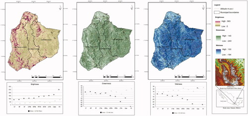
The values of the greenness component range from −243 to 140. Negative values correspond to open areas or with low vegetation density. Positive values correspond to areas with high vegetation coverage, representing 86%. Coniferous forest and mixed forest, including arboreal secondary vegetation, have the highest greenness values, markedly contrasting with crops and broadleaf forest with shrubby secondary vegetation.

The range of values of the wetness component spans from −194 to 153. Values below −22 correspond to areas with low or no-canopy coverage (15%), located in zones of crops or of human settlements. Values between −22 to 0 can be associated to broadleaf forests. Positive wetness values correspond to mixed and coniferous forests (66%), which incidentally have the highest values, coinciding with the high values of greenness. Crops and primary and secondary shrubby broadleaf forest are identified as zones with low wetness, low greenness and high brightness values due to the scarce presence of canopy (Figure 2).

In Figure 2 also shows the graphic representation of average of the mean and standard deviation values by TC and land use. In the brightness band the highest mean and standard deviation values correspond to human settlements and crops areas (greater opening), and in the same way to low forest and broadleaf forest with shrubby secondary vegetation. Coniferous and mixed forest have mean values between 85 and 87, while the rest of the forests are over 105. The negative values of greenness correspond to open areas such as human settlements, crops, secondary broadleaf forest shrubby, and shrubby secondary low forest. Coniferous and mixed forests have mean values above 20, while secondary coniferous arboreal forests and broadleaf forests have mean values lower than the previous ones. Mean values for wetness are negative in almost all types of land use, except for coniferous and mixed forests, that are identified with higher wetness. The standard deviation is low in all land use types, possibly caused by the variability and heterogeneity of species present in the study area, which might affect the spatial resolution of the sensor when trying to discriminate this diversity per pixel.

3.2. Vegetation indices

Difference Vegetation Index (DVI) values fluctuate between −169 to 195. Negative values, represent 69% of the data and correspond to areas occupied by coniferous and mixed forest. Values above 0 belong to crops areas and human settlements. All the forested areas show negative values, while secondary coniferous, mixed and shrubby broadleaf forests have values close to 0, due to the low density of the forest canopy.

Normalized Vegetation Index (NDVI) values range from −1 to 0.5. Negative values (37%) correspond to areas with low or no forested cover. The rest of the image contains values from 0 to 0.5, and represent homogeneous and photosynthetically active areas that can be associated with coniferous and mixed forests with the highest mean values, while crops areas and secondary broadleaf forest are characterized by having low index values. The broadleaf, secondary arboreal coniferous and mixed secondary arboreal forests have the same spectral response with mean values of 0.03.

The Soil Adjusted Vegetation Index (SAVI) shows values between −0.80 and 1.49. Negative values represent 60% of the coverage and correspond to forest. Positive values can be identified with opening areas. Coniferous and mixed forests have the lowest values, while the broadleaf forests and the coniferous and mixed secondary arboreal forests have values close to 0, this effect is due to the correction factor of SAVI that highlights the differences between bare soil and vegetated areas.

The Modified Soil Adjusted Vegetation Index (MSAVI) values range from −2 to 1. Like SAVI, the negative values comprehend the 60% of the data and correspond to coniferous and mixed forest areas. The rest of the data, with positive values, correspond to areas with low vegetation cover. This index has the same behavior as the SAVI since both were designed to differentiate bare soil from vegetated areas.

Finally, the Moisture Stress Index (MSI), ranged from 0.4 to 1.5. MSI Values < 0.80 represent the most homogeneous and best conserved forest areas, with the wetness strongly associated to the highest precipitation data, in the study area. In the MSI, the highest values correspond to human settlements, crops and broadleaf forests, areas under water stress are clearly identified in the broadleaf, mixed and secondary forest. The coniferous forest has the lowest values or the least water stress (Figure 3) (Supplemental Appendix 1).

Figure 3. Result of vegetation indices with minimum and maximum values for DVI, NDVI, SAVI, MSAVI and MSI and Mean and standard deviation values for the applied vegetation indices. CF: coniferous forest; MF: mixed forest; BF: broadleaf forest; CFSArb: coniferous forest with arboreal secondary vegetation; MFSArb: mixed forest with arboreal secondary vegetation; MFShr: mixed forest with shrubby secondary vegetation; BFShr: broadleaf forest with secondary shrub vegetation; LFShr: low forest with secondary shrub vegetation; Crops: crops; HS: human settlement.

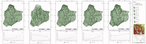
Figure 3 also shows the graphic representation of average shows the average of the mean and standard deviation values by vegetation index and land use. DVI has negative mean values in most forest coverage: primary and secondary mixed forest, primary and secondary coniferous forest, and broadleaf forest. Positive values correspond to low-density or opened areas such as human settlements, crops, secondary shrubby broadleaf forest, and secondary shrubby lowland forest. For NDVI, results were as expected, that is, the mean positive values correspond to primary coniferous, mixed, broad-leaved forest and forests with secondary coniferous and mixed arboreal vegetation. The mixed forest with secondary shrub vegetation has a slightly decrement in the NDVI values due to the lower density in this type of secondary vegetation. Negative values can be associated with crops, shrubby secondary broadleaf forest, human settlement, and shrubby secondary lowland forest.

Mean values of SAVI and MSAVI are similar since both indices have a correction factor accounting for soil presence an influence. In both indices, the mean negative values correspond to the best conserved secondary forest cover with arboreal vegetation. Positive values correspond to low-density land uses and with big openings their vegetation cover, such as secondary shrub broadleaf forests, crops, human settlements, and secondary shrubby lowland forest. Finally, in the MSI the mean values between 0.7 and 0.8 correspond to the forest with the highest wetness, represented by mixed and coniferous primary and secondary arboreal forest, and broadleaf forest. MSI mean values > 0.8, detect areas with a lower humidity such as mixed and secondary shrub broadleaf forest, human settlements, crops, and secondary shrubby low forest.

3.3. Texture

Texture analysis results for all the 9 × 9 filtering kernels applied to bands 2 and 4 did not show a normal correlation with respect to the percentage of opening represented in the sampling points, having an asymmetric behavior. However, the 11 × 11 filtering kernels provided better results, for instance, the correlation filter stands out in both bands, thus, the correlation texture filter of the near-infrared band was selected since it has few atypical values (r = 0.47). Table 1 presents all the r linear correlation values per filter and window size for the selected bands.

Table 1. R values by texture filter and 9 × 9 and 11 × 11 windows for green band and infrared band.

	Green band (2)		Near infrared band (4)
Filter type	Kernel 9 × 9 r	Window 11 × 11 r	Kernel 9 × 9 r	Kernel 11 × 11 r
Mean	0.23	0.18	0.22	0.18
Variance	0.44	0.42	0.38	0.40
Homogeneity	0.003	0.06	0.003	0.0009
Contrast	0.42	0.41	0.38	0.42
Dissimilarity	0.44	0.39	0.0021	0.36
Entropy	0.008	0.002	0.0021	0.009
Second moment	0.029	0.002	0.040	0.047
Correlation	0.34	0.37	0.41	0.47

3.4. Factor analysis

The results of the factor analysis show that, with just two components. the variation of the data is explained by 76%. Each variable has values between −1 to 1, the closer they are to −1 or 1 the better indication of influence of the component. The closer to 0 the lesser influence of the component.

Thus, in the first component, there is a strong relationship between SAVI (0.225) and MSAVI (0.216), both indices are modifications of the NDVI in which the influence of soil brightness is considered. Usually the correction factor L is 0.5 (although this value may vary as the density of the vegetation increases or decreases). Both indices have a slight difference and are used in areas with a high degree of exposed soil, such as the one present in the study area.

Other related indexes in the first component are the DVI (0.191), MSI (0.067), and brightness (−0.039). The first is close to SAVI and MSAVI, and serves to distinguish soil from vegetation, and, in consequence, relates well with the indices. MSI has a minor influence, even though it is also a vegetation index created to identify the water stress of the vegetation cover, its weak influence can be related to the date of the image used in the analysis (dry season). On the other hand, the influence of brightness (derived from the tasseled cap) is noticeable since this is an indicator of bare soil.

The greenness (−0.090), wetness (−0.077), and NDVI (−0.225) are related in the second component. Greenness and wetness variables are strongly related to the amount of water in the vegetation, so, for a healthy and photo synthetically active vegetation, the greenness and wetness values can be considered adequate as an indicator of water stress absence. The least related variables in this analysis are slope (0.081), and texture (−0.051) (Table 2)

Table 2. Component score coefficient table.

Component score coefficient matrix
	Component
	1	2
Brightness	−0.039	0.429
Wetness	−0.077	−0.230
Greenness	−0.090	−0.210
DVI	0.191	−0.075
MSAVI	0.216	−0.166
MSI	0.067	0.244
NDVI	−0.225	0.202
SAVI	0.225	−0.202
Texture	−0.051	0.145
Slope	0.081	−0.280

Extraction method: principal component analysis. Rotation method: varimax with Kaiser normalization. Component scores.

3.5. Canopy opening mapping

As a result of the factor analysis, a map algebra procedures was made, with the spatial representation of the opening of the forest vegetation cover, were applied. The ranges of values oscillate between −42 to 47. Negative values correspond to solid vegetal cover (green tones), while the positive ones represent more open areas such as those occupied by crops and human settlements (purple tones) (Figure 4). Validation of this result was carried out from a simple linear correlation analysis, between the values of 188 sampling points and those from the opening map, with a correlation coefficient r = 0.57.

Figure 4. Spatial representation of the canopy opening (original data).

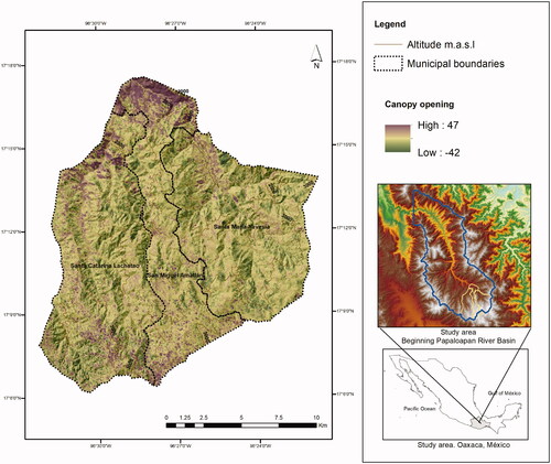
According to the Jenks classification method (see Section 2.6), the spatial representation of the canopy opening was classified into five categories (Figure 5). Wide open areas, or areas with low vegetation cover, are shown in gray tones, while areas with solid vegetation, mainly communities arboreal, are shown in green tones. This result was compared with the information on the land use and vegetation produced by INEGI (2017b), for identifying the behavior of the canopy opening values by type of vegetation. This information serves as a reference for the performance of the resulting opening model and the type of vegetation recognized by INEGI.

Figure 5. Spatial representation of the canopy opening, a result of the map algebra process.

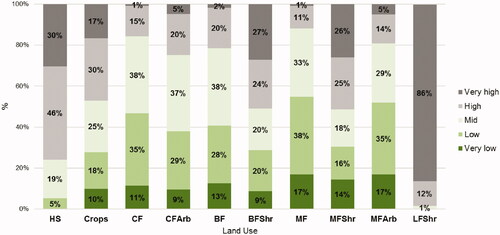
Figure 6 shows the percentage of canopy opening by land use, the data is shown vertically covering 100% of each use, so areas with the greatest openings correspond to human settlement (76%), followed by crops (47%) and low secondary shrub forest (98%). Areas with low and very low openings are represented by the mixed forest (55%), followed by mixed forest with secondary arboreal vegetation (52%), coniferous forest (46%), broadleaf forest (41%), and coniferous forest with secondary arboreal vegetation (30%). The mixed forest with shrubby secondary vegetation occupies 30% of its surface with very low and low opening, while 51% of its surface has high and very high opening ranges. Figure 6 shows the canopy opening degree by vegetation type.

Figure 6. Percentage of canopy opening by vegetation type. AH: Human settlement; Crops: crops; CF: coniferous forest; CFArb: coniferous forest with secondary arboreal vegetation; BF: broadleaf forest; BFShr: broadleaf forest with shrubby secondary vegetation; MF: mixed forest; MFArb: mixed forest with secondary arboreal vegetation; MFShr: mixed forest with secondary shrub vegetation and LFShr: secondary low forest with secondary shrub vegetation.

4. Discussion

The analysis of the canopy opening is important for understanding ecosystems. The spatial distribution of the forest canopy serves to identify their state. A homogeneous canopy coverage has several benefits: there is a greater interception of precipitation, a greater runoff through the trunks, help for recharging aquifers, in addition to climate regulation (Bonan 2008). In contrast, uncovered areas or with little coverage promote landslides or soil erosion due to the lack of protection thereof (Imaizumi et al. 2008).

Using vegetation indices provides a different way of interpreting vegetation cover, in mapping the canopy opening. Vegetation indices make it clear the difference between vegetation and bare soil allowing the assessment of can to be related to the level of conservation of forest areas. However, the intrinsic characteristics of the different types of vegetation must be considered, since some may naturally present a greater opening due to their structure, of species type, the relief condition where they are located, or the date the satellite image was taken. Phenology is also an important factor to be considered. For instance, deciduous vegetation has a different spectral response in the dry season and can potentially be confused or misinterpreted with areas without vegetation cover. MSAVI was the best vegetation index in detecting bare soil, due to the correction factor serves for discriminate it, and consequently, yields better results in the identification of the canopy opening (Gilabert et al. 1997).

Texture filters are a viable option to identify canopy openings. Although these filters are seldom used, they showed good results for the study area. However, it is important to determine the most suitable type of filter, the adequate band, and the window size (Rodríguez 2008). The filter selection criterion was based on the prior recognition of the level of homogeneity (or heterogeneity) of the study area (Anaya et al. 2008).

Factor analysis is a useful tool for identifying significant variables in the study model (Hair et al. 1999) and for reducing redundant information. Here, components 1 and 2 explained 76% of the variation in the data. Brightness is associated to the first component along with vegetation indices with soil adjustment variable. This result is expected since brightness, in a satellite imagery serves to discriminate bare soil. As a support of this result, it must be noticed that, the most significant variables in identifying canopy opening are the MSAVI, SAVI, and DVI, as expected. A positive relationship was found with the slope of the terrain, which influences the opening of the canopy in the vegetation. This relationship can be explained by either, the distribution of species adapted to these conditions or because places with less slope area easily transformed and, therefore, the probability of a land use change increases (Mas et al 2002; Castro 2014).

The resultant spatial representation of the canopy opening showed a good statistical fit. It is evident that the largest openings are in areas with human settlements, crops, and secondary shrubby vegetation. In contrast, areas identified with less openings were coniferous and mixed primary and secondary arboreal forests, due to canopy homogeneity. The broadleaf and mixed forests (pines and oaks) with signs of disturbance and classified as secondary shrubby vegetation by INEGI (2017b), occupy an important percentage of the area with high and very high openings, 51% (each one) broadleaf and mixed forest with secondary vegetation.

This analysis can be used as an indicator of the grade of conservation of the forests. In the study area, it is clearly identified the occupied areas with vegetation and with some stage of deterioration (loss of trees, coverage dominated by shrubs). Therefore, the canopy opening is higher, when compared to better-conserved forests or with a greater abundance of the arboreal component, or even with a more closed canopy, which can be represented with a low or very low opening.

The comparison between opening mapping with specific data (verification), which originally contain the opening percentage information, yield a correlation of r = 0.57. This result can be interpreted as the reliability of the opening map, which can be improved with more hemispheric photographs. This kind of photograph is an inverse and complementary "view" of the sensor. They are taken from bottom to top and provide a good correlation fit with satellite data.

The information derived from the canopy opening map focused on the distribution and spatial structure of temperate forests is very useful for decision-makers, as they can observe where changes in vegetation occur, and if those changes are natural or anthropic. Finally, it must be pointed out that it is an inexpensive and easy-to-replicate methodology, unlike other studies that only use terrestrial instruments to quantify canopy opening.

Acknowledgments

This study is part of the project “Social and environmental susceptibility to extreme events and climate change in the upper Papaloapan basin, Oaxaca”, which was financed by the Support Program for Research and Technological Innovation Projects (PAPIIT-UNAM) [number: IN301118]. To the National Council of Science and Technology (CONACyT), for the financial scholarship granted to carry out doctoral studies in Geography.

Disclosure statement

The authors have no conflict of interest or relevant financial or non-financial interests to disclose.

Additional information

Funding

Program for Research and Technological Innovation Projects (PAP IIT-UNAM), [number: IN301118] and National Council of Science and Technology (CONACyT) for the scholarship.

References

- Alkama R, Cescatti A. 2016. Biophysical climate impacts of recent changes in global forest cover. Science. 351(6273):600–604.
- Anaya J, Londoño RAD, Hernández GMV. 2008. Análisis de textura en imágenes de satélite en el ámbito de la biodiversidad y la estructura en un bosque de los Andes Colombianos. [Texture analysis in satellite images in the field of biodiversity and structure in a forest in the Colombian Andes]. Gestión y Ambiente. 11(3):137–146.
- Baig MHA, Zhang L, Shuai T, Tong Q. 2014. Derivation of a tasseled cap transformation based on Landsat 8 at-satellite reflectance. Remote Sens Lett. 5(5):423–431.
- Bannari A, Morin D, Bonn F, Huete AR. 1995. A review of vegetation indices. Remote Sens Rev. 13(1–2):95–120.
- Bishop J, Pagiola S, Landell-Mills N. 2006. La venta de servicios ambientales forestales. [The sale of forest environmental services]. Secretaría de Medio Ambiente y Recursos Naturales. México: Instituto Nacional de Ecología.
- Bonan GB. 2008. Forests and climate change: forcings, feedbacks, and the climate benefits of forests. Science. 320(5882):1444–1449.
- Buzai GD, Humacata L, Lanzelotti SL, Montes Galbán E, Principi N. 2019. Teoría y métodos de la Geografía Cuantitativa Libro 2: Por una Geografía empírica. [Theory and methods of Quantitative Geography Book 2: For an empirical Geography]. Instituto de Investigaciones Geográficas. Buenos Aires (Argentina): Universidad Nacional de Luján.
- Castro MR. 2014. Modelo espacial de probabilidad a la deforestación en bosques para el estado de Oaxaca.” [Probability spatial model of deforestation in forests for the state of Oaxaca]. Master's thesis. Posgrado en Geografía, UNAM.
- Chica-Olmo M, Abarca-Hernández F. 2000. Computing geostatistical image texture for remotely sensed data classification. Comput Geosci. 26(4):373–383.
- Clark PE, Hardegree SP. 2005. Quantifying vegetation change by point sampling landscape photography time series. Rangeland Ecol Manage. 58(6):588–597.
- Coburn CA, Roberts AC. 2004. A multiscale texture analysis procedure for improved forest stand classification. Int J Remote Sens. 25(20):4287–4308.
- Culbert PD, Pidgeon AM, Louis VS, Bash D, Radeloff VC. 2009. The impact of phenological variation on texture measures of remotely sensed imagery. IEEE J Sel Top Appl Earth Observ Remote Sens. 2(4):299–309.
- Dunkerley D. 2020. A review of the effects of throughfall and stemflow on soil properties and soil erosion. In: Van Stan IIJT, Gutmann E, Friesen J, editors. Precipitation partitioning by vegetation. Cham: Springer, p. 183–214.
- ENVI. 2012. On-line software user’s manual. Boulder (CO): ITT Visual Information Solutions.
- Franklin SE, Hall RJ, Moskal LM, Maudie AJ, Lavigne MB. 2000. Incorporating texture into classification of forest species composition from airborne multispectral images. Int J Remote Sens. 21(1):61–79.
- Frazer GW, Canham CD, Lertzman KP. 1999. Gap Light Analyzer (GLA), Version 2.0: imaging software to extract canopy structure and gap light transmission indices from true-colour fisheye photographs, user’s manual and program documentation. New York: Simon Fraser University, Burnaby, British Columbia, and the Institute of Ecosystem Studies, Millbrook, p. 36.
- Fuller DO. 2006. Tropical forest monitoring and remote sensing: a new era of transparency in forest governance? Singapore J Trop Geo. 27(1):15–29.
- Gilabert MA, González-Piqueras J, García-Haro J. 1997. Acerca de los índices de vegetación. [About vegetation indices]. Revista de Teledetección. 8(1):1–10.
- Hair JF, Anderson RE, Tatham RL, Black WC. 1999. Análisis multivariante. [Multivariate analysis]. Vol. 491. Madrid: Prentice Hall.
- Haralick RM, Shanmugam K, Dinstein IHak. 1973. Textural features for image classification. IEEE Trans Syst, Man, Cybern. SMC-3(6):610–621.
- Harvey D, Rodrigo GL. 1983. Teorías, leyes y modelos en geografía. [Theories, laws and models in geography]. Madrid: Alianza Editorial.
- Huete AR. 1988. A Soil-Adjusted Vegetation Index (SAVI). Remote Sens Environ. 25(3):295–309.
- Hunt ER, Jr, Rock BN. 1989. Detection of changes in leaf water content using near-and middle-infrared reflectances. Remote Sens Environ. 30(1):43–54.
- Imaizumi F, Sidle RC, Kamei R. 2008. Effects of forest harvesting on the occurrence of landslides and debris flows in steep terrain of central Japan. Earth Surf Process Landforms. 33(6):827–840.
- Instituto Nacional de Estadística y Geografía (INEGI). 2005. Cuaderno estadístico del estado de Oaxaca. [Statistical notebook of the state of Oaxaca]. México: INEGI.
- Instituto Nacional de Estadística y Geografía (INEGI). 2010. Censo de Población y Vivienda. [Census of population and housing]. México: INEGI.
- Instituto Nacional de Estadística y Geografía (INEGI). 2017a. Continuo de Elevaciones Mexicano versión 3.0 (CEM). [Continuous Mexican elevations]. México: INEGI.
- Instituto Nacional de Estadística y Geografía (INEGI). 2017b. Conjunto de datos vectoriales de uso de suelo y vegetación escala 1:250,000, Serie VI (Capa unión). [Vegetation and land use vector data set]. México: INEGI.
- INTERGRAPH. 2012. Erdas versión 13.0. https://download.hexagongeospatial.com/en/search
- Jenks GF. 1967. The data model concept in statistical mapping. Int Yearbk Cartogr. 7:186–190.
- Jones HG, Vaughan RA. 2010. Remote sensing of vegetation: principles, techniques, and applications. Oxford: Oxford University Press.
- Kauth RJ, Thomas GS. 1976. The tasseled cap–a graphic description of the spectral-temporal development of agricultural crops as seen by Landsat. LARS Symposia, 159.
- Lee SM, Abbott AL, Clark NA, Araman PA. 2005. Active contours on statistical manifolds and texture segmentation. Image Processing, 2005. ICIP 2005. IEEE International Conference on, Vol. 3, p. III–828. IEEE. DOI: https://doi.org/10.1109/ICIP.2005.1530520.
- Mas JF, Velázquez A, Castro R, Schmitt A. 2002. Una evaluación de los efectos del aislamiento, la topografía, los suelos y el estatus de protección sobre las tasas de deforestación en México. [An assessment of the effects of isolation, topography, soils, and protected status on deforestation rates in Mexico]. R. Raega - O Espaço Geográfico em Análise (RAEGA). 6:61–73.
- Meléndez Pastor I, Navarro Pedraño J, Gómez I, Koch M. 2009. Análisis de series temporales de vegetación obtenidas mediante teledetección como herramienta para el seguimiento de procesos de desertificación. [Analysis of vegetation time series obtained by remote sensing as a tool for monitoring desertification processes]. Congreso Internacional Sobre Desertificación en Memoria Del Profesor John B. Thornes, 339–342.
- Muñoz CAC. 2013. Use of satellite images to assess the effects of land cover change on direct runoff from an Andean basin [doctoral dissertation]. Universidad de Concepción. Chile.
- Norman M. 1984. The primary source: tropical forests and our future. Vol. xxxii. New York: W. W. Norton, p. 416, p: ill., maps.
- Pardo A, Ruiz MÁ. 2002. SPSS 11: guide for data analysis. New York: McGrawHill.
- PAWS Statistics 21 (Release 21.0.0). 2010. Nikiski (AK): Polar Engineering and Consulting.
- Percy KE. 1989. Vegetation, soils, and ion transfer through the forest canopy in two Nova Scotia lake basins. Water Air Soil Pollut. 46(1–4):73–86.
- Potapov P, Turubanova S, Hansen MC. 2011. Regional-scale boreal forest cover and change mapping using Landsat data composites for European Russia. Remote Sens Environ. 115(2):548–561.
- Poyatos R, Latron J, Llorens P. 2003. Land use and land cover change after agricultural abandonment. Mt Res Dev. 23(4):362–369.2.0.CO;2]
- Qi J, Chehbouni A, Huete AR, Kerr YH, Sorooshian S. 1994. A modified soil adjusted vegetation index. Remote Sens Environ. 48(2):119–126.
- Qi J, Huete AR, Moran MS, Chehbouni A, Jackson RD. 1993. Interpretation of vegetation indices derived from multi-temporal SPOT images. Remote Sens Environ. 44(1):89–101.
- Rahman S, Mesev V. 2019. Change vector analysis, tasseled cap, and NDVI-NDMI for measuring land use/cover changes caused by a sudden short-term severe drought: 2011 Texas event. Remote Sens. 11(19):2217.
- Rodríguez JG. 2008. Estado Actual de la Representación y Análisis de Textura en Imágenes. Reporte Técnico. [Current State of the Representation and Analysis of Texture in Images. Technical report]. Reconocimiento de patrones. Habana (Cuba): Centro de Aplicaciones de Tecnología Avanzada (CENATAV).
- Rouse J, Jr, Haas RH, Schell JA, Deering DW. 1974. Monitoring vegetation systems in the Great Plains with ERTS. Remote sensing. College Station (TX): Texas A&M University.
- Schanda E. 2012. Physical fundamentals of remote sensing. Cham: Springer Science & Business Media.
- Schroeder TA, Cohen WB, Song C, Canty MJ, Yang Z. 2006. Radiometric correction of multi-temporal Landsat data for characterization of early successional forest patterns in western Oregon. Remote Sens Environ. 103(1):16–26.
- Shvidenko A, Barber CV, Persson R, González P, Hassan R. 2005. Forest and woodland systems. In: R. Hassan, R. Scholes, & N. Ash, editors. Ecosystems and human well-being: current state and trends, Vol. 1, findings of the condition and trends working group of the millennium ecosystem assessment. Washington (DC): Island Press, p. 587–614.
- Tucker CJ. 1979. Red and photographic infrared linear combinations for monitoring vegetation. Remote Sens Environ. 8(2):127–150.
- U.S. Geological Survey (USGS). 2019. Landsat 8 (L8) data users handbook. Version 5.0. Reston (VA): USGS.
- Welles JM, Cohen S. 1996. Canopy structure measurement by gap fraction analysis using commercial instrumentation. J Exp Bot. 47(9):1335–1342.
- Wulder M. 1998. Optical remote-sensing techniques for the assessment of forest inventory and biophysical parameters. Prog Phys Geogr. 22(4):449–476.
- Zhu X, Liu D. 2014. Accurate mapping of forest types using dense seasonal Landsat time-series. ISPRS J Photogramm Remote Sens. 96:1–11.