Comparative study of forest biomass and carbon stocks of Margalla Hills National Park, Pakistan

Abstract

Forests can play an important role in climate change mitigation. However, limited information is available worldwide regarding forest carbon and biomass stocks. Financial mechanisms such as ‘reducing emissions from deforestation and forest degradation and the role of conservation of forest carbon, sustainable management of forests and enhancement of forest carbon stocks’ (REDD+) also emphasize the quantification of forest biomass and carbon. This study aimed to estimate the forest biomass in two forests of Margalla Hills National Park (MHNP): Sub-tropical Chir Pine Forest (SCPF) and Sub-tropical Broadleaved Evergreen Forest (SBEF). For this, circular sampling plots of a 20 m radius were used for the collection of the variables, “diameter at breast height (DBH) and height”. Statistical analysis was done for exploring regression relationships between the variables. We found a mean Aboveground Carbon (AGC) of 73.36 ± 32.55 Mg C ha⁻¹ in SCPF and a mean AGC of 16.88 ± 25.81 Mg C ha⁻¹ in SBEF. The mean Aboveground Biomass (AGB) for SCPF was recorded as 146.73 ± 65.11 Mg ha⁻¹, while for SBEF it was 33.77 ± 51.63 Mg ha⁻¹. It was therefore concluded that the SCPF had higher mean AGB and mean AGC than the SBEF. Similar differences were also noticed in the structural characteristics of the two forests. These could be valuable information while designing sustainable management plans and afforestation programmes for the future and also for accessing nature-based funding such as REDD+.

Keywords:

• Forests
• aboveground biomass
• carbon
• REDD
• +
• sustainable management

Introduction

Climate change is one of the greatest threats of recent times (Poškus and Žukauskienė 2017; Soutter and Mõttus 2020). It is defined as the shift in climate patterns, which is mainly caused by greenhouse gas (GHG) emissions (Fawzy et al. 2020). CO₂ has mainly received widespread attention, among other GHG emissions, due to its increasing levels which have resulted in higher temperatures, shifting precipitation patterns, unpredictable extreme events, etc. (Reichstein et al. 2013). Globally, the CO₂ concentration has risen from approximately 277 parts per million (ppm) in 1750, which was the beginning of the Industrial Era, to 409.85 ± 0.1 ppm in 2019 (Joos and Spahni 2008; Dlugokencky and Tans 2020). Anthropogenic activities have been the main culprit causing climate change (Xi-Liu and Qing-Xian 2018). Deforestation and forest degradation, for instance, have led to an increase in GHG emissions from 490 ± 180 Gt CO₂ in 1970 to 680 ± 300 Gt CO₂ in 2010 (IPCC 2007). The severity of climate change can also be seen from the fact that the global surface temperature was 1.09 °C higher in 2011–2020 than in 1850–1900 (IPCC 2023).

Aboveground Biomass (AGB), an important global measurement standard for climate change mitigation activities, generally, accounts for 70% to 90% of total forest biomass (FAO 2010). AGB is “all the biomass of living vegetation, both woody and herbaceous, above the soil including stems, stumps, branches, bark, seeds, and foliage” (FAO 2020a). It is usually measured in metric tonnes of dry matter per hectare (e.g. t ha⁻¹ or Mg ha⁻¹) or in metric tonnes of carbon per hectare (e.g. t C ha⁻¹ or Mg C ha⁻¹) (Omar et al. 2017; Rodríguez-Veiga et al. 2017). It can only be measured directly and accurately through destructive sampling, where the trees are cut down and dry weights are calculated using oven-drying methods, which are regressed against the volumes estimated using volumetric methods (Wilkes et al. 2018). However, this is labor intensive, expensive, often impractical, and rarely adopted (Dumitrașcu et al. 2020). Destructive sampling is also not recommended for places where there is threatened flora and fauna (Kumar and Mutanga 2017). Nondestructive methods include the use of already available allometric equations for the estimation of AGB without cutting down the trees (Rodríguez-Veiga et al. 2017; Debastiani et al. 2019). The allometric equations are statistical models based on the forest inventory data such as diameter at breast height (DBH), height, wood density, and forest type (Chave et al. 2004). The forest inventory data is one of the most reliable sources for carbon estimation globally (Zhao et al. 2019). The choice of the allometric equation is, however, critical, where an inconsiderate selection of the equation may lead to errors of up to 79% (Clark et al. 2001). For reduction in uncertainties in AGB estimation, site and species-specific allometric equations have been emphasized (Soares and Schaeffer-Novelli 2005).

The other nondestructive method, involving forest inventory data, includes the use of the Biomass Expansion Factors (BEF) and Wood Density (WD), which are used to convert the tree volume to the AGB (Asrat et al. 2020; Hossain et al. 2020). BEF is unitless and is defined as “the ratio of oven-dried tree biomass to either the commercial or stem oven-dried biomass including bark” (Schepaschenko et al. 2018). BEF approach is not flexible in terms of the use of various variables such as the allometric equations. In the BEF approach, only the tree volume, BEF, and wood density are used for the estimation of AGB, as mentioned before. Other forest carbon pools include; Belowground Biomass (BGB), deadwood, litter, and soil carbon (Buchholz et al. 2014). BGB is “all the biomass of live roots. Fine roots of less than 2 mm diameter are excluded because these often cannot be distinguished empirically from soil organic matter or litter” (FAO 2020a). Deadwood is “all the non-living woody biomass not contained in the litter, either standing, lying on the ground, or in the soil. It includes wood lying on the surface, dead roots, and stumps larger than or equal to 10 cm in diameter or any other diameter used by the country” (FAO 2020a). Litter includes “all non-living biomass with a diameter less than the minimum diameter for dead wood (e.g. 10 cm), lying dead in various states of decomposition above the mineral or organic soil” (FAO 2020a). Soil carbon is the "organic carbon in mineral and organic soils (including peat) to a specified depth chosen by the country and applied consistently through the time series” (FAO 2020a).

Generally, forest biomass is an indicator of its carbon status since carbon forms half of the dry weight of a tree (Vicharnakorn et al. 2014; Raihan et al. 2021). Agriculture, Forestry and Other Land Use (AFOLU) offers one of the largest potentials for GHG emissions reduction through reduced deforestation and forest degradation, amounting to 0.4–5.8 Gt CO₂-eq year⁻¹ (IPCC 2019). However, according to the fourth assessment report of the Intergovernmental Panel on Climate Change (IPCC) (IPCC 2007), there is a limited amount of information available regarding forest biomass and carbon status at both national and regional levels. For tackling climate change, large-scale implementation of mitigation responses would be required (IPCC 2023). The United Nations Framework Convention on Climate Change (UNFCCC) has also recognized the AGB as an Essential Climate Variable (ECV) (Omar et al. 2017). ECVs are the physical, biological, and chemical variables or groups of variables that critically affect the Earth’s climate (Bojinski et al. 2014). The ‘reducing emissions from deforestation and forest degradation and the role of conservation of forest carbon, sustainable management of forests and enhancement of forest carbon stocks’ (REDD+) is also a result-based financial incentive for developing countries to counteract deforestation (Maraseni et al. 2014; Köhl, Neupane, et al. 2020) since 98% of the deforestation is occurring in developing countries (FAO 2020b). REDD + is also one of the cheapest climate mitigation options for tackling climate change (Golub et al. 2018; Raihan et al. 2019; Raihan and Said 2022). However, such global initiatives require quantification of forest biomass and carbon (Campbell 2009; Koch 2010).

Pakistan’s forest covers 4.6% of its total land area, according to the FAO (2020). It is a low forest cover country (LFCC) (Aftab and Hickey 2010). Forest per capita in Pakistan is only 0.03 ha compared to the global average of 1 ha (Ali et al. 2020a). Despite low forestry resources, Pakistan faced one of the highest deforestation rates in the world losing 0.94% annually between 2010 to 2020 (FAO 2020b). One of the main pressures on forestry resources in Pakistan has been the high reliance of local communities on these resources often for their subsistence (Shahbaz et al. 2007; Hussain, Zhou, et al. 2019). Such types of pressures are further aggravated by the increasingly adverse effects of climate change (Khan et al. 2020). Like many developing countries, Pakistan has contributed only a meager amount of 0.8% to the world’s GHG emissions (Hussain, Butt, et al. 2019; Sajid 2020).

Forest biomass quantification becomes essential for the areas, such as the study area for this research, Margalla Hills National Park (MHNP), which are prone to increasing local pressures. The case of MHNP even becomes more unique, since it is adjoined with the capital city of Pakistan. The location is, thus, exposing the MHNP to encroachment due to the increasing population of the city. This, along with other internal pressures i.e. local communities’ increasing dependencies on forest resources, forest fires due to humans, limestone extraction, etc. within the MHNP, are threatening the unique ecological resources of the MHNP. Forest biomass assessments can therefore help in the identification of the carbon potential of the MHNP which can be used for accessing financial resources such as REDD+. The adequate financial resources, in turn, can help to develop and implement suitable sustainable management strategies, that can involve local communities of the MHNP in participatory management, since they depend on forestry resources. Given the aforementioned, the study aimed at the quantification of forest biomass at the MHNP. Specific objectives included i) Assessment of the AGB and Aboveground Carbon (AGC) of the trees of two forest types of the MHNP: Sub-tropical Chir Pine Forest (SCPF) and Sub-tropical Broadleaved Evergreen Forest (SBEF) ii) Determination of the structural characteristics (i.e. volume, basal area, DBH, and height) of the two forests iii) Identification of the contribution of individual tree species to each forest type iv) Comparison of the AGC between the two forests v) Regression analysis of the main tree species of the two forest types involving following variables: AGB, volume, basal area, DBH, and height. Since there is a lack of allometric equations in Pakistan for local tree species for AGB estimation, the BEF approach was used for the AGB assessment (Ismail et al. 2018).

Materials and methods

Study area

The MHNP has an area of 17,386 ha (Figure 1) (Mannan et al. 2018), which is spread between 73°7’3.32” E, 33°41’59.61” N, and 73°1’34.07” E, 33°45’2.87” N (WWF-Pakistan 2009). It has an elevation of 410.56 m to 1190.85 m. MHNP has a rough topography and some steep slopes and gullies. MHNP was declared a National Park on 27^th April 1980 under Section 21(1) of the Islamabad Wildlife (Protection, Conservation, and Management) Ordinance, 1979 (Himalayan Wildlife Foundation 2007). Before 1960, much of the area was classified as a ‘Reserve Forest’. Later, however, the area was declared a ‘Wildlife Sanctuary’ under the West Pakistan Wildlife Protection Ordinance, 1959 (Himalayan Wildlife Foundation 2007). It has 27 villages located within its boundaries. The climate is semi-arid. The area lies in the monsoon belt, and it experiences two rainy seasons: Winter rains from January to March, and summer rains from July to September. During the winter season, the temperature ranges from 1–15 °C, and during the summer season, the temperature ranges from 20–40 °C. It has five seasons: winter (December-February), spring (March-April), summer (May-June), monsoon (July-September), and autumn (November) (Anwar and Chapman 2000). The average annual rainfall is 1,000 mm (Himalayan Wildlife Foundation 2007). The soil is mainly composed of limestone (Butt et al. 2015). The flora of the MHNP includes 101 families, 548 genera, and 608 species (Akbar 2012).

Figure 1. (a) Location of Study Area in Pakistan (b) Study Area with Land Cover Classes and Location of Sampling Plots in SCPF and SBEF.

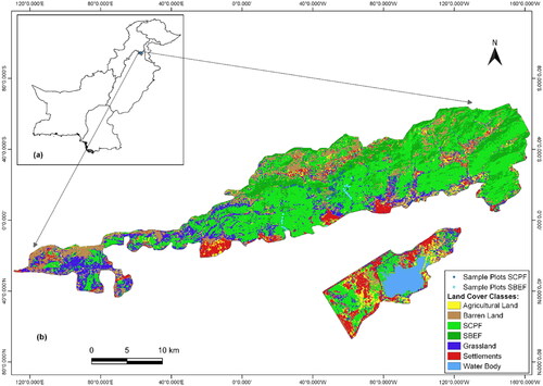
The MHNP is composed of two types of forests, SCPF and SBEF (Mannan et al. 2018). The SCPF is predominantly located above 900 m (Himalayan Wildlife Foundation 2007) and is mainly characterized by the Pinus roxbughii Sarg. that forms the main canopy. Other areas in Pakistan where this forest is found include Murre Hills, Swat, Shinkiari, etc. (Nizami 2010). The SBEF is classified as an arid forest which is usually composed of branchy trees and varies from a complete closure, owing to favorable conditions, to scattered trees/shrubs on the drier sites (Sheikh 1993). These are low forests with species that are mostly thorny and often with evergreen leaves (Sheikh 1993). The larger trees can be seen in valleys where deep soil and adequate water are available. Generally, these forests are encountered by noticeable erosion and are characterized by gullies and deep ravines, which makes the rocks and boulders common features. In other areas in Pakistan, these forests are generally found in Kala Chitta Mountains (Kherimurat), salt ranges, Malakand Agency, Parachinar, Loralai, Sohawa, etc. (Nizami 2010).

Field inventory measurements

There were 46 sampling plots in the SCPF, and 31 in the SBEF, using a stratified random sampling approach. The sampling plots were circular with a radius of 20 m and an area of 0.126 ha (Pearson et al. 2005). The DBHs of all the trees above 5 cm, in the sampling plots, were measured with the help of the DBH tape above the ground level at 1.3 m (Laar and Akça 2007). The Vertex IV (Haglöf Sweden, AB), along with its transponder, was used for the estimation of tree heights in the sampling plots. The Vertex IV has a mean error of −0.66 m. Overall, there were 640 trees measured from the SCPF and 443 trees measured from the SBEF. The coordinates were also recorded from the center of the plots using handheld Global Positioning System (GPS) device (Garmin GPS 60 Marine). The GPS device can have an error of 3–4 m.

Data analysis

Structural and AGB analysis

The quadratic mean diameter (cm) for each plot was computed as follows (Eq. 1(1) $$\mathbf{Mean} \mathbf{DBH} =\mathrm{ }\sqrt{\frac{{{\mathit{DBH}}_i}^2}{n}}$$(1) ) (Iles and Wilson 1977); (1) $$\mathbf{Mean} \mathbf{DBH} =\mathrm{ }\sqrt{\frac{{{\mathit{DBH}}_i}^2}{n}}$$(1)

Where n is the total number of trees. The quadratic mean diameter in this research was referred to as the mean DBH. The tree volume (m³) was recorded using the following formula (Eq. 2(2) $$\mathbf{Tree} \mathbf{Volume} =\mathrm{ }(\mathrm{\pi }/4)\mathrm{ }\times \mathrm{ }{\mathrm{DBH}}^2\mathrm{ }\times \text{ H }\times \mathrm{ }\mathrm{FF}$$(2) ) (Philip 1994); (2) $$\mathbf{Tree} \mathbf{Volume} =\mathrm{ }(\mathrm{\pi }/4)\mathrm{ }\times \mathrm{ }{\mathrm{DBH}}^2\mathrm{ }\times \text{ H }\times \mathrm{ }\mathrm{FF}$$(2)

Where H (m) is the height of a tree and FF (unitless) is the form factor. The form factor of a tree is defined as “the stem volume which is expressed as the proportion of the cylinder volume of the same height which has a diameter equal to the stem diameter at the selected reference point” (Laar and Akça 2007). For this research, a form factor of 0.45 was used for Pinus roxburghii, and for other broadleaved species, a form factor of 0.59 was used as suggested by (Gray 1956).

The stand basal area is defined as the sum of the cross-sectional area of the stems at breast height and expressed per unit of ground area (West 2009). The basal area (m²) was calculated by using the following formula (Eq. 3(3) $$\mathbf{Basal} \mathbf{Area} = \frac{{\left(\mathrm{DBH}\right)}^2\times \pi }{4}$$(3) ) (Köhl et al. 2006); (3) $$\mathbf{Basal} \mathbf{Area} = \frac{{\left(\mathrm{DBH}\right)}^2\times \pi }{4}$$(3)

The density is the number of trees per unit area (West 2009). Initially, the AGB (Kg) was calculated as follows (Eq. 4(4) $$\mathbf{AGB} =\text{ Volume }\times \text{ Wood Density }\times \mathrm{ }\mathrm{BEF}$$(4) ) (Brown et al. 1999; Pandey et al. 2019); (4) $$\mathbf{AGB} =\text{ Volume }\times \text{ Wood Density }\times \mathrm{ }\mathrm{BEF}$$(4)

The ‘Wood Density (Kg m³)’ is defined as “the amount of actual wood substance which is present in a unit volume of wood” (Zobel and Jett 1995). Wood densities for sampled tree species were sourced from literature (see Supplementary Table 1). The BEF of 1.51 was used for Pinus roxburghii and 1.59 was used for all other broadleaved tree species which were encountered during the sampling process (Haripriya 2000). The ‘AGB (Kg)’ was converted to ‘AGB Mg (megagram)’ by dividing the former by 1000. The ‘AGB’ was converted to ‘Aboveground Carbon (AGC)’ by using the carbon conversion factor of 0.5 (Köhl, Ehrhart, et al. 2020). The above-mentioned variables: Volume (m³), Basal Area (m²), Density, AGB (Mg), and AGC (Mg C) were scaled up to ha by dividing the variables by 0.1 (Torres et al. 2020).

Statistical analysis

Means and standard deviations were calculated for the variables (mean ± SD). The data was checked for the normality distribution, for which Shapiro-Wilk test was used. Since the data were not normally distributed, the Wilcoxon rank sum test was used for probing the statistical difference between the variables. The significance levels of 0.01, 0.05, and 0.1 were used for investigating the differences between the variables of the two forest types. The Spearman correlation coefficient, which is a non-parametric measure, was used for the correlation analysis of the variables since the data was not normally distributed (Best and Roberts 1975). For the Spearman correlation coefficient, which ranges between −1 to 1, the interpretation was done following Ratner (2009), for assisting in understanding the relationships based on different levels; 1) 0 indicating no relationship 2) +1 indicating perfect positive linear relationship 3) −1 indicating perfect negative relationship 4) values between (0 and 0.3) indicating weak positive linear relationship and values between (-0.3 and 0) weak negative relationship 5) values between (0.3 and 0.7) indicating moderate positive linear relationship and values between (-0.3 and −0.7) indicates a moderate negative linear relationship 6) values between (0.7 and 1) indicating a strong positive linear relationship and values between (-0.7 and −1) indicating strong negative linear relationship. The Spearman correlation coefficient, Shapiro-Wilk test and Wilcoxon rank sum test were determined using the ggpubr package (Kassambara 2023) in the RStudio (R Core Team 2023). Regression analysis was also performed in RStudio, using the stats package in R (R Core Team 2023). Regression analysis was done for analyzing the relationship between every two variables of interest for the three dominant species (highest number of measured species) for the two forest types i.e. i) Pinus roxburghii Sarg. for SCPF ii) Bauhinia variegata L. and Grewia optiva J. R. Drumm. ex Burret for SBEF. Linear regression analysis was performed for linear relationship and a power curve was used in case of a non-linear relationship between the variables i.e. DBH and height; volume and basal area; DBH and AGB. Significance levels of 0.01, 0.05, and 0.1 were used to explore the statistical significance, and the Coefficient of Determination (R²) was then used for assessing the strength of the statistical relationship between the two variables. The evaluation of the strengths of the R² was based on the following; 1) 0.19 (weak) 2) 0.33 (moderate) and 3) 0.67 (substantial/significant) (Chin 1998). The negative sign implies the negative statistical relationship between the variables.

Results

Structural characteristics of the two forests of the MHNP

The mean AGC for SCPF was higher than the SBEF. The mean AGC for SCPF was 73.36 ± 32.55 Mg C ha⁻¹ and the mean AGC for SBEF was 16.88 ± 25.81 Mg C ha⁻¹ (Table 1). The mean AGB of the SCPF was also higher than the mean AGB of the SBEF. The mean AGB for SCPF was 146.73 ± 65.11 Mg ha⁻¹ and the mean AGB for SBEF was 33.77 ± 51.63 Mg ha⁻¹. High significant differences were recorded between the AGB and AGC of the two forests (W = 43, p < 0.01). SCPF was also greater than SBEF for all the other structural variables, except for the mean density ha⁻¹ (Table 1).

Table 1. Structural characteristics of forests of MHNP.

Forests	SCPF	SBEF	Combined
Mean AGC (Mg C ha^−1)	73.36 ± 32.55^a	16.88 ± 25.81^b***	50.62 ± 40.84
Mean AGB (Mg ha^−1)	146.73 ± 65.11^a	33.77 ± 51.63^b***	101.25 ± 81.68
Mean Tree Volume (m^3 ha^−1)	198.75 ± 87.76^a	37.82 ± 50.38^b***	133.96 ± 108.96
Mean Basal Area (m^2 ha^−1)	14.48 ± 4.80^a	4.28 ± 3.43^b***	10.37 ± 6.60
Mean Density ha^−1	139.13 ± 22.88^a	142.90 ± 32.37^a	140.64 ± 26.96
Mean DBH (cm)	36.37 ± 6.51^a	18.64 ± 6.03^b***	29.23 ± 10.77
Mean Tree Height (m)	27.34 ± 3.67^a	10.62 ± 1.99^b***	20.61 ± 8.81

Mean ± SD.

Different letters indicate on the superscripts denote the significant differences (Wilcoxon Rank Sum Test; ***p < 0.01, **p < 0.05, *p < 0.1) between the two forests.

Correlation analysis of structural variables of two forests with the AGB

Spearman correlation coefficients were calculated between the AGB and other structural characteristics of the SCPF (Table 2). Strong positive and significant correlations were recorded between AGB and volume, basal area, mean DBH, and mean tree height.

Table 2. Spearman correlation coefficients for SCPF (n = 46).

Variables	Volume (m^3 ha^−1)	Basal Area (m^2 ha^−1)	Mean DBH (cm)	Mean Tree Height (m)
AGB (Mg ha^−1)	0.99^a	0.94^a	0.91^a	0.75^a
Volume (m^3 ha^−1)	1	0.94^a	0.91^a	0.75^a
Basal Area (m^2 ha^−1)		1	0.87^a	0.59^a
Mean DBH (cm)			1	0.71^a

^aCorrelation is significant at the 0.05 level.

Spearman correlation coefficients were also calculated between AGB and other structural characteristics of the SBEF (Table 3). Strong positive and significant correlations were recorded between AGB and volume, basal area, mean DBH, and mean tree height.

Table 3. Spearman correlation coefficients for the SBEF (n = 31).

Variables	Volume (m^3 ha^−1)	Basal Area (m^2 ha^−1)	Mean DBH (cm)	Mean Tree Height (m)
AGB (Mg ha^−1)	0.95^a	0.89^a	0.87^a	0.68^a
Volume (m^3 ha^−1)	1	0.93^a	0.90^a	0.70^a
Basal Area (m^2 ha^−1)		1	0.89^a	0.52^a
Mean DBH (cm)			1	0.64^a

^aCorrelation is significant at the 0.05 level.

DBH distribution of the two forests of MHNP

The DBH interval with the highest number of stems was recorded as 35–40 cm for the SCPF (Figure 2). It was followed by the DBH interval of 25–30 cm and the DBH interval of 20–25 cm. The total number of 114 stems was recorded in the DBH interval class 35–40 cm, which formed 17.81% of the total stems of the SCPF. Overall, there were 640 stems recorded for the SCPF. The DBH interval 25–30 cm recorded 107 stems, which formed 16.72% of the total stems, for the DBH interval 20–25 cm, 85 stems were recorded, forming 13.28% of the total stems of the SCPF. The maximum DBH was recorded as 67 cm, for Pinus roxburghii, and the minimum DBH as 10 cm, also for Pinus roxburghii, for the SCPF.

Figure 2. DBH Distribution of the Two Forests of the MHNP.

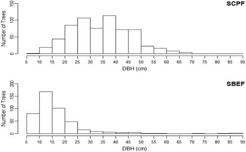
For SBEF, the DBH interval of 10–15 cm contained the highest number of stems (Figure 2). It included 167 stems, which formed 37.70% of the total stems of the SBEF. There were overall 443 stems recorded for the SBEF. The DBH interval 15–20 cm recorded the second highest number of trees with 102 trees, constituting 23.02% of the total number of trees. The DBH interval of 5–10 cm formed the interval with the third highest number of trees of 80, constituting 18.06% of the total stems. The highest DBH was recorded as 87 cm for Ficus palmata subsp. virgata and the lowest DBH was recorded as 5.5 cm for Grewia optiva for the SBEF.

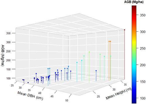
AGB (Mg ha⁻¹) against mean DBH (cm) and mean tree height (m)

The AGB (Mg ha⁻¹) of the SCPF increases with the increasing mean DBH (cm) and mean tree height as shown in the 3D graph (Figure 3).

Figure 3. AGB (Mg ha⁻¹) of SCPF against the Mean DBH (cm) and the Mean Height (m).

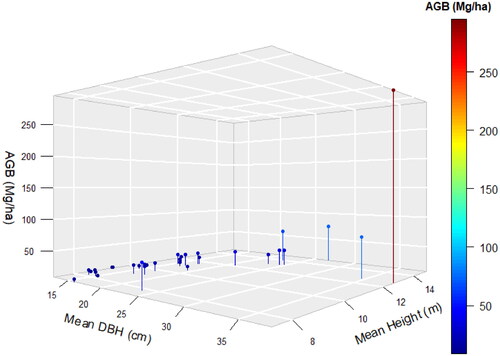
The AGB (Mg ha⁻¹) of the SBEF has shown an erratic pattern against the mean DBH (cm) and the mean tree height (m) as can be seen in the 3D graph (Figure 4).

Figure 4. AGB (Mg ha⁻¹) of SBEF against the Mean DBH (cm) and the Mean Height (m).

AGC of the different trees species in the two forests of the MHNP

Pinus roxburghii contributed the highest percentage of 98.85%, which constitutes 3336.13 Mg C ha⁻¹, of the overall total AGC of 3374.80 Mg C ha⁻¹ of the SCPF (Table 4). The Bombax cieba formed 0.81%, with 27.01 Mg C ha⁻¹, and the Bauhinia variegata contributed 0.34%, with 11.64 Mg C ha⁻¹, to the total AGC of the SCPF of MHNP.

Table 4. AGC contribution of different trees species in SCPF.

Species	Total AGC (Mg C ha^−1)	AGC Percentage (%)
Pinus roxburghii Sarg.	3336.13	98.85
Bombax ceiba L.	27.01	0.81
Bauhinia variegata L.	11.66	0.34
Total	3374.80	100

For the SBEF, Eucalyptus camaldulensis formed the highest contribution of 33.65%, with 176.14 Mg C ha⁻¹, in the total AGC (Table 5). Ficus palmata subsp. virgata and Bauhinia variegata formed the second and third highest contributions with 94.24 Mg C ha⁻¹, 18%, and 73.35 Mg C ha⁻¹, 14.01%, respectively, in the total AGC of the SBEF of the MHNP. Similarly, Acacia modesta, Bombax ceiba, and Grewia optiva followed with 42.29 Mg C ha⁻¹ (8.08%), 36.94 Mg C ha⁻¹ (7.06%), and 30.84 Mg C ha⁻¹ (5.89%). The lowest contributions were recorded for Ficus benghalensis with 0.7%, constituting 3.67 Mg C ha⁻¹, and Flacourtia indica, with 0.1%, forming 0.51 Mg C ha⁻¹, of the total AGC of the SBEF of the MHNP.

Table 5. AGC contribution of different trees species in SBEF.

Species	Total AGC (Mg C ha^−1)	AGC Percentage (%)
Eucalyptus camaldulensis Dehnh.	176.14	33.65
Ficus palmata subsp. virgata Forssk.	94.24	18
Bauhinia variegata L.	73.35	14.01
Acacia modesta Wall.	42.29	8.08
Bombax ceiba L.	36.94	7.06
Grewia optiva J. R. Drumm. ex Burret	30.84	5.89
Mallotus philippensis (Lam.) Muell. Arg.	20.78	3.97
Cassia fistula L.	10.99	2.1
Broussonetia papyrifera (L.) L'Herit ex Vent.	9.86	1.88
Celtis australis L.	9.29	1.77
Albizia lebbeck (L.) Benth	8.44	1.61
Ziziphus mauritiana Lam.	6.14	1.17
Ficus benghalensis L.	3.67	0.7
Flacourtia indica (Burm. f.) Merr.	0.51	0.1
Total	523.47	100

Regression analysis of the main tree species of the two forests

All the equations were highly significant (Table 6). The R² values for all the equations ranged between 0.36 to 0.98. The Bauhinia variegata recorded a moderate statistical association between the DBH and height (R² = 0.36). The highest R² value (0.98) was recorded for the Pinus roxburghii, for its power curve regression, between the DBH and AGB.

Table 6. Relationship type, equation, and R² value of main trees species from MHNP.

Species	Parameters	Relationship Type	Equation	R^2
Pinus roxburghii	DBH & H	Linear	H = 11.55 + 0.45DBH	0.74***
	BA & V	Linear	V=-58.96 + 17.87BA	0.96***
	DBH & AGB	Power Curve	AGB = 0.0007 * DBH^2.62	0.98***
Bauhinia variegata	DBH & H	Linear	H = 5.60 + 0.25DBH	0.36***
	BA & V	Linear	V = 0.07 + 5.86BA	0.92***
	DBH & AGB	Power Curve	AGB = 0.002 * DBH^2.21	0.93***
Grewia optiva	DBH & H	Linear	H = 4.69 + 0.33DBH	0.42***
	BA & V	Linear	V=-0.20 + 5.95BA	0.97***
	DBH & AGB	Power Curve	AGB = 0.002 * DBH^2.33	0.59***

H: height (m); V: volume (m³ ha⁻¹); BA: basal area (m² ha⁻¹); AGB (Mg ha⁻¹); DBH (cm).

*** p < 0.01, ** p < 0.05, * p < 0.1.

Discussion

AGB and AGC of the SCPF

Table 7 shows the AGC estimations of the SCPF from different studies in Pakistan and the Azad Jammu and Kashmir (AJK) region. The mean AGC estimated through this study, 73.36 Mg C ha⁻¹, is higher than the mean AGC recorded by Amir et al. (2018) for SCPF which was 40 Mg C ha⁻¹ at the Murree Hills, Pakistan, and by Ali et al. (2020b) who reported 24.77 Mg C ha⁻¹ for the SCPF of the Khyber Pakhtunkhwa (KPK) Province, Pakistan. The other studies in Pakistan by Nizami (2012) and Mannan et al. (2019) have recorded higher mean AGC estimates compared to this study. The other estimate provided by Amir et al. (2018), 264.5 Mg C ha⁻¹, for the SCPF at Murree Hills, Pakistan, is also higher than this study. The study by Shaheen et al. (2016) for Muzaffarabad District, AJK, also recorded higher AGC for SCPF compared to this study. In three of these studies by Amir et al. (2018), Nizami (2012), and Mannan et al. (2019), the belowground carbon (BGC) was also included in the mean AGC. The BGC generally constitutes 20% of the AGC (Cairns et al. 1997). The result of this study is also in agreement with the estimates provided by Singh et al. (1985) who reported AGC of 35 to 75.2 Mg C ha⁻¹ for the degraded forests of the Central Himalayan, India. The lower AGC for the SCPF can be attributed to the lower AGB yield of the study area (Segura and Kanninen 2005). This low yield may also be due to anthropogenic activities and the natural disturbances occurring in the area (Bhadwal and Singh 2002; Rossi et al. 2007). The depletion in the AGC of the forest ecosystems is mainly attributed to forest degradation in developing countries (Pant and Tewari 2014).

Table 7. Mean AGC of SCPF Reported by Different Studies.

Authors/Workers	Region/Study Area	Mean AGC (Mg C ha^−1)
(Amir et al. 2018)	Murre Hills, Pakistan	40 to 264.5
(Nizami 2012)	Ghoragali and Lehterar, Pakistan	119 and 92
(Shaheen et al. 2016)	Muzaffarabad District, AJK	154 and 264.5
(Mannan et al. 2019)	Foothills of the Himalayan mountains, Pakistan	173.38
(Ali et al. 2020a)	KPK, Pakistan	24.77
This study	MHNP, Pakistan	73.36

The AGB estimation enables the quantification of the AGC, which the forest stores (Naveenkumar et al. 2017). AGB estimation, therefore, is essential for the quantification of carbon budgets and for the national development planning for overall forest management, which makes it also more important given the challenges posed by climate change (Devagiri et al. 2013). The mean AGB reported for this study, 146.73 ± 65.11 Mg ha⁻¹, is lower than the mean AGB reported for SCPF by Shaheen et al. (2016) which were 491.2 Mg ha⁻¹ and 308 Mg ha⁻¹ for the two sites of the Muzaffarabad District, AJK. The estimates for mean AGB (including BGB), 94.46 Mg ha^−1, and 112 Mg ha⁻¹, for the SCPF reported by Pant and Tewari (2014) for the two sites of the Kumaun Central Himalaya are also not in agreement with the estimate of this study. The estimate from this study is also not in agreement with the 113 − 283 Mg ha⁻¹ (including BGB) reported by Chaturvedi and Singh (1987) for the SCPF at the site areas of Central Himalaya, India. The result for the mean AGB for the SCPF is also not in agreement with the estimate provided by Sharma et al. (2020) which was 167.7 Mg ha⁻¹ for SCPF for a site area in Kathmandu, Nepal. Banday et al. (2018) reported a mean AGB of 194.19 Mg ha⁻¹ for SCPF in Upper Himalayan, India, which is again higher than the estimate of this study. These disagreements may mainly be due to the differences in sites and the sampling approaches.

Structural characteristics of the SCPF

The forest structure defines the arrangement and relationship between different tree components: trunks, branches, and leaves (Ackermann 2015). It consists of various attributes including type, size, shape, and spatial distribution of forest (Pommerening 2002; McElhinny et al. 2005). The mean basal area reported by Nizami (2012) for the SCPF in Ghoragli and Lethrar, which were 30.38 m² ha⁻¹ and 26.11 m² ha⁻¹ respectively, are higher than the estimate of this study, 14.48 ± 4.80 m² ha⁻¹. The basal area is among the common variables such as DBH, total height, volume, and crown diameter, which are used for the estimation of the AGB (Goodman et al. 2014). The result of this study is also not in agreement with Amir et al. (2018) who provided a mean basal area of 32.3 m² ha⁻¹ for the SCPF of Murree Hills, Pakistan. Sharma et al. (2020) provided an estimate of 32.1 m² ha⁻¹ for a plantation site of Pinus roxburghii in Kathmandu, Nepal, which is also not in agreement with this study. The estimate for this study however is higher than the minimum mean basal area provided by Kumar et al. (2019) which was 11.12 m² ha⁻¹ for the SCPF of Garhwal Himalaya, India. The mean tree volume of 198.75 ± 87.76 m³ ha⁻¹ reported by this study is on the lower side compared to Nizami (2012) who reported 243 m³ ha⁻¹ for the SCPF of Ghoragli, but slightly higher than the 197 m³ ha⁻¹ for Lethrar area. The result for the mean tree volume for this study is more than the lower end of the mean tree volume of 83 m³ ha⁻¹, which was for the young stands of SCPF, reported by the Amir et al. (2018) for Murree Hills, Pakistan. The higher-end estimate of the study, 549.4 m³ ha⁻¹, by Amir et al. (2018) for SCPF for Murree Hills, Pakistan, is higher than the estimate provided by this study. The mean tree volume estimate provided by Kumar et al. (2019) for SCPF of Garhwal Himalaya, India, which was 214.88 m³ ha⁻¹, is also higher than the result of this study. The mean tree density reported by Nizami (2012) for SCPF was 878 trees ha⁻¹ for Ghoragali and 776 trees ha⁻¹ for Lethrar areas. These estimates are on the higher side compared to the mean tree density of 139.13 ± 22.88 trees ha⁻¹ for this study. The mean tree density estimate for this study is also lower than the estimate provided by Kumar et al. (2019) for SCPF, which was 244.34 trees ha⁻¹ for Garhwal Himalaya, India. The tree density is also indicative of deforestation pressures on the forest ecosystems since people are dependent on forests for their livelihood and this can further be aggregated by additional demands for construction and industrial demands (Wani et al. 2010; Shaheen et al. 2016). In addition, lower tree densities may also portray lower forest carbon stock values (Kindermann et al. 2006). The mean tree density of this study is higher than the estimate provided by Khan et al. (2020) who reported 103–104 trees ha⁻¹ for the SCPF of Murree Forests, Pakistan, and thereby have attributed their lower densities to the anthropogenic pressures such as lopping and high tourism.

The DBH distribution for the SCPF has shown a hump-shaped (unimodal type) (Subedi et al. 2018), which shows that there is a lesser number of stems in the lower DBH classes, and the numbers of stem increase with the increasing DBH classes until the classes 25–30 cm and 35–40 cm and after which the number of stems starts to decrease again (Figure 2). These two classes contained 16.72% and 17.81% of the total stems and were also the two highest classes in the DBH distribution. Pariyar et al. (2019) also reported similar results for the mixed Pinus roxburghii forest, of the Parbat District of Western Nepal, where most of the stems had a DBH of 30 cm compared to the pure stands of Pinus roxburghii which had higher representations from higher DBH classes. This type of distribution has also been observed elsewhere in different areas of the Himalayan region (Kunwar and Sharma 1970; Vetaas 2000; Sharma et al. 2008). This unimodal distribution is not a good sign for the forest ecosystem, since it is attributed to anthropogenic and natural disturbances (Wangda and Ohsawa 2006; Bin et al. 2012). Furthermore, looking at the classification of forest structure for Pinus roxburghii based on DBH; < 10 cm (sapling), 10–30 cm (young), 30–50 cm (middle-aged), 50–70 cm (mature), > 70 cm (overmature) (FRI 2018), it was also found that highest percentage of the stems belonged to the young and middle-aged DBH classes with 39.84% and 52.18%, respectively. This distribution represents imbalance and poses further challenges for the sustainable management of the forest (FRI 2018).

Regression analysis between DBH and the height of the Pinus roxburghii showed a significant association (Table 6). Tree heights are essential parameters for forest inventory variables and carbon budget models (Vanclay 1994). Tree heights are difficult to collect in the forests and are also costlier compared to DBH data collection (Peng et al. 2001).

Mostly, height-DBH equations are developed for predicting the missing heights, which were skipped during the field expeditions (Peng et al. 2001). In this study, all the heights for the tree stem for both forests were measured during the field expedition, 640 for the SCPF and 443 for SBEF. The highest height recorded for Pinus roxburghii was 41.7 m and the lowest was 13.9 m. Pinus roxburghii is a fast-growing pioneer species, which can reach a height of 51 m and DBH of 100 cm (Jackson 1994). Ghimire (2019) reported a maximum DBH of 84.41 cm and a maximum height of 37.50 m for Pinus roxburghii. FRI (2018) also reported a maximum DBH of 64.3 cm and a maximum height of 43.3 m for Pinus roxburghii. The linear regression relationship between DBH and height for the Pinus roxburghii from this study is in agreement with Khan et al. (2016), Nizami et al. (2009), and Subedi et al. (2018). Tree DBH and height can also directly influence biomass production, where lower DBH and heights can result in lower biomass and carbon stock values for the forests (Feldpausch et al. 2012).

The regression analysis between the basal area and volume of the Pinus roxburghii has shown a significant linear association (Table 6). The result of the linear regression analysis is not in agreement with Amir et al. (2018) who have shown a polynomial relationship between the two variables. The result, however, is in agreement with Nizami et al. (2009). The regression analysis between DBH and AGB showed a significant non-linear relationship (Table 6). This is in agreement with Ali et al. (2020a) and Solomon et al. (2017), who also reported a significant non-linear relationship between the two variables. Many studies have shown that DBH is a reliable predictor of AGB (Giday et al. 2013; Hasen-Yusuf et al. 2013; Solomon et al. 2017).

AGB and AGC of the SBEF

The carbon stock assessment in the sub-tropical forests is also of utmost importance because they have been poorly studied in comparison to the other forest types (Rosenfield and Souza 2013). Table 8 shows AGC estimates from different studies, including this study. The result of this study is on the very low side compared to the study by Mannan et al. (2019) who reported 73.81 Mg C ha⁻¹ for the AGB of the SBEF which also included the BGC. The result for this study is also on the lower side compared to the mean AGC reported by Ali et al. (2019), for SBEF, which was 49.54 Mg C ha⁻¹ for the sites in Swat, Dir Upper, Dir Lower, and Buner Districts in the KPK, Pakistan. The result of this study is also on the lower side compared to Ali et al. (2018) who reported a mean AGC of 39.02 Mg C ha⁻¹ for SBEF at a site in Khanpur Range, KPK, Pakistan. The estimate for SBEF from this study is also lower than the estimates by Nizami (2012) who had reported mean AGC (including BGC) of 25.54 Mg C ha⁻¹ and 20.23 Mg C ha⁻¹ for SBEF at the sites of Kherimurat and Sohawa respectively. The result of this study is higher than the estimate reported by Ali et al. (2020b) which was 4.52 Mg C ha⁻¹ for the SBEF for the entire KPK, Pakistan.

Table 8. Mean AGC for SBEF from Different Studies.

Authors	Region/Study Area	Mean AGC (Mg C ha^−1)
(Nizami 2012)	Kherimurat and Sohawa, Pakistan	25.54 and 20.23
(Ali et al. 2020b)	KPK, Pakistan	4.52
(Mannan et al. 2019)	Foothills of the Himalayan mountains, Pakistan	73.81
(Ali et al. 2019)	Swat, Dir Upper, Dir Lower, and Buner Districts, Pakistan	49.54
(Ali et al. 2018)	Khanpur Range, Khyber Pakhtunkhwa, Pakistan	39.02
This study	MHNP, Pakistan	16.88

The mean AGB reported by Nizami (2012) which was 50.93 Mg ha⁻¹ and 40.43 Mg ha⁻¹ (both estimates also included the BGB) for the SBEF for the sites of Kherimurat and Sohawa respectively are on the higher side comparing to this study, which is 33.77 ± 51.63 Mg ha⁻¹. The mean AGB reported by Ali et al. (2018) which was 83 Mg ha⁻¹ for the SBEF for Khanpur Range, KPK, Pakistan, is higher than the estimate of this study. The estimate from this study is also on the lower side compared to the estimate provided by Mannan et al. (2019) who reported a mean AGB (including BGB) of 147.62 Mg ha⁻¹ for SBEF at the foothills of Murree. Mannan et al. (2019) attributed their high AGB estimate to the high tree density observed in the SBEF in their study region. Ali et al. (2019) reported a mean AGB of 100.1 Mg ha⁻¹ for SBEF in the Districts of Swat, Dir Upper, Dir Lower, and Buner of the Khyber Pakhtunkhwa Province of Pakistan; their estimate is also on the higher side comparing to the estimate of this study. Ali et al. (2019) attributed their high AGB to the presence of overmature trees, having DBH > 80 cm. Mannan et al. (2019) reported a mean AGB of 70.80 Mg ha⁻¹ for SBEF for the study sites of Margalla and Murree Forest Division, which is also on the higher side compared to the result of this study; they attributed their result to the high tree density of SBEF located at their study sites.

Structural characteristics of the SBEF

The mean tree volume recorded for the SBEF in this study, 37.82 ± 50.38 m³ ha⁻¹, is on the higher side compared to the estimate provided by Nizami (2012) which was 12.86 m³ ha⁻¹ and 11.40 m³ ha⁻¹ for SBEF for the sites of Kherimurat and Sohawa, respectively. Mannan et al. (2019) reported the mean tree volume for SBEF as 115.71 m³ ha⁻¹, which is on the higher side compared to the mean tree volume estimate of this study. Ali et al. (2018) recorded a mean tree volume of 57.66 m³ ha⁻¹ for SBEF for Khanpur Range, KPK, Pakistan, which is also on the higher side compared to this study. The mean tree basal area for this study was recorded as 4.28 ± 3.43 m² ha⁻¹, which is slightly higher than the estimates of 3.06 m² ha⁻¹ and 2.65 m² ha⁻¹ reported by Nizami (2012) for SBEF for the sites of Kherimut and Sohawa, respectively. The estimate for this study is less than the estimate of 13.1 m² ha⁻¹ reported by Mannan et al. (2019) for SBEF for the sites at Margalla and Murree Forest Division. The estimate reported from this study is also close to the estimate of 6.69 m² ha⁻¹ reported by Ali et al. (2019). The mean tree density of 142.90 trees ha⁻¹ was recorded for this study, which is lower than the mean densities of 197 trees ha⁻¹ and 179 trees ha⁻¹ reported by Nizami (2012) for SBEF for Kherimurat and Sohawa, respectively. The mean tree density of this study is also on the lower side compared to Mannan et al. (2019) who reported a mean tree density of 761.18 trees ha⁻¹ for SBEF.

Ideally, the DBH distribution of a forest should follow an inverse J shape (Shimano 2000). The DBH distribution of the SBEF is positively skewed which means tree density increases till the DBH class is 10–50 cm and after which it starts to decrease. The DBH class 10–15 cm also contained the highest percentage of the stems, 37.70%. The highest number of stems in the lower DBH classes shows a good regeneration potential (Ballabha et al. 2013). It also highlights that a forest is in evolving stage (Campbell et al. 1992). But at the same time, the absence of trees in the higher DBH classes suggests historical disturbances which must also be not neglected while undertaking the overall planning for management purposes (Nath et al. 2017). The height distribution of the SBEF also showed a positively skewed distribution, with most of the stems being present in the two classes, 6–9 m, and 9–12 m.

The regression analysis between DBH and the height of the Bauhinia variegata had shown a moderate linear association (Table 6). The DBH range recorded for Bauhinia variegata was 5.6–35 cm. The height range was 5.4–18.1 m. The regression analysis between basal area and tree volume of Bauhinia variegata had shown a significant linear association (Table 6). The mean basal area for Bauhinia variegata was recorded as 1.16 ± 0.77 m² ha⁻¹ and the mean tree volume was recorded as 6.88 ± 4.77 m³ ha⁻¹. A significant non-linear regression association was recorded between DBH and AGB of Bauhinia variegata (Table 6). The result of this study was a non-linear significant regression association between DBH and AGB of Bauhinia variegata, which is in agreement with Kanwar (2019) who also recorded a strong non-linear relationship between DBH and AGB. The mean AGB of Bauhinia variegata, 7.33 ± 5.02 Mg ha⁻¹, from this study, is not in agreement with Kumar and Sharma (2015) who reported a mean AGB of 25.82 ± 48.57 Mg ha⁻¹ for the Balganga Range of the Garhwal Himalaya region, India.

The regression analysis between DBH and the height of the Grewia optiva showed a moderate linear association (Table 6). The DBH for Grewia optiva ranged from 5.5 cm to 22 cm and the height ranged from 5 m to 15 m. The regression analysis between the basal area and volume of the Grewia optiva had shown a significant linear association (Table 6). The mean basal area and the mean tree volume were recorded as 0.83 ± 0.54 m² ha⁻¹ and 4.75 ± 3.30 m³ ha⁻¹, respectively. The regression analysis between DBH and AGB showed a moderate non-linear association (Table 6). The result for the moderate non-linear association of this study between the DBH and AGB of Grewia optiva is not in agreement with Kanwar (2019) who had reported a strong non-linear association between the two variables at the Balganga Range of the Garhwal Himalaya region, India. The mean AGB for Grewia optiva, in this study, was recorded as 5.14 ± 3.57 Mg ha⁻¹. This mean AGB for Grewia optiva is on the lower side compared to Rana et al. (2020) who reported a mean AGB of 35.9 Mg ha⁻¹ for Grewia optiva in Garhwal Himalaya, India. The result, however, is slightly higher than the mean AGB estimate of 4.91 Mg ha⁻¹ for Grewia optiva reported by Kumar et al. (2012) for Dungripanth Village, Srinagar. Grewia optiva is a very important agroforestry species, which can also provide fodder for livestock during the winter season (Verma et al. 2014). It is also a very good fuelwood species since it has a calorific value of 4920 k cal kg⁻¹ (Joshi and Dhiman 1992).

Comparison of AGC between SCPF and SBEF

The SCPF recorded higher AGC compared to the SBEF, which has also resulted in a highly significant statistical difference between the two. This can be attributed to the higher mean DBH and higher mean height recorded for the SCPF which were 36.37 ± 6.51 cm and 27.34 ± 3.67 respectively (Table 1). The carbon storage in the forests is the function of size (girth), wood density, and height (Chave et al. 2005; 2014; Macías et al. 2017; Moussa et al. 2019). The small-sized trees store less carbon compared to large-sized trees (Nero et al. 2018; Xu et al. 2018; Dimobe et al. 2019; Portela et al. 2020). Generally, therefore, the mature trees, which tend to have bigger and larger sizes such as DBHs, in a forest ecosystem store more carbon (Gandhi and Sundarapandian 2017; Köhl et al. 2017). In addition, larger trees have been reported to store more carbon despite lesser density and richness (Lutz et al. 2018; Mensah et al. 2020). The SCPF recorded 7.81% of the trees in the mature category; DBH 50–70 cm (Figure 2). At the same time, SCPF recorded 39.84% of the stems in the small-sized young-aged DBH category < 30 cm. This category, therefore, can also be not neglected and hence can play a critical and important role in future carbon sequestration (Gandhi and Sundarapandian 2017). Comparing all the plots, the SCPF had higher AGC in all the plots compared to SBEF. The difference between the AGC of the two forests can therefore be attributed to the higher DBHs and heights recorded for the trees in the SCPF, as already mentioned above. The difference could also be attributed to the species composition since it is also considered an important factor in modulating forest carbon stocks (Reyes-Palomeque et al. 2021). Negi et al. (2003), for instance, reported that the maximum AGC was stored in the following order: pines > deciduous > evergreen > bamboo. A similar, pattern was also reported by Kaushal and Baishya (2021). The result of this study is in agreement with Nizami (2012), Mannan et al. (2019), and Sharma et al. (2010) who also reported higher AGC for the SCPF over the SBEF. Gogoi et al. (2020), however, reported higher AGC in the SBEF in comparison to the Pine Forests which were 140.4 Mg C ha⁻¹ and 133.6 Mg C ha⁻¹ for SBEF against the 74.7 Mg C ha⁻¹ and 63 Mg C ha⁻¹ for Pine Forests of the Meghalaya District, India. They also attributed the higher carbon stocks to the presence of overmature trees, with DBH > 66 cm, and the relatively higher density of younger trees in the SBEF.

Species-wise AGB contribution

The Pinus roxburghii contained the highest AGC, with 98.85% of the total, for the SCPF (Table 4). The result is in agreement with Pariyar et al. (2019) and Shaheen et al. (2016) showing higher contributions of AGC by the Pinus roxburghii. Pinus roxburghii is usually a dominant species and mostly grows in pure stands throughout Pakistan, India, Nepal, and Bhutan (Gupta and Dass 2007; Khan et al. 2014). The species is commonly known as ‘Chir Pine’ (Anwar et al. 2019). It is spread over Bhutan, China, India, Nepal, and Pakistan from 400 to 2300 m a.s.l. (Polunin and Stainton 1984). It is native to the foothills of the Himalayan Hindu Kush Region (Aryal et al. 2018). The species provides various economical and ecological benefits, due to which nearby communities leaving in or around its zone rely on it for various purposes (Gupta and Dass 2007; Khan et al. 2014).

The Eucalyptus sp. is native to Australia (Afzal et al. 2018) and was introduced in Pakistan in the late 19s (Shah et al. 1991). Amongst the 40 sp. introduced in Pakistan, Eucalyptus camaldulensis has been the most widespread and adaptable (Bilal et al. 2014). It is a fast-growing species (Afzal et al. 2018) and is locally known as ‘Sufeda’ (Khan et al. 2017). The DBH and height for Eucalyptus camaldulensis in this study ranged between 38–86 cm and 22–35.5 m, respectively. The Eucalyptus camaldulensis recorded a total AGC of 176.14 Mg C ha⁻¹ in this study, contributing 33.65% of the total AGC for the SBEF (Table 5). The result of this study is in agreement with Arif et al. (2017) who reported the highest AGC contribution from the Eucalyptus camaldulensis toward the Chichawatni Plantation in Pakistan. Mandal et al. (2017) also recorded the highest AGC contribution by the Eucalyptus camaldulensis in a mixed plantation in the Mahottari District of Nepal.

The Ficus palmata subsp. virgata was the species with the second highest AGC contribution to the SBEF. It contributed AGC of 94.24 Mg C ha⁻¹ which was 18% of the total AGC. The DBH ranged from 8.2 cm to 87 cm and the height of the Ficus palmata subsp. virgata for this study ranged from 6.2 m to 18.6 m. The geographical distribution of the Ficus palmata subsp. virgata includes; Afghanistan, Arabian Peninsula, Ethiopia, Egypt, Iran, Nepal, Pakistan, Somalia, Sudan, and India (Chaudhary et al. 2012). The species is well known for its medicinal properties (Saqib et al. 2014; Salehi et al. 2021). The result of this study is not in agreement with Shaheen et al. (2016) who reported other tree species with higher AGC concentrations than the Ficus palmata subsp. virgata in AJK. The study is also not in agreement with Ali et al. (2019) who reported lower AGC contribution from Ficus palmata subsp. virgata., compared to other species, in four districts of Buner, Dir Upper, Dir Lower, and Swat of Khyber Pakhtunkhwa, Pakistan.

Conclusion

In this study, it was found that SCPF had a higher mean AGB and mean AGC compared to the SBEF. There were highly significant statistical differences recorded between the mean AGB and mean AGC of the two forests. The higher mean AGB and mean AGC of the SCPF in comparison to the SBEF can be attributed to the larger sizes of the trees i.e. DBHs and heights, and species compositions. Pinus roxburghii recorded higher AGC compared to other tree species in the SCPF. Eucalyptus camaldulensis recorded the highest AGC, amongst all the tree species, for the. The equations presented (Table 6), based on their statistical significance and relationship strength, will allow for future estimation of the investigated variables. The unimodal DBH distribution of the two forests suggests they are experiencing deforestation and degradation. Further comparison with other similar forest types also hinted toward the lower AGB and AGC in the study site. The lower AGB and AGC in a forest ecosystem are mainly associated with human or natural disturbances (Lugo and Brown 1992). Adequate forest management, therefore, is necessary for conserving and enhancing not only the AGB and AGC but also for safeguarding the associated biodiversity and the local communities which depend upon the forestry resources for their sustenance (Feldpausch et al. 2005). For this purpose, sustainable forest management plans should be developed for MHNP which should also include local communities for creating a sense of ownership. Adequate mechanisms should be developed for the implementation of environmental laws for the conservation of forestry resources. Afforestation programmes using Assisted Natural Regeneration (ANR) technique should be initiated to address the imbalance in the structures of the two forests. These afforestation programmes could also contribute to the Paris Climate Agreement, the Trillion Trees initiative, and the Bonn Challenge - which aims to restore 350 million ha of degraded and deforested areas by 2030. The site and species-specific allometric equations should be developed for future AGB and AGC studies.

Acknowledgments

The first author is thankful to DAAD (German Academic Exchange Service) for support through a full Ph.D. scholarship. The authors thankful to Christopher Marrs, Project Scientist and Coordinator, Institute of Photogrammetry and Remote Sensing, Technische Universität Dresden, for reviewing the manuscript.

Disclosure statement

No potential conflict of interest was reported by the author(s).

References

- Ackermann N. 2015. Growing stock volume estimation in temperate forested areas using a fusion approach with SAR satellites imagery. Switzerland: Springer International Publishing.
- Aftab E, Hickey G. 2010. Forest administration challenges in Pakistan: the case of the Patriata reserved forest and the new Murree development. Inter Forestry Rev. 12(1):97–105.
- Afzal S, Nawaz MF, Siddiqui MT, Aslam Z. 2018. Comparative study on water use efficiency between introduced species (Eucalyptus camaldulensis) and indigenous species (Tamarix aphylla) on marginal sandy lands of Noorpur Thal. PAKJAS. 55(01):127–135.
- Akbar S. 2012. A sociological study exploring influence of natural flora on livelihood strategies of rural communities (A Case Study of Margalla Hills). [Master’s Thesis]. Islamabad: International Islamic University.
- Ali A, Ashraf I, Gulzar S, Akmal M. 2020a. Development of an allometric model for biomass estimation of Pinus roxburghii, Growing in Subtropical Pine Forests of Khyber Pakhtunkhwa, Pakistan. SJA. 35(1):236–244.
- Ali A, Ashraf MI, Gulzar S, Akmal M. 2020b. Estimation of forest carbon stocks in temperate and subtropical mountain systems of Pakistan: implications for REDD+ and climate change mitigation. Environ Monit Assess. 192(3):198.
- Ali A, Ullah S, Bushra S, Ahmad N, Ali A, Khan MA. 2018. Quantifying forest carbon stocks by integrating satellite images and forest inventory data. Austr J Forest Sci. 135(2):93–117.
- Ali F, Khan N, Ahmad A, Khan AA. 2019. Structure and biomass carbon of Olea ferruginea forests in the foot hills of Malakand division, Hindukush range mountains of Pakistan. Acta Ecologica Sinica. 39(4):261–266.
- Ali N, Hu X, Hussain J. 2020. The dependency of rural livelihood on forest resources in Northern Pakistan’s Chaprote Valley. Global Ecol Conserv. 22:e01001.
- Amir M, Liu X, Ahmad A, Saeed S, Mannan A, Muneer MA. 2018. Patterns of biomass and carbon allocation across chronosequence of Chir Pine (Pinus roxburghii) forest in Pakistan: inventory-based estimate. Adv Meteorol. 2018:e3095891–8.
- Anwar M, Chapman J. 2000. Feeding habits and food of grey goral in the Margalla hills national park [Pakistan]. Pakistan J Agri Res. 16:28–32.
- Anwar T, Ilyas N, Qureshi R, Munazir M, Rahim BZ, Qureshi H, Kousar R, Maqsood M, Abbas Q, Bhatti MI, et al. 2019. Allelopathic potential of Pinus Roxburghii needles against selected weeds of wheat crop. Appl Ecol Env Res. 17(2):1717–1739.
- Arif M, Shahzad M, Elzaki E, Hussain A, Zhang B, Yukun C. 2017. Biomass and carbon stocks estimation in Chichawatni irrigated plantation in Pakistan. Inter J Agric Biol. 19:1339–1349.
- Aryal S, Bhuju D, Kharal D, Gaire N, Dyola N. 2018. Climatic upshot using growth pattern of Pinus roxburghii from western Nepal. Pak J Bot. 50(2):579–588.
- Asrat Z, Eid T, Gobakken T, Negash M. 2020. Aboveground tree biomass prediction options for the Dry Afromontane forests in south-central Ethiopia. For Ecol Manage. 473(1):118335.
- Ballabha R, Tiwari J, Tiwari P. 2013. Regeneration of tree species in the sub-tropical forest of Alaknanda Valley, Garhwal Himalaya, India. For Sci Pract. 15(2):89–97.
- Banday M, Bhardwaj DR, Pala NA. 2018. Variation of stem density and vegetation carbon pool in subtropical forests of Northwestern Himalaya. J Sustainable For. 37(4):389–402.
- Best DJ, Roberts DE. 1975. Algorithm AS 89: the upper tail probabilities of spearman’s Rho. J R Stat Soc Series C. 24(3):377–379.
- Bhadwal S, Singh R. 2002. Carbon sequestration estimates for forestry options under different land-use scenarios in India. Curr Sci. 83(11):1380–1386.
- Bilal H, Nisa S, Ali SS. 2014. Effects of exotic eucalyptus plantation on the ground and surface water of district Malakand, Pakistan. Inter J Innov Sci Res. 8(2):299–304.
- Bin Y, Ye W, Muller-Landau HC, Wu L, Lian J, Cao H. 2012. Unimodal tree size distributions possibly result from relatively strong conservatism in intermediate size classes. PLoS One. 7(12):e52596.
- Bojinski S, Verstraete M, Peterson TC, Richter C, Simmons A, Zemp M. 2014. The concept of essential climate variables in support of climate research, applications, and policy. Bull Am Meteorol Soc. 95(9):1431–1443.
- Brown SL, Schroeder P, Kern JS. 1999. Spatial distribution of biomass in forests of the eastern USA. For Ecol Manage. 123(1):81–90.
- Buchholz T, Friedland AJ, Hornig CE, Keeton WS, Zanchi G, Nunery J. 2014. Mineral soil carbon fluxes in forests and implications for carbon balance assessments. GCB Bioenergy. 6(4):305–311.
- Butt A, Shabbir R, Ahmad SS, Aziz N, Nawaz M, Shah MTA. 2015. Land cover classification and change detection analysis of Rawal watershed using remote sensing data. J Bio & Env Sci. 6(1):236–248.
- Cairns MA, Brown S, Helmer EH, Baumgardner GA. 1997. Root biomass allocation in the world’s upland forests. Oecologia. 111(1):1–11.
- Campbell BM. 2009. Beyond Copenhagen: REDD plus, agriculture, adaptation strategies and poverty. Global Environ Change. 19(4):397–399.
- Campbell DG, Stone JL, Rosas A. 1992. A comparison of the phytosociology and dynamics of three floodplain (Várzea) forests of known ages, Rio Juruá, western Brazilian Amazon. Botan J Linnean Soc. 108(3):213–237.
- Chaturvedi OP, Singh JS. 1987. The structure and function of pine forest in Central Himalaya. I. Dry matter dynamics. Ann Bot. 60(3):237–252.
- Chaudhary LB, Sudhakar JV, Kumar A, Bajpai O, Tiwari R, Murthy VS. 2012. Synopsis of the Genus Ficus L. (Moraceae) in India. Taiwania. 57(2):193–216.
- Chave J, Andalo C, Brown S, Cairns MA, Chambers JQ, Eamus D, Fölster H, Fromard F, Higuchi N, Kira T, et al. 2005. Tree allometry and improved estimation of carbon stocks and balance in tropical forests. Oecologia. 145(1):87–99.
- Chave J, Condit R, Aguilar S, Hernandez A, Lao S, Perez R. 2004. Error propagation and scaling for tropical forest biomass estimates. Philos Trans R Soc Lond B Biol Sci. 359(1443):409–420.
- Chave J, Réjou-Méchain M, Búrquez A, Chidumayo E, Colgan MS, Delitti WBC, Duque A, Eid T, Fearnside PM, Goodman RC, et al. 2014. Improved allometric models to estimate the aboveground biomass of tropical trees. Glob Chang Biol. 20(10):3177–3190.
- Chin W. 1998. The partial least squares approach to structural equation modeling. In: Marcoulides GA, editor. Modern methods for business research. New Jersey, London: Lawrence Erlbaum Associates. p. 295–358.
- Clark DA, Brown S, Kicklighter DW, Chambers JQ, Thomlinson JR, Ni J, Holland EA. 2001. Net primary production in tropical forests: an evaluation and synthesis of existing field data. Ecol Appl. 11(2):371–384.
- Debastiani AB, Sanquetta CR, Corte APD, Pinto NS, Rex FE. 2019. Evaluating SAR-optical sensor fusion for aboveground biomass estimation in a Brazilian tropical forest. Ann for Res. 52(1):109–122.
- Devagiri GM, Money S, Singh S, Dadhawal VK, Patil P, Khaple A, Devakumar AS, Hubballi S. 2013. Assessment of above ground biomass and carbon pool in different vegetation types of south western part of Karnataka, India using spectral modeling. Trop Ecol. 54(2):149–165.
- Dimobe K, Kuyah S, Dabré Z, Ouédraogo A, Thiombiano A. 2019. Diversity-carbon stock relationship across vegetation types in W National park in Burkina Faso. For Ecol Manage. 438:243–254.
- Dlugokencky E, Tans P. 2020. Trends in atmospheric carbon dioxide, National Oceanic and Atmospheric Administration, Earth System Research Laboratory (NOAA/ESRL). https://www.esrl.noaa.gov/gmd/ccgg/trends/global.html
- Dumitrașcu M, Kucsicsa G, Dumitrică C, Popovici E-A, Vrînceanu A, Mitrică B, Mocanu I, Șerban P-R. 2020. Estimation of future changes in aboveground forest carbon stock in Romania. A prediction based on forest-cover pattern scenario. Forests. 11(9):914.
- FAO 2010. Global forest resources assessment 2010: main Report. Rome, Italy: Food and Agriculture Organization of the United Nations (FAO).
- FAO 2020a. Global forest resource assessment 2020. Terms and definitions. Rome, Italy: FAO.
- FAO 2020b. Global forest resource assessment 2020: main report. Rome, Italy: Food and Agriculture Organization of the United Nations (FAO).
- Fawzy S, Osman AI, Doran J, Rooney DW. 2020. Strategies for mitigation of climate change: a review. Environ Chem Lett. 18(6):2069–2094.
- Feldpausch TR, Jirka S, Passos CAM, Jasper F, Riha SJ. 2005. When big trees fall: damage and carbon export by reduced impact logging in southern Amazonia. For Ecol Manage. 219(2-3):199–215.
- Feldpausch TR, Lloyd J, Lewis SL, Brienen RJW, Gloor M, Monteagudo Mendoza A, Lopez-Gonzalez G, Banin L, Abu Salim K, Affum-Baffoe K, et al. 2012. Tree height integrated into pantropical forest biomass estimates. Biogeosciences. 9(8):3381–3403.
- FRI 2018. Impact of ban on green felling on biophysical status of forest. Dehradun, India: Forest Research Institute (FRI).
- Gandhi DS, Sundarapandian S. 2017. Large-scale carbon stock assessment of woody vegetation in tropical dry deciduous forest of Sathanur reserve forest, Eastern Ghats, India. Environ Monit Assess. 189(4):187.
- Ghimire P. 2019. Carbon Sequestration Potentiality of Pinus roxburghii Forest in Makawanpur District of Nepal. JEECE. 4(1):7.
- Giday K, Eshete G, Barklund P, Aertsen W, Muys B. 2013. Wood biomass functions for Acacia abyssinica trees and shrubs and implications for provision of ecosystem services in a community managed exclosure in Tigray, Ethiopia. J Arid Environ. 94:80–86.
- Gogoi RR, Adhikari D, Upadhaya K, Barik SK. 2020. Tree diversity and carbon stock in a subtropical broadleaved forest are greater than a subtropical pine forest occurring in similar elevation of Meghalaya, north-eastern India. Trop Ecol. 61(1):142–149.
- Golub AA, Fuss S, Lubowski R, Hiller J, Khabarov N, Koch N, Krasovskii A, Kraxner F, Laing T, Obersteiner M, et al. 2018. Escaping the climate policy uncertainty trap: options contracts for REDD+. Climate Policy. 18(10):1227–1234.
- Goodman RC, Phillips OL, Baker TR. 2014. The importance of crown dimensions to improve tropical tree biomass estimates. Ecol Appl. 24(4):680–698.
- Gray HR. 1956. The form and taper of forest-tree stems. United Kingdom: Imperial Forestry Institute, University of Oxford.
- Gupta B, Dass B. 2007. Composition of herbage in Pinus roxburghii Sargent stands: basal area and importance value index. Casp J Environ Sci. 5(2):93–98.
- Haripriya GS. 2000. Estimates of biomass in Indian forests. Biomass Bioenergy. 19(4):245–258.
- Hasen-Yusuf M, Treydte AC, Abule E, Sauerborn J. 2013. Predicting aboveground biomass of woody encroacher species in semi-arid rangelands, Ethiopia. J Arid Environ. 96:64–72.
- Himalayan Wildlife Foundation 2007. Margallah Hills National Park Ecological Baseline. Islamabad, Pakistan: Himalayan Wildlife Foundation and Capital Development Authority.
- Hossain M, Siddique MRH, Abdullah SMR, Saha C, Islam SMZ, Iqbal MZ, Akhter M. 2020. Development and evaluation of species-specific biomass models for most common timber and fuelwood species of Bangladesh. OJF. 10(01):172–185.
- Hussain J, Zhou K, Akbar M, Khan MZ, Raza G, Ali S, Hussain A, Abbas Q, Khan G, Khan M, et al. 2019. Dependence of rural livelihoods on forest resources in Naltar Valley, a dry temperate mountainous region, Pakistan. Global Ecol Conserv. 20:e00765.
- Hussain M, Butt AR, Uzma F, Ahmed R, Rehman A, Ali MU, Ullah H, Yousaf B. 2019. Divisional disparities on climate change adaptation and mitigation in Punjab, Pakistan: local perceptions, vulnerabilities, and policy implications. Environ Sci Pollut Res Int. 26(30):31491–31507.
- Iles K, Wilson LJ. 1977. A further neglected mean. MT. 70(1):27–28.
- IPCC 2007. Climate change 2007: the physical science basis. contribution of working group I to the fourth assessment report of the intergovernmental panel on climate change. (Solomon S, Qin D, Manning M, Chen Z, Marquis M, Averyt KB, Tignor M, Miller HL, editors). Cambridge, UK and New York, USA: Cambridge University Press.
- IPCC 2019. Technical summary, 2019. In: Climate Change and Land: an IPCC special report on climate change, desertification, land degradation, sustainable land management, food security, and greenhouse gas fluxes in terrestrial ecosystems. (Shukla PR, Skea J, Slade R, van Diemen R, Haughey E, Malley J, Pathak M, Pereira JP, editors). Cambridge: Cambridge University Press.
- IPCC 2023. Synthesis report of the IPCC sixth assessment report (AR6). Summary for policymakers. Switzerland: IPCC.
- Ismail I, Sohail M, Gilani H, Ali A, Hussain K, Hussain K, Karky BS, Qamer FM, Qazi W, Ning W, et al. 2018. Forest inventory and analysis in Gilgit-Baltistan: a contribution towards developing a forest inventory for all Pakistan. IJCCSM. 10(4):616–631.
- Jackson JK. 1994. Manual of afforestation in Nepal. Kathmandu, Nepal: Forest Research and Survey Centre, Ministry of Forests and Soil Conservation.
- Joos F, Spahni R. 2008. Rates of change in natural and anthropogenic radiative forcing over the past 20,000 years. Proc Natl Acad Sci USA. 105(5):1425–1430.
- Joshi NK, Dhiman RC. 1992. Lopping yield studies of Grewia optiva Drummond. Van Vigyan. 30(2):80–85.
- Kanwar A. 2019. Allometric estimation of biomass and carbon sequestration potential of some important agroforestry tree species of mid-hills of Himachal Pradesh. [M.Sc Thesis]. Himachal Pradesh, India: UHF, NAUNI.
- Kassambara A. 2023. ggpubr: “ggplot2” Based Publication Ready Plots. https://CRAN.R-project.org/package=ggpubr
- Kaushal S, Baishya R. 2021. Stand structure and species diversity regulate biomass carbon stock under major Central Himalayan forest types of India. Ecol Process. 10(1):14.
- Khan A, Ahmed M, Ahmed F, Saeed R, Siddiqui F. 2020. Vegetation of highly disturbed conifer forests around Murree, Pakistan. Türk Biyoçeşitlilik Dergisi. 3(2):43–53.
- Khan I, Lei H, Shah IA, Ali I, Khan I, Muhammad I, Huo X, Javed T. 2020. Farm households’ risk perception, attitude and adaptation strategies in dealing with climate change: promise and perils from rural Pakistan. Land Use Policy. 91:104395.
- Khan M, Mahmood HZ, Abbas G, Damalas CA. 2017. Agroforestry systems as alternative land-use options in the Arid Zone of Thal, Pakistan. Small-Scale Forestry. 16(4):553–569.
- Khan MS, Khan S, Shah W, Hussain A, Masaud S. 2016. Height growth, diameter increment and age relationship response to sustainable volume of subtropical Chir pine (Pinus roxburghii) forest of Karaker Barikot forest Muhammad Sadiq khan. PAB. 5(4):760–767.
- Khan N, Ali K, Shaukat S. 2014. Phytosociology, structure and dynamics of Pinus roxburghii associations from Northern Pakistan. J for Res. 25(3):511–521.
- Kindermann GE, Obersteiner M, Rametsteiner E, McCallum I. 2006. Predicting the deforestation-trend under different carbon-prices. Carbon Balance Manage. 1(1):15.
- Koch B. 2010. Status and future of laser scanning, synthetic aperture radar and hyperspectral remote sensing data for forest biomass assessment. ISPRS J Photogramm Remote Sens. 65(6):581–590.
- Köhl M, Ehrhart H-P, Knauf M, Neupane PR. 2020. A viable indicator approach for assessing sustainable forest management in terms of carbon emissions and removals. Ecol Indic. 111:106057.
- Köhl M, Magnussen S, Marchetti M. 2006. Sampling methods, remote sensing and GIS multiresource forest inventory. Berlin, London: springer.
- Köhl M, Neupane PR, Lotfiomran N. 2017. The impact of tree age on biomass growth and carbon accumulation capacity: a retrospective analysis using tree ring data of three tropical tree species grown in natural forests of Suriname. PLoS One. 12(8):e0181187.
- Köhl M, Neupane PR, Mundhenk P. 2020. REDD + measurement, reporting and verification–A cost trap? Implications for financing REDD + MRV costs by result-based payments. Ecol Econ. 168:106513.
- Kumar A, Sharma MP. 2015. Estimation of carbon stocks of Balganga Reserved Forest, Uttarakhand, India. Forest Sci Technol. 11(4):177–181.
- Kumar L, Mutanga O. 2017. Remote sensing of above-ground biomass. Remote Sensing. 9(9):935.
- Kumar M, Anemsh K, Sheikh M, Raj AJ. 2012. Structure and carbon stock potential in traditional agro forestry system of Garhwal Himalaya. Inter J Agric Technol. 8(7):2187–2200.
- Kumar M, Kumar R, Konsam B, Sheikh M, Pandey R. 2019. Above-and below-ground biomass production in Pinus roxburghii forests along altitudes in Garhwal Himalaya, India. Current Science. 116(9):1506.
- Kunwar RM, Sharma SP. 1970. Quantitative analysis of tree species in two community forests of Dolpa district, mid-west Nepal. Himal J Sci. 2(3):23–28.
- Laar A v, Akça A. 2007. Forest mensuration. 2 ed., Completely rev. and Supplemented. Dordrecht: Springer.
- Lugo AE, Brown S. 1992. Tropical forests as sinks of atmospheric carbon. For Ecol Manage. 54(1-4):239–255.
- Lutz JA, Furniss TJ, Johnson DJ, Davies SJ, Allen D, Alonso A, Anderson-Teixeira KJ, Andrade A, Baltzer J, Becker KML, et al. 2018. Global importance of large-diameter trees. Global Ecol Biogeogr. 27(7):849–864.
- Macías CAS, Orihuela JCA, Abad SI. 2017. Estimation of above-ground live biomass and carbon stocks in different plant formations and in the soil of dry forests of the Ecuadorian coast. Food Energy Secur. 6(4):e00115.
- Mandal RA, Dutta IC, Jha PK. 2017. Comparing carbon stock and increment estimation using destructive sampling and inventory guideline of Acacia Catechu, Dalbergia Sissoo, Eucalyptus Camaldulensis and Pylunthus emblica Plantations, Mahottary Nepal. Inter J Chem Mathem Phys. 1(1):48–54.
- Mannan A, Feng Z, Ahmad A, Liu J, Saeed S, Mukete B. 2018. Carbon dynamic shifts with land use change in Margallah hills national park, Islamabad (Pakistan) from 1990 to 2017. Appl Ecol Env Res. 16(3):3197–3214.
- Mannan A, Liu J, Zhongke F, Khan TU, Saeed S, Mukete B, ChaoYong S, Yongxiang F, Ahmad A, Amir M, et al. 2019. Application of land-use/land cover changes in monitoring and projecting forest biomass carbon loss in Pakistan. Global Ecol Conserv. 17:e00535.
- Maraseni TN, Neupane PR, Lopez-Casero F, Cadman T. 2014. An assessment of the impacts of the REDD + pilot project on community forests user groups (CFUGs) and their community forests in Nepal. J Environ Manage. 136(1):37–46.
- McElhinny C, Gibbons P, Brack C, Bauhus J. 2005. Forest and woodland stand structural complexity: its definition and measurement. For Ecol Manage. 218(1-3):1–24.
- Mensah S, Noulèkoun F, Ago EE. 2020. Aboveground tree carbon stocks in West African semi-arid ecosystems: dominance patterns, size class allocation and structural drivers. Global Ecol Conserv. 24:e01331.
- Moussa S, Kyereh B, Tougiani A, Kuyah S, Saadou M. 2019. West African Sahelian cities as source of carbon stocks: evidence from Niger. Sustain Cities Soc. 50:101653.
- Nath S, Nath AJ, Sileshi GW, Das AK. 2017. Biomass stocks and carbon storage in Barringtonia acutangula floodplain forests in North East India. Biomass Bioenergy. 98:37–42.
- Naveenkumar J, Arunkumar KS, Sundarapandian S. 2017. Biomass and carbon stocks of a tropical dry forest of the Javadi Hills, Eastern Ghats, India. Carbon Manage. 8(5-6):351–361.
- Negi JDS, Manhas RK, Chauhan PS. 2003. Carbon allocation in different components of some tree species of India: a new approach for carbon estimation. Current Science. 85(11):1528–1531.
- Nero BF, Callo-Concha D, Denich M. 2018. Structure, Diversity, and Carbon Stocks of the Tree Community of Kumasi, Ghana. Forests. 9(9):519.
- Nizami SM. 2010. Estimation of carbon stocks in subtropical managed and unmanaged forests of Pakistan. [PhD Thesis]. Rawalpindi, Pakistan: Arid Agriculture University Rawalpindi Pakistan.
- Nizami SM. 2012. The inventory of the carbon stocks in sub tropical forests of Pakistan for reporting under Kyoto Protocol. J for Res. 23(3):377–384.
- Nizami SM, Mirza SN, Livesley S, Arndt S, Fox JC, Khan IA, Mahmood T. 2009. Estimating carbon stocks in sub-tropical pine (Pinus roxburghii). Pak J Agri Sci. 46(4):266–270.
- Omar H, Misman MA, Kassim AR. 2017. Synergetic of PALSAR-2 and Sentinel-1A SAR polarimetry for retrieving aboveground biomass in dipterocarp forest of Malaysia. Appl Sci. 7(7):675.
- Pandey PC, Srivastava PK, Chetri T, Choudhary BK, Kumar P. 2019. Forest biomass estimation using remote sensing and field inventory: a case study of Tripura, India. Environ Monit Assess. 191(9):593.
- Pant H, Tewari A. 2014. Carbon sequestration in Chir-Pine (Pinus roxburghii Sarg.) forests under various disturbance levels in Kumaun Central Himalaya. J for Res. 25(2):401–405.
- Pariyar S, Volkova L, Sharma RP, Sunam R, Weston CJ. 2019. Aboveground carbon of community-managed Chirpine (Pinus roxburghii Sarg.) forests of Nepal based on stand types and geographic aspects. PeerJ. 7:e6494.
- Pearson T, Walker S, Brown S. 2005. Sourcebook for land use, land-use change and forestry projects. Virginia: Winrock International.
- Peng C, Zhang L, Liu J. 2001. Developing and Validating nonlinear height–diameter models for major tree species of ontario’s boreal forests. Northern J Appl Forestry. 18(3):87–94.
- Philip MS. 1994. Measuring trees and forests [Internet]. 2nd ed. Wallingford: CAB International.
- Polunin O, Stainton A. 1984. Flowers of the Himalaya. Delhi, India: Oxford University Press.
- Pommerening A. 2002. Approaches to quantifying forest structures. Forestry: an International J Forest Res. 75(3):305–324.
- Portela MGT, de Espindola GM, Valladares GS, Amorim JVA, Frota JCO. 2020. Vegetation biomass and carbon stocks in the Parnaíba River Delta, NE Brazil. Wetlands Ecol Manage. 28(4):607–622.
- Poškus MS, Žukauskienė R. 2017. Predicting adolescents’ recycling behavior among different big five personality types. J Environ Psychol. 54:57–64.
- R Core Team 2023. R: a language and environment for statistical computing. R Foundation for Statistical Computing. https://www.R-project.org/
- Raihan A, Begum RA, Mohd Said MN, Abdullah SMS. 2019. A review of emission reduction potential and cost savings through forest carbon sequestration. AJW. 16(3):1–7.
- Raihan A, Begum RA, Mohd Said MN, Pereira JJ. 2021. Assessment of carbon stock in forest biomass and emission reduction potential in Malaysia. Forests. 12(10):1294.
- Raihan A, Said MNM. 2022. Cost–Benefit analysis of climate change mitigation measures in the forestry sector of Peninsular Malaysia. Earth Syst Environ. 6(2):405–419.
- Rana K, Kumar M, Kumar A. 2020. Assessment of annual shoot biomass and carbon storage potential of Grewia optiva: an approach to combat climate change in Garhwal Himalaya. Water Air Soil Pollut. 231(9):450.
- Ratner B. 2009. The correlation coefficient: its values range between +1/−1, or do they? J Target Meas Anal Mark. 17(2):139–142.
- Reichstein M, Bahn M, Ciais P, Frank D, Mahecha MD, Seneviratne SI, Zscheischler J, Beer C, Buchmann N, Frank DC, et al. 2013. Climate extremes and the carbon cycle. Nature. 500(7462):287–295.
- Reyes-Palomeque G, Dupuy JM, Portillo-Quintero CA, Andrade JL, Tun-Dzul FJ, Hernández-Stefanoni JL. 2021. Mapping forest age and characterizing vegetation structure and species composition in tropical dry forests. Ecol Indic. 120:106955.
- Rodríguez-Veiga P, Wheeler J, Louis V, Tansey K, Balzter H. 2017. Quantifying Forest Biomass Carbon Stocks From Space. Curr Forestry Rep. 3(1):1–18.
- Rosenfield MF, Souza AF. 2013. Biomass and carbon in subtropical forests: overview of determinants, quantification methods and estimates. Neotrop Biol Conserv. 8(2):103–110.
- Rossi S, Deslauriers A, Anfodillo T, Carraro V. 2007. Evidence of threshold temperatures for xylogenesis in conifers at high altitudes. Oecologia. 152(1):1–12.
- Sajid MJ. 2020. Inter-sectoral carbon ties and final demand in a high climate risk country: the case of Pakistan. J Cleaner Prod. 269:122254.
- Salehi B, Mishra AP, Nigam M, Karazhan N, Shukla I, Kiełtyka‐Dadasiewicz A, Sawicka B, Głowacka A, Abu‐Darwish MS, Tarawneh AH, et al. 2021. Ficus plants: state of the art from a phytochemical, pharmacological, and toxicological perspective. Phytother Res. 35(3):1187–1217.
- Saqib Z, Mahmood A, Naseem Malik R, Mahmood A, Hussian Syed J, Ahmad T. 2014. Indigenous knowledge of medicinal plants in Kotli Sattian, Rawalpindi district, Pakistan. J Ethnopharmacol. 151(2):820–828.
- Schepaschenko D, Moltchanova E, Shvidenko A, Blyshchyk V, Dmitriev E, Martynenko O, See L, Kraxner F. 2018. Improved estimates of biomass expansion factors for russian forests. Forests. 9(6):312.
- Segura M, Kanninen M. 2005. Allometric models for tree volume and total aboveground biomass in a tropical humid forest in costa rica1. Biotropica. 37(1):2–8.
- Shah H, Bakhsh MI, Amjad M. 1991. Tree growth on farmlands of NWFP. Pak J Forestry. 41(2):74–81.
- Shahbaz B, Ali T, Suleri AQ. 2007. A critical analysis of forest policies of Pakistan: implications for sustainable livelihoods. Mitig Adapt Strat Glob Change. 12(4):441–453.
- Shaheen H, Khan RWA, Hussain K, Ullah TS, Nasir M, Mehmood A. 2016. Carbon stocks assessment in subtropical forest types of Kashmir Himalayas. Pak J Bot. 48(6):2351–2357.
- Sharma CM, Baduni NP, Gairola S, Ghildiyal SK, Suyal S. 2010. Tree diversity and carbon stocks of some major forest types of Garhwal Himalaya, India. For Ecol Manage. 260(12):2170–2179.
- Sharma K, Bhatta S, Khatri G, Pajiyar A, Joshi D. 2020. Estimation of Carbon Stock in the Chir Pine (Pinus roxburghii Sarg.) Plantation, Forest of Kathmandu Valley, Central Nepal. J Forest Environ Sci. 36(1):37–46.
- Sharma RK, Sankhayan PL, Hofstad O. 2008. Forest biomass density, utilization and production dynamics in a western Himalayan watershed. J Res. 19(3):171–180.
- Sheikh MI. 1993. Trees of pakistan. Islamabad: GOP-USAID Forestry Planning and Development Project.
- Shimano K. 2000. A power function for forest structure and regeneration pattern of pioneer and climax species in patch mosaic forests. Plant Ecology. 146(2):205–218.
- Singh JS, Tiwari AK, Saxena AK. 1985. Himalayan forests: a Net source of carbon for the atmosphere. Envir Conserv. 12(1):67–69.
- Soares MLG, Schaeffer-Novelli Y. 2005. Above-ground biomass of mangrove species. I. Analysis of models. Estuarine Coastal Shelf Sci. 65(1-2):1–18.
- Solomon N, Birhane E, Tadesse T, Treydte AC, Meles K. 2017. Carbon stocks and sequestration potential of dry forests under community management in Tigray, Ethiopia. Ecol Process. 6(1):20.
- Soutter ARB, Mõttus R. 2020. “Global warming” versus “climate change”: a replication on the association between political self-identification, question wording, and environmental beliefs. J Environ Psychol. 69:101413.
- Subedi CK, Gurung J, Ghimire SK, Chettri N, Pasakhala B, Bhandari P, Chaudhary RP. 2018. Variation in structure and composition of two pine forests in Kailash Sacred Landscape, Nepal. Banko. 28(1):26–36.
- Torres B, Vasseur L, López R, Lozano P, García Y, Arteaga Y, Bravo C, Barba C, García A. 2020. Structure and above ground biomass along an elevation small-scale gradient: case study in an Evergreen Andean Amazon forest, Ecuador. Agroforest Syst. 94(4):1235–1245.
- Vanclay JK. 1994. Modelling forest growth and yield: applications to mixed tropical forests. Wallingford: CAB International.
- Verma A, Kaushal R, Alam NM, Mehta H, Chaturvedi OP, Mandal D, Tomar JMS, Rathore AC, Singh C. 2014. Predictive models for biomass and carbon stocks estimation in Grewiaoptiva on degraded lands in western Himalaya. Agroforest Syst. 88(5):895–905.
- Vetaas OR. 2000. The Effect of environmental factors on the regeneration of Quercus semecarpifolia Sm. in Central Himalaya, Nepal. Plant Ecol. 146(2):137–144.
- Vicharnakorn P, Shrestha RP, Nagai M, Salam AP, Kiratiprayoon S. 2014. Carbon stock assessment using remote sensing and forest inventory data in Savannakhet, Lao PDR. Remote Sensing. 6(6):5452–5479.
- Wangda P, Ohsawa M. 2006. Structure and regeneration dynamics of dominant tree species along altitudinal gradient in a dry valley slopes of the Bhutan Himalaya. For Ecol Manage. 230(1-3):136–150.
- Wani N, Velmurugan A, Dadhwal VK. 2010. Assessment of agricultural crop and soil carbon pools in Madhya Pradesh, India. Trop Ecol. 51(1):11–19.
- West PW. 2009. Tree and Forest Measurement. 2nd ed. Berlin, Heidelberg: Springer Berlin Heidelberg.
- Wilkes P, Disney M, Vicari MB, Calders K, Burt A. 2018. Estimating urban above ground biomass with multi-scale LiDAR. Carbon Balance Manage. 13(1):1–20.
- WWF-Pakistan 2009. Boundary delineation of Margallah Hills National Park (Pakistan). Islamabad, Pakistan: WWF-Pakistan.
- Xi-Liu Y, Qing-Xian G. 2018. Contributions of natural systems and human activity to greenhouse gas emissions. Adv Clim Change Res. 9(4):243–252.
- Xu L, Shi Y, Fang H, Zhou G, Xu X, Zhou Y, Tao J, Ji B, Xu J, Li C, et al. 2018. Vegetation carbon stocks driven by canopy density and forest age in subtropical forest ecosystems. Sci Total Environ. 631–632:619–626.
- Zhao M, Yang J, Zhao N, Liu Y, Wang Y, Wilson JP, Yue T. 2019. Estimation of China’s forest stand biomass carbon sequestration based on the continuous biomass expansion factor model and seven forest inventories from 1977 to 2013. For Ecol Manage. 448:528–534.
- Zobel BJ, Jett JB. 1995. The importance of wood density (Specific Gravity) and its component parts. In: Genetics of wood production. Berlin, Heidelberg: Springer; p. 78–97.