A sound investment? Traffic noise mitigation and property values

ABSTRACT

Traffic noise is a widespread problem that adversely affects health and well-being. A key policy question is how the benefit of noise mitigation compares with the cost. This study estimates the benefits of noise mitigation by its capitalization into property values. Using a dataset on properties considered for a noise mitigation programme, I estimate a difference-in-differences model that compares prices of properties receiving a measure to properties ineligible for the programme. Results show that noise mitigation raised property prices by 10–12 percent. The property price benefits exceed programme investment cost with each $1 spent on noise mitigation generating up to $1.7 in benefits.

KEYWORDS:

• Environmental policy
• hedonic valuation
• noise pollution
• property value

1. Introduction

Road traffic noise is one of the most widespread environmental problems worldwide (World Health Organization 2018).¹ Noise exposure adversely affects health and well-being by causing disturbance and annoyance (World Health Organization 2018). Noise mitigation programmes offer one way to reduce population exposure. These programmes typically involve instalment of barriers and window glazing that block noise. However, mitigation programmes come with significant costs of investment and management. For instance, the annual construction cost of noise barriers for U.S. state highway agencies exceeds $200 million.²

A key input to environmental policy is how the benefits of these programmes compare with the costs. Unfortunately, measuring benefits in terms of reduced disturbances and health risks is complicated by the long-term nature of the health effects and uncertainty due to self-reported disturbances in small scale surveys. There is only limited evidence on the impacts of noise mitigation on health and well-being (Brown and Van Kamp 2017).

This study estimates the benefits of noise mitigation by its capitalization into property prices. I evaluate a national noise mitigation programme run by the Swedish Road Administration (SRA) that built noise barriers and installed facade insulation in dwellings. Since the programme's outset in 1998, the SRA has invested more than 1 billion SEK ($100 million) in noise mitigation measures (Swedish Transport Administration 2018). Consistent with programme guidelines, the measures were targeted to properties exposed to noise levels above certain limits (Swedish Road Administration 2001). The programme staff determined properties' programme eligibility by conducting noise assessments. The assessments entailed calculating the properties' noise exposure levels to establish whether exposure exceeded the limits and judging whether noise mitigation provision would be technologically and economically feasible.

The analysis is built on a dataset of properties whose programme eligibility was assessed by the SRA. These data are matched to register data on the attributes and sales price of the subset of properties sold from 1999 through 2017. I define treated properties as those receiving noise mitigation by the SRA during the period of study and control properties as those that did not. I estimate the impact of the programme in a difference-in-differences model that compares the change in sales price before relative to after an SRA assessment between treated and control properties. In support of the identifying assumption, there are no meaningful differences in levels or trends in observed attributes between the treatment and control group. There is little evidence of deviations in price trends between the groups in the pre-assessment period.

The results reveal positive and statistically significant effects of the noise mitigation programme on property prices. The main specifications show that prices appreciate by 10–12 percent on average. Using the pre-assessment average price of treated properties, these estimates correspond to a nominal increase of 108,070 to 130,540 SEK ($11,000–$13,000) per property. The main findings are confirmed by robustness checks that include models with property fixed effects and alternative treatment and control groups. In addition, falsification tests using the year prior to the noise assessment or pseudo-treatment status generate no effect of the programme. A heterogeneity analysis shows larger price increase for properties with lower energy efficiency and exterior quality. This result could potentially be explained by these types of homes having worse initial insulation and therefore experiencing greater noise reductions and energy efficiency improvements as a result of the mitigation measures.

Finally, I perform a rough calculation of the programmes' costs and benefits. Accounting for the average investment cost of 78,788 SEK, I estimate that the programme produced net benefits between 29,282 and 51,752 SEK per property. These figures imply a ratio of property price gain to investment funding of 1.4 to 1.7. By this metric, the benefits of the noise mitigation programme clearly exceeded the costs. I also examine the distribution of costs and benefits across property types and household income. I find that noise mitigation produced larger net benefits among lower quality properties. House price gains are evenly distributed over the range of income where most households are but fall sharply for top earners. Because of smaller price effects for high quality dwellings and selection of top earners into these properties, the distribution of benefits from the mitigation programme were progressive at the higher end of the income distribution.

The results of this study are relevant to the multidisciplinary literature on the costs of noise pollution. Studies in epidemiology have linked long-term noise exposure to higher risk of diabetes (Sørensen et al. 2013) and cardiovascular diseases like stroke, ischaemic heart disease and hypertension (Van Kempen et al. 2018).³ The main proposed pathway is that noise events cause annoyance and sleep disturbances which in turn lead to physiological stress reactions. Over time, these reactions contribute to elevated risk of high blood pressure and cardiovascular diseases (Münzel et al. 2014).

Noise mitigation programmes may therefore improve well-being by reducing annoyance and health risks. However, there are drawbacks with measuring programme benefits in terms of these outcomes. Evaluating the impacts on cardiovascular diseases is made difficult by the fact that health effects occur especially following long-term noise exposure. Health effects may go undetected if the period of study is short or fail to materialize as residents move. Effects on annoyance are typically investigated by pre-and post-mitigation questionnaires (Nilsson and Berglund 2006; Amundsen, Klæboe, and Aasvang 2011; Bendtsen, Michelsen, and Christensen 2011; Brown and Van Kamp 2017). These results face issues of external validity due to small-scale and local samples, and concerns about bias due to attrition and self-reporting (Pirrera, De Valck, and Cluydts 2010; Laszlo et al. 2012; Basner and McGuire 2018).

This study contributes to the literature by estimating the benefits of noise mitigation by its capitalization into property values. The rationale for this approach is based on the large hedonic literature establishing a negative association between road traffic noise and housing prices (Nelson 2008; Andersson, Jonsson, and Ögren 2010; Von Graevenitz 2018). The significant benefits of the programme estimated in this study are likely to generalize to settings where noise levels are in the higher range of the population exposure interval.

More broadly, these results also relate to quasi-experimental studies on property price capitalization of environmental and housing programmes. This study finds a gain-to-funding ratio of 1.4 to 1.7 for the noise mitigation programme. These figures are similar to the corresponding ratios from U.S. lead remediation programmes (Billings and Schnepel 2017; Theising 2019) and smaller than the ratios from Superfund cleanups in the U.S. (Gamper-Rabindran and Timmins 2013), public housing improvements in the Netherlands (Koster and Van Ommeren 2019) and a U.S. urban revitalization programme (Rossi-Hansberg, Sarte, and Owens III 2010).

The rest of the study proceeds as follows. Section 2 describes the noise mitigation programme and Section 3 presents the data used in the analysis. Section 4 describes the empirical strategy and Section 5 presents the results. Section 6 summarizes the economic impacts of the programme and Section 7 concludes.

2. Noise mitigation programme

In 1996, the Swedish government adopted new environmental noise standards and mandated the Swedish Road Administration (SRA) to initiate a noise mitigation programme.⁴ From 1998, the SRA began installing noise barriers and facade insulation within the programme to reduce exposure levels for the population exposed to noise from government-owned highways. Instalment of facade insulation entailed adding double or triple glazing and improving ventilation in dwellings. Instalment of noise barriers meant constructing roadside berms and screens. The programme was managed by SRA's regional offices.

Consistent with programme guidelines, the mitigation measures were targeted to properties exposed to excessive noise levels (Swedish Road Administration 2001). The limit for excessive noise was initially set to 65 decibel (dB) outdoor equivalent levels. From 2005 and onwards, properties were also considered exposed to excessive noise if their indoor noise exceeded 40 dB equivalent levels or 55 dB maximum levels.⁵

The SRA identified candidates for programme participation using a registry of properties located along government-owned highways. The programme staff determined properties' programme eligibility by conducting noise assessments. The assessments entailed calculating the properties' noise levels to establish whether exposure exceeded the noise limit and judging whether noise mitigation provision would be technologically and economically feasible. Noise levels were predicted in a standardized noise model using information about nearby road traffic, speed limits and distance to the road. Mitigation measures deemed technologically or economically infeasible were not implemented. These cases included properties whose assessed value was lower than SRA's estimate of the cost of providing noise mitigation (Swedish Road Administration 2001).

Properties classified as eligible by SRA staff were offered noise mitigation measures. Programme participation was voluntary and some property owners declined the offer. Eligible property owners willing to participate contracted with the SRA about noise mitigation. The contract detailed the measure to be implemented and whether the measure was to be managed by the SRA or the property owner.

The SRA fully funded the measures according to their guidelines. When mitigation measures were managed by property owners, the SRA provided funding through reimbursements or, in some cases, payments in advance. Funding to property owners was conditional on an external building inspector's approval of the construction (Swedish Road Administration 2001). In years when funds were limited, SRA staff prioritized eligible properties with higher noise levels or segmented the region geographically and provided measures to clusters of properties one at a time. This resulted in programme participants typically receiving noise mitigation the same year the SRA made the noise assessment. But provision of mitigation measures some years following an assessment was not uncommon.

3. Data

To analyse the impact of the noise mitigation programme, I use a sample from SRA's registry of properties located along government-owned highways. For each property, the dataset records the year in which the SRA made the noise assessment. When applicable, the registry also contains information about the type of measure implemented, the investment cost and the year the measure was implemented.

The SRA updated their noise assessments for some properties that already had received noise mitigation. The implementation year therefore predates the assessment year for 23 percent of the observations in the sample. The assessment year is missing for an additional 6 percent. In the main analysis, I replace the assessment year with the implementation year for these observations. Later sensitivity checks verify that the main results are robust to restricting the sample to observations for which no such replacements were made.

I classify properties as treated if they ever received a noise mitigation measure through the programme. The control group consists of properties that did not receive noise mitigation. Almost 70 percent of observations are classified as treated. Around two thirds of the mitigation measures in the treatment group refers to a facade insulation and the rest to a noise barrier.

To estimate the impact on property prices, I use information about property transactions and attributes from administrative registries maintained by Statistics Sweden. Statistics Sweden matches properties in the SRA dataset with those in the registries using property identifiers. The transaction registry cover transactions made from 1999 through 2017. It contains information about the transaction year and sales price, which I adjust by the CPI to year 2017 prices. The structural attributes come from a registry of property taxation and refer to the status of the property in 1998. In addition to dwelling area and construction year, the attributes include the summary score on a housing quality index and the scores on separate indices for the quality of the exterior, interior, kitchen, energy efficiency and sanitation.⁶

I limit the analysis to single-family residential homes and transactions referring to a single property.⁷ I exclude transactions taking place more than 14 years from the noise assessment and those with sales price in the top or bottom 1 percent of the sample distribution.⁸ The final data set comprises 12,706 transactions of 8,449 unique properties. Panel A of Table 1 provides summary statistics for these observations.

Table 1. Summary statistics.

	Mean	S.D.	Min	Max
Panel A: Property attributes
Ln(Price)	13.6	1.0	11	16
Price (1,000 SEK)	1302.7	1249.2	48	7230
Noise mitigation	0.7	0.5	0	1
Transaction year	2007.1	5.2	1999	2017
Noise assessment year	2005.3	4.7	1998	2017
Implementation year	2006.9	5.0	1998	2017
Years from sale to assessment	1.8	6.3	−14	14
Dwelling area ($m^2$)	119.8	43.9	0	500
Construction year	1937.9	26.3	1626	2001
Housing quality score (index)	26.6	6.1	0	58
Exterior quality score (index)	5.4	2.3	0	40
Energy efficiency score (index)	7.7	1.6	0	13
Kitchen quality score (index)	5.3	2.2	0	15
Sanitation quality score (index)	7.0	2.2	0	18
Interior quality score (index)	1.1	1.1	0	8
Panel B: Household attributes
Seller income (1,000 SEK)	142.0	137.1	0	1565
Buyer income (1,000 SEK)	153.9	120.3	0	1217
Buyer age	42.7	13.4	20	96
Buyer years of education	11.0	2.1	6	20

Note: Each column presents the variable mean, standard deviation, min and max. The sample is for both treatment and control group properties. The sample in Panel A consists of 12,706 transactions over the period 1999–2017. The sample in Panel B consists of 7,525 transactions with seller characteristics and 6,315 transactions with buyer characteristics.

In supplementary analyses, I examine the impacts of the programme on buyer demographics and how impacts vary by seller income. These analyses use data on demographic attributes of residents in a subset of the properties in the main analysis. Statistics Sweden combined property identifiers with population registries to identify the adult population living in the properties during at least one year in the 1998-2008 period. The resulting dataset contains information about the first and last year of residence and a set of demographic variables, namely, annual income in 1998, highest completed education in 1998 and year of birth. I use these data to create a panel of the demographic variables at the property-year-level.⁹ Residence status refers to the situation by December 31st each year. I therefore define buyer demographics as those pertaining to residents at the property in the transaction year and seller demographics as those pertaining to residents the year before.

Panel B of Table 1 provides summary statistics for buyer and seller demographics. The data do not cover individuals whose first year of residence is after 2008. Buyer demographics are therefore available for 7,525 transactions made between 1999 and 2008. Seller demographics are available for 6,315 transactions made over the sample period. Seller demographics are missing for sales made by individuals who moved into the property after year 2008.

4. Empirical framework

4.1. Identification strategy

The analysis seeks to estimate the impact of the noise mitigation programme on property prices. There are at least two reasons why mitigation measures provided through the programme could be capitalized into property prices. First, households may value the amenities produced by the mitigation measures. Apart from lower noise levels, these amenities include improved energy efficiency due to additional window glazing. In addition, instalment of noise barriers can decrease ambient air pollution from road traffic (Baldauf et al. 2008; Pournazeri and Princevac 2015), reduce visual pollution by blocking residents' view of the road (Bangjun, Lili, and Guoqing 2003) and improve traffic safety by separating pedestrians from road traffic.

A second reason why the programme could raise property prices is that buyers may want to pay a premium to avoid the costs of installing the measures themselves. Apart from construction cost, there may be costs of financing the investment and searching for investment alternatives as well as transaction costs of obtaining building permits and hiring contractors (Gerarden, Newell, and Stavins 2017). Buyers may also want to pay to remove uncertainty about construction cost, funding eligibility and the level of noise reduction achieved.

The impact of the programme is estimated in a difference-in-differences framework. This research strategy considers the year of the SRA's noise assessment as the indicator for the pre/post period. Thus, the impact is estimated by comparing the change in sales price before relative to after a noise assessment (first difference) for properties that received noise mitigation and properties that did not (second difference). The model is implemented by running versions of the following regression: (1) $\ln (P_{it})={\beta }_0+{\beta }_1{\mathrm{Noise}\mathrm{Mitigation}}_i+{\beta }_{2}Pos{t}_{it}+{\beta }_3{\mathrm{Noise}\mathrm{Mitigation}}_i\times Pos{t}_{it}+{\beta }_4{X}_i+{\theta }_t+e_{it}$(1) where $P_{it}$ is the sales price of property i in transaction year t. ${\mathrm{Noise}\mathrm{Mitigation}}_i$ equals 1 if the property ever received a noise mitigation measure through the programme. $Pos{t}_{it}$ equals 1 for transactions made in or after the noise assessment year of property i. The year-of-sale fixed effects ${\theta }_t$ capture general trends in property values. The regression contains either 21 county fixed effects or 263 municipality fixed effects that restrict comparisons to properties sold within the same region. $X_i$ contains the set of property attributes in Table 1 and the number of years between transaction and assessment. Standard errors are two-way clustered by municipality and transaction year.

The coefficient of interest is ${\beta }_3$, which is the difference-in-differences estimator of the average impact of the noise mitigation programme on property prices. It measures the difference in the change in sales prices before relative to after an assessment, between treated and control properties. Some properties in the treatment group received noise mitigation a few years after the assessment. ${\beta }_3$ thus includes the effect on prices of properties in the treatment group sold post-assessment but before having received noise mitigation. Sales of these properties could still be impacted if programme staff informed residents about their eligibility or construction had begun at the time of sale.

One limitation of the main equation is that it fails to account for all relevant property heterogeneity. A potential issue is that properties sold before and after the noise assessment differed systematically. For instance, if relatively better homes were more likely to sell after having received noise mitigation, the difference-in-differences estimate in Equation (1(1) $\ln (P_{it})={\beta }_0+{\beta }_1{\mathrm{Noise}\mathrm{Mitigation}}_i+{\beta }_{2}Pos{t}_{it}+{\beta }_3{\mathrm{Noise}\mathrm{Mitigation}}_i\times Pos{t}_{it}+{\beta }_4{X}_i+{\theta }_t+e_{it}$(1) ) would be overstated. To address this concern, I estimate repeated sales models that include property fixed effects. The models take the following specification: (2) $\ln (P_{it})={\beta }_3{\mathrm{Noise}\mathrm{Mitigation}}_i\times Pos{t}_{it}+{\gamma }_{1}Pos{t}_{it}+{\beta }_4{X}_i\times t+{\theta }_t+{\theta }_i+u_{it}$(2) where the property fixed effects ${\theta }_i$ capture all permanent differences across properties, and the other variables are defined as before. The property controls in $X_i$ are now interacted with year of sale, t, to allow for trends in observed property attributes. ${\beta }_3$ remain the coefficient of interest and standard errors are again two-way clustered by municipality and transaction year. The repeated sales sample contains 60 percent of the transactions in the main sample and 40 percent of all properties.

4.2. Assessing the validity of the identifying assumption

The main identifying assumption of the research strategy is that the post-assessment change in prices of treated properties would have been the same as the change for properties in the control group, conditional on the covariates. The main threat to the validity of this assumption is nonrandom targeting of the programme. For instance, mitigation measures could have been targeted towards regions where trends in property prices differed from others, or towards properties that experienced different price trends compared to others.

One reason why the identifying assumption is likely to hold is because treatment status was partly determined by noise exposure. Noise levels in turn depend on long-run and relatively stable factors such as traffic levels, traffic patterns and speed limits, which are unlikely to be correlated with contemporaneous trends in determinants of local property prices. I test if treatment status is related to trends and levels of property price determinants by running the following regression: (3) $y_{imt}={\delta }_0+{\delta }_1{\mathrm{Noise}\mathrm{Mitigation}}_i+{\delta }_2{\mathrm{Noise}\mathrm{Mitigation}}_i\times (t-t_i^{\ast })+{\theta }_m+{\epsilon }_{imt}$(3) where $y_{imt}$ is one of the housing attributes in Table 1, t is transaction year and $t_i^{\ast }$ indicates the year before the noise assessment of property i. The coefficient ${\delta }_1$ test for balance in levels in the last year before assessment, and ${\delta }_2$ test for linear time trends. All estimates are conditional on the municipality fixed effects ${\theta }_m$.

Table 2 reports estimates of ${\delta }_1$ and ${\delta }_2$ from regressions on the property attributes. The coefficients in the top row do not indicate large differences in observed attributes between treated and control properties. Most estimates are statistically insignificant and small compared to the pre-assessment averages displayed at the bottom of the table. Treated homes tend to be larger and have higher quality but estimates represent merely 2-4 percent of the average property. The bottom row coefficients generally do not support the hypothesis that trends in housing price determinants differed between the treatment and control groups. All estimates but one are statistically insignificant.

Table 2. Test of balance and trends.

	(1)	(2)	(3)	(4)	(5)	(6)	(7)	(8)
	Housing quality	Exterior quality	Energy efficiency quality	Kitchen quality	San-itiation quality	Interior quality	Con-struction year	Dwelling area
Noise mitigation	0.52*	0.15	0.07	0.12	0.17	0.00	−1.39	5.34**
	(0.30)	(0.13)	(0.08)	(0.11)	(0.11)	(0.06)	(1.37)	(2.35)
Noise mitigation $\times (t-t^{\ast }$)	0.06	0.02	0.00	0.01	0.02*	0.00	−0.06	0.41
	(0.04)	(0.01)	(0.01)	(0.01)	(0.01)	(0.01)	(0.18)	(0.28)
Municipality FE	Yes	Yes	Yes	Yes	Yes	Yes	Yes	Yes
Observations	4,763	4,763	4,763	4,763	4,763	4,763	4,763	4,763
$R^2$	0.09	0.08	0.08	0.09	0.08	0.10	0.15	0.11
Mean dep.var	26.59	5.42	7.75	5.34	7.02	1.06	1938.17	120.46

Note: Each column reports results from a regression based on Equation (3(3) $y_{imt}={\delta }_0+{\delta }_1{\mathrm{Noise}\mathrm{Mitigation}}_i+{\delta }_2{\mathrm{Noise}\mathrm{Mitigation}}_i\times (t-t_i^{\ast })+{\theta }_m+{\epsilon }_{imt}$(3) ). The dependent variable is the property attribute indicated in the top of the column. The sample consists of properties sold before the noise assesssment year. Standard errors are two-way clustered by municipality and year of sale. * p<0.1, ** p<0.05, *** p<0.01

Appendix Figure A2 and Table A1 further investigate nonrandom roll-out of the programme. Treatment probability was higher among properties assessed earlier in the programme according to Appendix Figure A2. Appendix Table A1 formally tests how property attributes affect time to assessment and time to mitigation. The regression results in columns 1 and 4 suggest that property age and quality is related to assessment and mitigation timing. However, including county or municipality fixed effects in the regression reduces estimate size and significance level for almost all variables. The timing of assessment and implementation is thus unrelated to most observed attributes, conditional on the geographic fixed effects.

5. Results

5.1. Main results

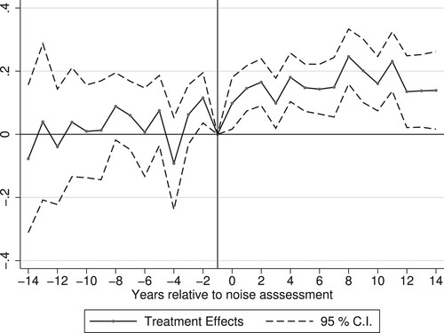
Figure 1 presents graphical evidence of the impact of the noise mitigation programme on property prices. The figure plots the results from an event study analysis in which the indicator for the treatment group has been interacted with a variable indicating time relative to assessment year. The difference in the year before the assessment serves as baseline. The post-assessment estimates in Figure 1 are all positive, thus implying an increase in the price of treated properties relative to control properties during this period. Pre-assessment differences fluctuate around zero and are generally statistically insignificant, which further supports the identifying assumption.

Figure 1. Event study graph.

Notes: The figure shows an event study graph based on a regression of the log of sales price on a full set of indicators for time relative to noise assessment interacted with the treatment group dummy variable. The estimate for the year before noise assessment is restricted to zero. The model includes municipality fixed effects, county-by-year fixed effects and property attributes. Plotted are the coefficients on the indicators together with their 95 percent confidence interval. Standard errors are two-way clustered by municipality and transaction year.

Figure 1 display some evidence of a relative price increase two years before assessment. Appendix Figure A1 therefore presents the results from an alternative event study regression in which the treatment group variable is interacted with event time dummies grouped into two-year periods. More observations are now used to estimate each treatment effect which potentially reduces the risk of noise. Reassuringly, this specification shows small and statistically insignificant pre-assessment estimates. Post-assessment effects remain positive and statistically significant.

Table 3 reports regression estimates from different versions of Equation (1(1) $\ln (P_{it})={\beta }_0+{\beta }_1{\mathrm{Noise}\mathrm{Mitigation}}_i+{\beta }_{2}Pos{t}_{it}+{\beta }_3{\mathrm{Noise}\mathrm{Mitigation}}_i\times Pos{t}_{it}+{\beta }_4{X}_i+{\theta }_t+e_{it}$(1) ). Column 1 is based on a specification with post- and treatment group indicators, county fixed effects and year-of-sale fixed effects. The estimate is statistically significant and reveals that the noise abatement programme raised property prices by 11 log points, or 12 percent. Estimate size and significance is robust to controlling for property attributes in column 2. Column 3 excludes property controls and replaces county fixed effects by municipality fixed effects. Identification is now based on comparisons of properties in the same municipality and sold the same year. The estimate is lower than those in columns 1 and 2 but remain precisely measured. Column 4 additionally includes property controls and reveals that the programme caused an increase in property values of 11 percent.

Table 3. Effect of noise mitigation on housing prices.

	(1)	(2)	(3)	(4)
Noise Mitigation × Post	0.111**	0.115***	0.096***	0.100***
	(0.045)	(0.043)	(0.033)	(0.032)
County FE	Yes	Yes	No	No
Housing Controls	No	Yes	No	Yes
Municipality FE	No	No	Yes	Yes
Observations	12,706	12,706	12,706	12,706
$R^2$	0.29	0.34	0.53	0.56

Note: The entries are the coefficient estimate of the difference-in-difference estimator in Equation (1(1) $\ln (P_{it})={\beta }_0+{\beta }_1{\mathrm{Noise}\mathrm{Mitigation}}_i+{\beta }_{2}Pos{t}_{it}+{\beta }_3{\mathrm{Noise}\mathrm{Mitigation}}_i\times Pos{t}_{it}+{\beta }_4{X}_i+{\theta }_t+e_{it}$(1) ). Dependent variable is the log of sales price. Standard errors two-way clustered by municipality and year of sale. * p<0.1, ** p<0.05, *** p<0.01

Table 4 investigates if the impacts are concentrated to certain properties. Each entry in columns 1–6 shows the estimate for a set of observations with scores either below or above the sample median of one of the housing quality indices. Effects are larger among properties with lower energy efficiency and exterior quality. Column 7 displays the results from a regression in which Equation (1(1) $\ln (P_{it})={\beta }_0+{\beta }_1{\mathrm{Noise}\mathrm{Mitigation}}_i+{\beta }_{2}Pos{t}_{it}+{\beta }_3{\mathrm{Noise}\mathrm{Mitigation}}_i\times Pos{t}_{it}+{\beta }_4{X}_i+{\theta }_t+e_{it}$(1) ) has been augmented with a triple interaction between the main treatment variable, ${\mathrm{Noise}\mathrm{Mitigation}}_i\times Pos{t}_{it}$, and the demeaned score on the housing quality index. This continuous specification also implies larger effects among lower quality dwellings.

Table 4. Heterogeneous effects by property attributes.

	Housing quality		Energy efficiency		Exterior quality		Continuous treatment
	(1)	(2)	(3)	(4)	(5)	(6)
	Low	High	Low	High	Low	High	(7)
Noise mitigation × Post	0.107**	0.098**	0.126***	0.056	0.148***	0.059	0.100***
	(0.044)	(0.038)	(0.038)	(0.049)	(0.042)	(0.043)	(0.032)
Noise mitigation × Post × Demeaned Housing Quality							−0.004** (0.002)
Housing Controls	Yes	Yes	Yes	Yes	Yes	Yes	Yes
Municipality FE	Yes	Yes	Yes	Yes	Yes	Yes	Yes
Observations	7,099	5,607	7,817	4,889	6,689	6,017	12,706
$R^2$	0.54	0.61	0.59	0.55	0.61	0.55	0.56

Note: Dependent variable is the log of sales price. Each entry in columns 1-6 reports the difference-in-differences estimate from Equation (1(1) $\ln (P_{it})={\beta }_0+{\beta }_1{\mathrm{Noise}\mathrm{Mitigation}}_i+{\beta }_{2}Pos{t}_{it}+{\beta }_3{\mathrm{Noise}\mathrm{Mitigation}}_i\times Pos{t}_{it}+{\beta }_4{X}_i+{\theta }_t+e_{it}$(1) ) on a subsample. The sample is bisected based on housing quality score below/above median in columns 1-2, energy efficiency score below/above median in columns 3-4 and exterior quality score below/above median in columns 5-6. Column 7 reports results for the full sample from a regression in which the main treatment variable has been interacted with the demeaned value of the score the housing quality index. Standard errors are two-way clustered by year of sale and municipality. * p<0.1, ** p<0.05, *** p<0.01

Properties with lower scores on the indices for energy efficiency, exterior and housing quality are more likely to have wooden facades, older facades and fewer windows with insulating glazing. As a result, they may have worse initial insulation. One explanation why the effect is larger for these properties is that they experience larger improvements in noise insulation and energy efficiency from noise mitigation than other property types do.

Table 5 tests the robustness of the main results by presenting alternative regression specifications. Column 1 reports the estimate from the property fixed effects model in Equation (2(2) $\ln (P_{it})={\beta }_3{\mathrm{Noise}\mathrm{Mitigation}}_i\times Pos{t}_{it}+{\gamma }_{1}Pos{t}_{it}+{\beta }_4{X}_i\times t+{\theta }_t+{\theta }_i+u_{it}$(2) ) on the repeated sales sample. The estimate indicates a positive and statistically significant effect that is close to the main difference-in-differences estimates. Column 2 reports the result from a property fixed effects model that only includes properties sold both before and after the assessment year. These observations constitute 30 percent of the full sample. The coefficient remains statistically significant and indicates a price increase of 12 percent. The repeated sales results thus provide some of the strongest support for the estimated effects on property prices.

Table 5. Robustness checks.

	(1)	(2)	(3)	(4)
	Repeat sale all	Repeat sale pre- & post	Time trends	Time trends
Noise Mitigation × Post	0.111***	0.116***	0.102**	0.055*
	(0.037)	(0.035)	(0.042)	(0.030)
Property FE	Yes	Yes	No	No
County FE	No	No	Yes	No
County trends	No	No	Yes	No
Municipality FE	No	No	No	Yes
Muncipality trends	No	No	No	Yes
Housing Controls	No	No	Yes	Yes
Observations	7,688	3,583	12,706	12,706
$R^2$	0.90	0.89	0.35	0.58

Note: Dependent variable is the log of sales price. Columns 1 and 2 present the results from the property fixed effect model in Equation (2(2) $\ln (P_{it})={\beta }_3{\mathrm{Noise}\mathrm{Mitigation}}_i\times Pos{t}_{it}+{\gamma }_{1}Pos{t}_{it}+{\beta }_4{X}_i\times t+{\theta }_t+{\theta }_i+u_{it}$(2) ). The specifications control for property attributes (interacted with linear time trends). The sample in column 1 consists of the properties sold multiple times. The sample in column 2 consists of properties sold multiple times and sold both before and after the noise assessment. Column 3 presents the results from the main equation augmented with county-specific trends. Column 4 presents the results from the main equation augmented with municipality-specific trends. The estimates in columns 3 and 4 are based on the main sample. Standard errors two-way clustered by municipality and year of sale. * p<0.1, ** p<0.05, *** p<0.01

The primary threat to the identification strategy is nonrandom treatment. For instance, it could be that noise mitigation was more likely to be provided in regions where the development of property values differed from others. The balancing tests in Table 2 provided evidence against the hypothesis that trends in property attributes differed between the treatment and control groups. It may still be that treatment is related to trends in unobserved price determinants. To assess this concern, columns 3 and 4 report estimates from models that include county and municipality-specific trends respectively. These trends pick up unobserved time-varying regional factors affecting property prices, such as neighbourhood demographics and other local amenities. Columns 3 and 4 indicate positive and statistically significant effects on prices. The estimate in column 4 is measured with less precision and is half the size of those from the main result. One reason could be the potential bias introduced by including regional time trends in the presence of a dynamic treatment effect (Wolfers 2006).

5.2. Additional sensitivity checks

This section subjects the main results to additional sensitivity checks. One potential concern for the identification strategy is that properties assessed by the SRA in the beginning of the programme were on different prices trends compared to properties assessed later. To address this issue, Column 1 of Table 6 reports the difference-in-differences estimate from the main equation with assessment-by-year fixed effects. These effects account for permanent differences between properties assessed different years. The estimate is statistically significant and close to the main results.

Table 6. Alternative treatment and control groups.

	(1)	(2)	(3)	(4)
	Assessment year FE	P-score 0.05–0.95	P-score 0.1–0.9	P-score 0.25–0.75
Noise Mitigation × Post	0.092***	0.098***	0.102***	0.121***
	(0.032)	(0.033)	(0.035)	(0.044)
Muncipality FE	Yes	Yes	Yes	Yes
Housing controls	Yes	Yes	Yes	Yes
Observations	12,706	11,434	10,164	6,343
$R^2$	0.57	0.57	0.57	0.53

Note: Dependent variable is the log of sales price. Column 1 presents results from the main equation augmented with assessment-by-year fixed effects. Columns 2–4 present the result from the main equation on samples that have been trimmed using the properties' propensity score for treatment group status. Standard errors two-way clustered by municipality and year of sale. * p<0.1, ** p<0.05, *** p<0.01

Another threat to identification is that treatment and control properties differ in terms of attributes and that these differences give rise to differential time trends. While the balancing tests in Table 2 provide evidence against this hypothesis, it may be that treated and control properties differed in terms of unobserved characteristics. I investigate this question by running the main equation on samples that have been trimmed using propensity score. These sample cuts omit properties with either very high or low probability of receiving noise mitigation and thus potentially restrict the comparison to more similar homes. I estimate the propensity scores from a logit model with the treatment indicator as dependent variable. The explanatory variables are county fixed effects and the property attributes. Column 2 presents the estimate based on observations with propensity scores within the 5th and 95th percentile. Columns 3 and 4 use observations with propensity scores on the 10th to 90th and 25th to 75th percentile interval respectively. All estimates are statistically significant and close to the main estimates. Taken together, the conclusions of the main results remain unchanged when restricting attention to these sets of observations.

Table 7 presents a series of falsification tests. Columns 1 and 2 show the results from a temporal placebo test in which the noise assessment year is brought forward one year for all observations. The sample consists of properties sold before the year of the actual assessment. The difference-in-differences estimates from this model test for a non-real treatment effect, why statistically significant estimates would be an issue. Reassuringly, the estimates are statistically insignificant, and magnitudes are small.

Table 7. Falsification tests.

	False assessment date		False predicted treatment		Only control group
	(1)	(2)	(3)	(4)	(5)	(6)
Noise Mitigation × Post	−0.001	−0.015	0.022	0.027
	(0.092)	(0.062)	(0.052)	(0.041)
Post					−0.014	−0.002
					(0.057)	(0.042)
Housing controls	Yes	Yes	Yes	Yes	Yes	Yes
County FE	Yes	No	Yes	No	Yes	No
Municipality FE	No	Yes	No	Yes	No	Yes
Observations	4,763	4,763	4,177	4,177	4,177	4,177
$R^2$	0.28	0.54	0.34	0.59	0.34	0.59

Note: Dependent variable is the log of sales price. Columns 1–2 present difference-in-differences estimates from Equation (1(1) $\ln (P_{it})={\beta }_0+{\beta }_1{\mathrm{Noise}\mathrm{Mitigation}}_i+{\beta }_{2}Pos{t}_{it}+{\beta }_3{\mathrm{Noise}\mathrm{Mitigation}}_i\times Pos{t}_{it}+{\beta }_4{X}_i+{\theta }_t+e_{it}$(1) ) with the assessment year brought forward one year for all observations. The sample consists of properties sold before their true assessment year. Columns 3-4 present difference-in-differences estimates from Equation (1(1) $\ln (P_{it})={\beta }_0+{\beta }_1{\mathrm{Noise}\mathrm{Mitigation}}_i+{\beta }_{2}Pos{t}_{it}+{\beta }_3{\mathrm{Noise}\mathrm{Mitigation}}_i\times Pos{t}_{it}+{\beta }_4{X}_i+{\theta }_t+e_{it}$(1) ) based on a sample of properties in the control group. Treatment status are assigned to the properties in the top 67 percent of the distribution of propensity treatment scores. Columns 5-6 present estimates on the post-assessment indicator in Equation (1(1) $\ln (P_{it})={\beta }_0+{\beta }_1{\mathrm{Noise}\mathrm{Mitigation}}_i+{\beta }_{2}Pos{t}_{it}+{\beta }_3{\mathrm{Noise}\mathrm{Mitigation}}_i\times Pos{t}_{it}+{\beta }_4{X}_i+{\theta }_t+e_{it}$(1) ) based on a regression using a sample of control properties only. Standard errors two-way clustered by municipality and year of sale.* p<0.1, ** p<0.05, *** p<0.01

Columns 3 and 4 present falsification tests based on a sample of control properties only. The properties are assigned pseudo-treatment status using their propensity score. The top 67 percent are classified as treated to mimic the share in the main sample. Again, a statistically significant estimate would be concerning. However, the estimates are both economic and statistically insignificant.

The main estimates would be biased if control properties were affected by the SRA's noise assessment. For instance, a notification of programme ineligibility could depress the property price in a subsequent sale. This concern is addressed in columns 5 and 6, which display the estimate on the post-indicator from a difference-in-difference model run only on control properties. The coefficient tests whether the average price of control properties sold in the same region and year differed depending on assessment status. A statistically significant coefficient would suggest that noise assessments affected control properties. However, results are small in magnitude and insignificant.

The SRA updated their noise assessments for some properties that already had received noise mitigation. The implementation year therefore predates the assessment year for 23 percent of the observations. The assessment year is missing for an additional 6 percent. I replaced the assessment year with the implementation year for these observations to produce the main results. Table 8 verifies that the results are robust to alternative imputation strategies.

Table 8. Estimates based on sample without imputed values.

	(1)	(2)	(3)	(4)	(5)	(6)
Noise Mitigation × Post	0.100***	0.067*	0.066*	0.114***	0.115***	0.120***
	(0.033)	(0.037)	(0.039)	(0.038)	(0.041)	(0.044)
Municipality FE	Yes	Yes	Yes	No	No	No
Property FE	No	No	No	Yes	Yes	Yes
Observations	11,973	9,722	8,989	7,256	5,797	5,365
$R^2$	0.57	0.57	0.58	0.89	0.89	0.89

Note: Dependent variable is the log of sales price. Columns 1–3 report the coefficient from the difference-in-difference model in Equation (1(1) $\ln (P_{it})={\beta }_0+{\beta }_1{\mathrm{Noise}\mathrm{Mitigation}}_i+{\beta }_{2}Pos{t}_{it}+{\beta }_3{\mathrm{Noise}\mathrm{Mitigation}}_i\times Pos{t}_{it}+{\beta }_4{X}_i+{\theta }_t+e_{it}$(1) ). Column 1 drops observations with missing assessment year, column 2 drops observations with implementation year predating assessment year and column 3 drops both types of observations. Columns 4–6 report the coefficient from the repeated sales model in Equation (2(2) $\ln (P_{it})={\beta }_3{\mathrm{Noise}\mathrm{Mitigation}}_i\times Pos{t}_{it}+{\gamma }_{1}Pos{t}_{it}+{\beta }_4{X}_i\times t+{\theta }_t+{\theta }_i+u_{it}$(2) ). Column 4 drops observations with missing assessment year, column 5 drops observations with implementation year predating assessment year and column 6 drops both types of observations. Standard errors two-way clustered by municipality and year of sale. * p<0.1, ** p<0.05, *** p<0.01

Columns 1 to 3 present estimates from the richest specification in Equation (1(1) $\ln (P_{it})={\beta }_0+{\beta }_1{\mathrm{Noise}\mathrm{Mitigation}}_i+{\beta }_{2}Pos{t}_{it}+{\beta }_3{\mathrm{Noise}\mathrm{Mitigation}}_i\times Pos{t}_{it}+{\beta }_4{X}_i+{\theta }_t+e_{it}$(1) ). The first column drops observations with missing assessment year, the second drops observations with implementation year predating assessment year and the third column drops both types of observations. The estimates are positive and statistically significant although those in columns 2 and 3 are smaller than in the main results. Columns 4 to 6 are based on the property fixed effects model and drop observations in an identical manner to columns 1 to 3. The estimates are statistically significant and close to the baseline repeated sales results.

Finally, I investigate whether taste-based sorting contribute to the estimated price effect. Improved environmental quality may attract individuals with higher preferences for peace and quiet, as proxied by their income. An influx of wealthier individuals may lead to neighbourhood gentrification and improvements in other local amenities that raise housing values (Banzhaf and McCormick 2012). I test for sorting effects by running Equation (1(1) $\ln (P_{it})={\beta }_0+{\beta }_1{\mathrm{Noise}\mathrm{Mitigation}}_i+{\beta }_{2}Pos{t}_{it}+{\beta }_3{\mathrm{Noise}\mathrm{Mitigation}}_i\times Pos{t}_{it}+{\beta }_4{X}_i+{\theta }_t+e_{it}$(1) ) with demographic characteristics of buyers as outcome variables. Table 9 shows little sign of meaningful shifts in demographics. Income in levels and logs remain stable with effect sizes less than one percent. Age at transaction is also unaffected. The estimate for years of education is statistically significant at the ten percent level but corresponds to less than two percent of the pre-assessment average in the treatment group. Although there may be more subtle changes undetectable in this sample, these results imply that sorting responses to noise mitigation were not large.

Table 9. Effect on noise mitigation on buyer characteristics.

	(1)	(2)	(3)	(4)
	Income	Log(Income)	Years of education	Age
Noise Mitigation × Post	−0.107	−0.009	0.195*	−1.373
	(7.127)	(0.111)	(0.117)	(0.839)
Housing Controls	Yes	Yes	Yes	Yes
Municipality FE	Yes	Yes	Yes	Yes
Observations	6,315	6,315	6,315	6,315
$R^2$	0.12	0.11	0.14	0.17
Mean	164.1	4.4	11.2	41.2

Note: The entries are the coefficient estimate of the difference-in-difference estimator in Equation (1(1) $\ln (P_{it})={\beta }_0+{\beta }_1{\mathrm{Noise}\mathrm{Mitigation}}_i+{\beta }_{2}Pos{t}_{it}+{\beta }_3{\mathrm{Noise}\mathrm{Mitigation}}_i\times Pos{t}_{it}+{\beta }_4{X}_i+{\theta }_t+e_{it}$(1) ). The dependent variable is indicated in the top of each column. The sample consists of properties for which buyer characteristics are available. Standard errors two-way clustered by municipality and year of sale. * p<0.1, ** p<0.05, *** p<0.01

6. Economic impact

This section uses the estimated property price appreciation and investment cost records to perform a rough calculation of the programme's costs and benefits. The analysis covers average impacts and the distribution of impacts across property types and income groups.

The average investment cost in the SRA dataset is 78,788 SEK, or $7,900 (in year 2017 prices). To account for the large heterogeneity in costs, this figure is calculated as the weighted average of the mean costs of facade insulation (24,689 SEK) and noise barriers (199,202 SEK), with weights given by the type's share in the treatment group. The calculations are based on 1,334 observations with valid cost records (non-missing cost amounts above 1,000 SEK). The Data Appendix provides more details about the costs.

Table 10. Comparison of average cost and benefits of the noise abatement programme.

	Effect (%)	Price gain	Investment cost	Net benefits	Gain-Funding Ratio
Upper bound	12.2	130	79	51	1.66
Lower bound	10.1	108	79	29	1.37

Note: All amounts are in 1,000 SEK and refer to year 2017 SEK.

The estimated impact of the programme on property prices ranges from 10.1 to 12.2 percent in the baseline model in Table 3. Using the pre-assessment average price of treated properties of 1.07 million SEK, these estimates translate to a nominal increase of 108,070 to 130,540 SEK (Table 10). Thus, the estimated net benefit of the programme ranges between 29,282 and 51,752 SEK. These figures correspond to a ratio of property price gain to investment funding of 1.4 to 1.7. Using the metric of property price capitalization, the benefits of the noise mitigation programme clearly exceeded the costs.

Because of different property price effects depending on housing quality, the average cost and benefits could mask important heterogeneity. I investigate this question by calculating property-level cost and benefits. I first calculate predicted percentage impacts from the coefficient estimates in column 7 of Table 4 and each property's score on the housing quality index. Second, I divide properties into four categories based on the quartiles of the housing quality score distribution and calculate the pre-assessment mean price for each category. I then multiply the mean price with the percentage impact to get the nominal price appreciation per property. Finally, I subtract the investment cost from the nominal benefit to obtain the net benefits per property.

The first four columns of Table 11 summarize these results for each category of the housing quality score distribution. The sample consists of the 1,334 observations with valid cost records. The investment costs for these observations are lower than for the full sample because almost all investments refer to a facade insulation. Average net benefits are larger among properties with worse quality. Net benefits in the lowest quality category are 50 percent higher than in the top category. This result is primarily due to higher price gains for properties with lower initial housing quality, as documented in Table 4.

Table 11. Benefits, costs and income by quartile of the housing quality index.

	Effect (%)	Price gain	Investment cost	Net benefits	Seller income
1st quartile	13.4	113	24	88	126
2nd quartile	11.1	108	29	80	130
3rd quartile	9.6	105	32	73	139
4th quartile	6.8	90	29	61	175
Observations	1,334	1,334	1,334	1,334	5,209

Note: All amounts are in 1,000 SEK and refer to year 2017 prices. Properties are divided according to the quartiles of the housing quality score distribution.

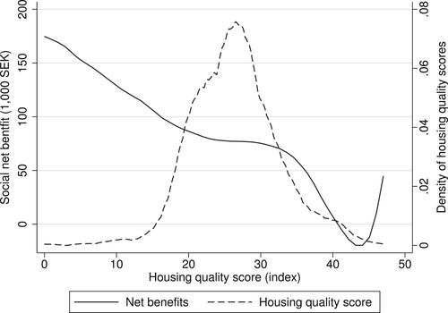
Figure 2 presents the relationship between net benefits and housing quality in greater detail. The solid line displays the estimated net benefits as a function of the housing quality score and the dotted line is the density of the housing quality scores. Net benefits are clearly declining in housing quality, particularly among homes with scores equal to or above the fourth quartile (30). This result reflects the smaller price effects for high quality properties previously documented. There appears to be some non-linearity in housing quality for scores above 45 but there are very few observations in that range.

Figure 2. Net benefits and housing quality.

Notes: The sample of 1,334 observations consists of transactions of treatment group properties with investment cost records above 1,000 SEK. Net benefits are calculated for each property from the two coefficients of column 7 in Table 4, the score on the housing quality index, the mean price per quartile of the housing quality score distribution and property-level investment costs. Net benefit is estimated by local polynomial. The density of housing quality is estimated by Epanechnikov kernel.

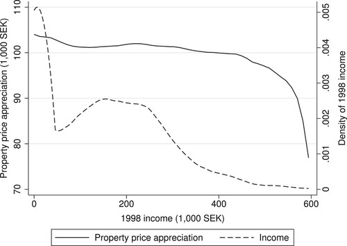
I further investigate disparities in programme benefits by comparing nominal house price appreciation across the income distribution of home sellers. This analysis disregards investment costs so the sample now consists of 5,209 transactions of properties in the treatment group with non-missing information on seller income. Column 5 of Table 11 reveal that mean income slightly increases with housing quality among the first three categories of the housing quality distribution. Income is significantly higher in the top category, indicating a selection of top earners into high quality properties. In Figure 3, the sold line plots estimated property price appreciation against seller income. The dotted line plots the income density. Price gains are evenly distributed over the income range where most households are but fall sharply for households earning more than 400,000 SEK. The gains for top earners are about 80 percent of those for the rest of the sample. Because of smaller price effects for high quality dwellings and selection of top earners into these properties, the distribution of benefits from the mitigation programme were progressive at the top of the income distribution.

Figure 3. Property price appreciation and seller income.

Notes: The sample of 5,169 observations consists of transactions of treatment group properties for which information on seller income is available and seller income is 600,000 SEK or less. Property price appreciations are calculated for each property from the two coefficients of column 7 in Table 4, the score on the housing quality index and the mean price per quartile of the housing quality score distribution. Property price appreciation is estimated by local polynomial. Income density is estimated by Epanechnikov kernel.

7. Conclusion

The study has used the housing market to evaluate a programme that provided instalments of noise barriers and facade insulation to properties exposed to high levels of noise. The evidence suggests that noise mitigation is causally related to increases in property values. The estimates reveal that the programme raised property prices by 10–12 percent on average. Accounting for the average investment cost, I estimate that the ratio of property price gain to investment funding of the programme was 1.4 –1.7. The return on investment is higher the lower is the initial quality of the property.

The results of this study have three main policy implications. First, the significant return of the programme constitute evidence to support noise mitigation measures in other settings. Second, the heterogeneous price impacts imply that mitigation measures provide largest benefits when targeted to dwellings with lower energy efficiency and exterior quality. Prioritizing measures to these property types is therefore likely to yield higher returns in future noise mitigation programmes. Third, the net benefit of the programme justifies alternative financing strategies. The SRA-funded mitigation measures yielded substantial dividend to property owners. Noise mitigation could still produce public health benefits large enough to motivate public spending on noise mitigation. This study documents private returns of the programme large enough to justify private (co-)financing of the measures, e.g. through low- or zero-interest loans to property owners.

Acknowledgments

I appreciate helpful comments from Niclas Krüger and Jan-Erik Swärdh.

Disclosure statement

This research evaluates a policy implemented by the Swedish Road Administration and its successor, the Swedish Transport Administration. The author has received funding from the Swedish Transport Administration for another research project.

Additional information

Funding

This work was supported by the Jan Wallanders och Tom Hedelius Foundation under Grant number P19-0010.

Notes

1 The population exposed to potentially harmful levels of noise exceeds 100 million in Europe (European Environmental Agency 2019)

2 Based on cost figures provided by the U.S. Department of Transportation https://www.fhwa.dot.gov/environment/noise/noise_barriers/inventory/ [accessed 10 October 2020].

3 Noise exposure has also been shown to disrupt cognitive behaviour and development (Clark and Paunovic 2018).

4 The programme was implemented through infrastructure bill 1996/97:53.

5 The equivalent noise level refers to the average sound pressure level during a specific time period, usually 24 hours, with weights given to sound occurring during different periods of the day. The maximum noise level refers to the maximum sound pressure level from a single event occurring during a specific time period, usually 24 hours.

6 Eight percent of the observations have missing values on the structural attributes due to matching failure. I impute these values using sample averages.

7 I omit apartment buildings because of the difficulty of identifying which units in a building that received a noise intervention. Only including transactions referring to a single property allows me to identify the type of property.

8 The main results remain the same on the sample that includes price outliers.

9 I take the average across residents in cases of multiple residents at a property in a year.

Appendix 1.

Details on investment cost

Investment cost in the SRA data set refers to either payments to contractors or reimbursement to property owners. About 40 percent of the treated properties records the investment cost. Almost half of the non-missing records are cost amounts of 0 and 1 SEK. It is uncertain what these values refer to and they are likely data errors. An additional 10 percent of the non-missing records are cost amounts between 1 and 1,000 SEK. These figures appear too low to represent the true construction costs. To minimize the risk of data error, I calculate averages using cost records exceeding 1,000 SEK. This means that calculations are based on 1,334 observations, which corresponds to 16 percent of the treatment group.

Figure A1. Grouped event study graph.

Notes: The figure shows an event study graph based on a regression of the log of sales price on a set of indicators for time relative to noise assessment interacted with the treatment group dummy variable. The indicators are grouped into two-year periods. The estimate for the two-year period before noise assessment is restricted to zero. The model includes municipality fixed effects, county-by-year fixed effects and property attributes. Plotted are the coefficients on the indicators together with their 95 percent confidence interval. Standard errors are two-way clustered by municipality and transaction year.

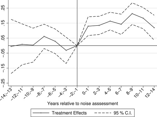
Figure A2. Annual noise assessments.

Notes: This figure shows the density of noise assessments per year, separately for the treatment and control groups.

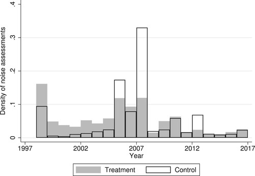
Table A1. Testing time to assessment and time to implementation.

	Years to assessment			Years to implementation
	(1)	(2)	(3)	(4)	(5)	(6)
Dwelling area	−0.001	0.001	0.001	0.000	0.001	0.001
	(0.001)	(0.001)	(0.001)	(0.001)	(0.001)	(0.001)
Construction year	0.005***	−0.000	0.001	−0.007***	−0.006***	−0.002
	(0.002)	(0.002)	(0.002)	(0.002)	(0.002)	(0.002)
Energy efficiency	0.080**	0.081***	0.065**	0.070	0.070	0.081**
	(0.033)	(0.030)	(0.028)	(0.047)	(0.043)	(0.041)
Exterior quality	−0.017	−0.005	−0.008	0.039	0.026	0.022
	(0.019)	(0.017)	(0.016)	(0.026)	(0.023)	(0.023)
Kitchen quality	−0.032	−0.027	−0.026	0.005	0.013	−0.008
	(0.023)	(0.021)	(0.020)	(0.034)	(0.031)	(0.029)
Sanitation quality	−0.007	−0.029	−0.007	−0.108***	−0.078**	−0.038
	(0.024)	(0.020)	(0.019)	(0.032)	(0.031)	(0.030)
Interior quality	−0.018	−0.002	0.007	0.115**	0.004	0.016
	(0.038)	(0.033)	(0.033)	(0.054)	(0.051)	(0.050)
County FE	No	Yes	No	No	Yes	No
Municipality FE	No	No	Yes	No	No	Yes
Observations	12,706	12,706	12,706	7,442	7,442	7,442
$R^2$	0.00	0.20	0.30	0.00	0.12	0.28

Note: In columns 1–3, the dependent variable is year of assessment relative to year 1998 and the sample consists of all observations. In columns 4-6, the dependent variable is year of implementation relative to year 1998 and the sample consists of observations in the treatment group. Standard errors are two-way clustered by municipality and year of sale. * p<0.1, ** p<0.05, *** p<0.01

The average cost of installing facade insulation is 24,689 SEK per property (median 18,673 SEK). This figure is based on 1,305 observations. The SRA calculates the per property cost of installing noise barriers by diving total investments costs by the number of properties deemed to have received a reduction in noise exposure levels. The average cost of installing noise barriers is 199,202 SEK per property (median 221,729 SEK). This figure is based on 29 observations.

I calculate the average investment cost of the programme as the weighted average of each type of mitigation measure, with weights given by the type's share in the treatment group. About 69 percent of observations in the treatment group receive facade insulation and 31 percent a noise barrier. The average investment cost of the programme thus amounts to $24,689\times 0.69+199,202\times 0.31=78,788$ SEK.

Appendix 2.

Figures

Appendix 3.

Tables

References

- Amundsen, Astrid H., Ronny Klæboe, and Gunn Marit Aasvang. 2011. “The Norwegian Façade Insulation Study: The Efficacy of Façade Insulation in Reducing Noise Annoyance Due to Road Traffic.” The Journal of the Acoustical Society of America 129 (3): 1381–1389.
- Andersson, Henrik, Lina Jonsson, and Mikael Ögren. 2010. “Property Prices and Exposure to Multiple Noise Sources: Hedonic Regression with Road and Railway Noise.” Environmental and Resource Economics 45 (1): 73–89.
- Baldauf, R., E. Thoma, A. Khlystov, V. Isakov, G. Bowker, T. Long, and R. Snow. 2008. “Impacts of Noise Barriers on Near-road Air Quality.” Atmospheric Environment 42 (32): 7502–7507.
- Bangjun, Zhang, Shi Lili, and Di Guoqing. 2003. “The Influence of the Visibility of the Source on the Subjective Annoyance Due to Its Noise.” Applied Acoustics 64 (12): 1205–1215.
- Banzhaf, H., and Eleanor McCormick. 2012. “Moving Beyond Cleanup.” In The Political Economy of Environmental Justice, 23–51.
- Basner, Mathias, and Sarah McGuire. 2018. “WHO Environmental Noise Guidelines for the European Region: a Systematic Review on Environmental Noise and Effects on Sleep.” International Journal of Environmental Research and Public Health 15 (3): 519.
- Bendtsen, H., L. Michelsen, and E. C. Christensen. 2011. “Noise Annoyance Before and After Enlarging Danish Highway.” In 6th Forum Acusticum, Aalborg, Denmark, Vol. 27.
- Billings, Stephen B., and Kevin T. Schnepel. 2017. “The Value of a Healthy Home: Lead Paint Remediation and Housing Values.” Journal of Public Economics 153: 69–81.
- Brown, Alan Lex, and Irene Van Kamp. 2017. “WHO Environmental Noise Guidelines for the European Region: a Systematic Review of Transport Noise Interventions and Their Impacts on Health.” International Journal of Environmental Research and Public Health 14 (8): 873.
- Clark, Charlotte, and Katarina Paunovic. 2018. “WHO Environmental Noise Guidelines for the European Region: A Systematic Review on Environmental Noise and Cognition.” International Journal of Environmental Research and Public Health 15 (2): 285.
- European Environmental Agency. 2019. Environmental Noise in Europe 2020. Technical Report. European Environmental Agency EEA Report 22.
- Gamper-Rabindran, Shanti, and Christopher Timmins. 2013. “Does Cleanup of Hazardous Waste Sites Raise Housing Values? Evidence of Spatially Localized Benefits.” Journal of Environmental Economics and Management 65 (3): 345–360.
- Gerarden, Todd D., Richard G. Newell, and Robert N. Stavins. 2017. “Assessing the Energy-efficiency Gap.” Journal of Economic Literature 55 (4): 1486–1525.
- Koster, Hans R. A., and Jos Van Ommeren. 2019. “Place-based Policies and the Housing Market.” Review of Economics and Statistics 101 (3): 400–414.
- Laszlo, H. E., E. S. McRobie, S. A. Stansfeld, and A. L. Hansell. 2012. “Annoyance and Other Reaction Measures to Changes in Noise Exposure–A Review.” Science of the Total Environment 435: 551–562.
- Münzel, Thomas, Tommaso Gori, Wolfgang Babisch, and Mathias Basner. 2014. “Cardiovascular Effects of Environmental Noise Exposure.” European Heart Journal 35 (13): 829–836.
- Nelson, Jon P. 2008. “Hedonic Property Value Studies of Transportation Noise: Aircraft and Road Traffic.” In Hedonic Methods in Housing Markets, 57–82. Springer.
- Nilsson, Mats E., and Birgitta Berglund. 2006. “Noise Annoyance and Activity Disturbance Before and After the Erection of a Roadside Noise Barrier.” The Journal of the Acoustical Society of America 119 (4): 2178–2188.
- Pirrera, Sandra, Elke De Valck, and Raymond Cluydts. 2010. “Nocturnal Road Traffic Noise: A Review on Its Assessment and Consequences on Sleep and Health.” Environment International 36 (5): 492–498.
- Pournazeri, Sam, and Marko Princevac. 2015. “Sound Wall Barriers: Near Roadway Dispersion Under Neutrally Stratified Boundary Layer.” Transportation Research Part D: Transport and Environment41: 386–400.
- Rossi-Hansberg, Esteban, Pierre-Daniel Sarte, and Raymond Owens III. 2010. “Housing Externalities.” Journal of Political Economy 118 (3): 485–535.
- Sørensen, M., Z. J. Andersen, R. B. Nordsborg, T. Becker, A. Tjønneland, K. Overvad, and O. Raaschou-Nielsen. 2013. “Long-term Exposure to Road Traffic Noise and Incident Diabetes: A Cohort Study.” Environmental Health Perspectives 121 (2): 217–222.
- Swedish Road Administration. 2001. Bullerskyddsåtgärder allmänna råd för Vägverket. Technical Report. Report 2001:88.
- Swedish Transport Administration. 2018. Fasadåtgärder som bullerskydd. Technical Report. Report 2018:142.
- Theising, Adam. 2019. “Lead Pipes, Prescriptive Policy and Property Values.” Environmental and Resource Economics 74 (3): 1355–1382.
- Van Kempen, Elise, Maribel Casas, Göran Pershagen, and Maria Foraster. 2018. “WHO Environmental Noise Guidelines for the European Region: a Systematic Review on Environmental Noise and Cardiovascular and Metabolic Effects: a Summary.” International Journal of Environmental Research and Public Health 15 (2): 379.
- Von Graevenitz, Kathrine. 2018. “The Amenity Cost of Road Noise.” Journal of Environmental Economics and Management 90: 1–22.
- Wolfers, Justin. 2006. “Did Unilateral Divorce Laws Raise Divorce Rates? A Reconciliation and New Results.” American Economic Review 96 (5): 1802–1820.
- World Health Organization. 2018. “Environmental Noise Guidelines for the European Region”.