
Abstract
In this paper, a partial dependent predator–prey system with multiple delays is investigated. By choosing τ1, τ2 and τ3 as bifurcating parameters, we show that Hopf bifurcations occur. In addition, by using theory of functional differential equation and Hassard's method, explicit algorithms for determining the direction of the Hopf bifurcation and the stability of bifurcating periodic solutions are derived. Finally, numerical simulations are performed to support the analytical results, and the chaotic behaviors are observed.
1. Introduction
Since the work of Volterra, the Lotka–Volterra system has been extensively investigated. A classical Lotka–Volterra system can be modeled by the following system:
In the present paper, we devote our attention to the bifurcating phenomenons of the predator–prey system with three delays. So the system is not only more complicated, but also more close to the actuality. We described the system by
This paper is organized as follows: in Section 2, we investigate the effect of the time delays τ1, τ2 and τ3 on the stability of the positive equilibrium of system (3). In Section 3, we derive the direction and stability of the Hopf bifurcation by using normal form and central manifold theory. Finally in Section 4, numerical simulations are carried out to illustrate the theoretical prediction and to explore the complex dynamics including chaos.
2. Stability analysis and Hopf bifurcation
It is easy to see that system (3) has a unique positive equilibrium provided that the following condition is satisfied:
where
Let
, and still denote by
, system (3) can be written as
where
We then obtain the linearized system
The corresponding characteristic equation is
Case (a1) , Equation (4) becomes
All roots have negative real parts if and only if
Theorem 2.1
For the interior equilibrium point E* is locally asymptotically stable if conditions (H*) and (5) hold.
Case (b1) .
Theorem 2.2
For assume that (H*) and
hold, the interior equilibrium point E* is locally asymptotically stable for
and it undergoes the Hopf bifurcation at
given by
Proof On substituting , the characteristic equation (4) becomes
Case (b2) .
Theorem 2.3
For assume that (H*) and
hold, the interior equilibrium point E* is locally asymptotically stable for
and it undergoes the Hopf bifurcation at
given by
The proof is similar as in case (b1).
Case (b3) .
Theorem 2.4
For assume that (H*) and
hold, the interior equilibrium point E* is locally asymptotically stable for
and it undergoes the Hopf bifurcation at
given by
The proof is similar as in case (b1).
Case (c1) is fixed in the interval
and τ1>0.
Theorem 2.5
Let , τ3=0 and
if (H*) holds, then the equilibrium E* is asymptotically stable for
and system (3) undergoes Hopf bifurcation at E* when
, where
Proof We know is in its stable interval and τ1 is considered as a parameter. Let
be a root of Equation (4). Separating real and imaginary parts leads to
Without going into detailed analysis with Equation (13), it is assumed there exists at least one real positive root ω12. Now Equation (12) can be written as
Case (c2) is fixed in the interval
and τ2>0.
Theorem 2.6
Let and
if (H*) holds, then the equilibrium E* is asymptotically stable for
and system (3) undergoes Hopf bifurcation at E* when
, where
The proof is similar as in case (c1).
Case (c3) is fixed in the interval
and τ1>0.
Theorem 2.7
Let and
if (H*) holds, then the equilibrium E* is asymptotically stable for
and system (3) undergoes Hopf bifurcation at E* when
, where
The proof is similar as in case (c1).
Case (c4) is fixed in the interval
and τ3>0.
Theorem 2.8
Let and
if (H*) holds, then the equilibrium E* is asymptotically stable for
and system (3) undergoes Hopf bifurcation at E* when
, where
The proof is similar as in case (c1).
Case (c5) is fixed in the interval
and τ2>0.
Theorem 2.9
Let and
if (H*) holds, then the equilibrium E* is asymptotically stable for
and system (3) undergoes Hopf bifurcation at E* when
, where
is a root of the corresponding characteristic equation and
The proof is similar as in case (c1).
Case (c6) is fixed in the interval
and τ3>0.
Theorem 2.10
Let , τ1=0 and
if (H*) holds, then the equilibrium E* is asymptotically stable for
and system (3) undergoes Hopf bifurcation at E* when
, where
The proof is similar as in case (c1).
Case (d1) τ2 and τ3 are fixed in the interval and
, τ1>0.
Theorem 2.11
Let ,
if (H*) holds, then the equilibrium E* is asymptotically stable for
and system (3) undergoes Hopf bifurcation at E* when
, where
Proof We know τ2, τ3 are in its stable interval and τ1 is considered as a parameter. Let be a root of Equation (4). Separating real and imaginary parts leads to
Without going into detailed analysis with Equation (22), it is assumed there exists at least one real positive root ω14. Now Equation (21) can be written as
Case (d2) τ1 and τ3 are fixed in the interval ,
and τ2>0.
Theorem 2.12
Let ,
and
if (H*) holds, then the equilibrium E* is asymptotically stable for
and system (3) undergoes Hopf bifurcation at E* when
, where
The proof is similar as in case (d1).
Case (d3) τ1 and τ2 are fixed in the interval ,
and τ3>0.
Theorem 2.13
Let ,
and
if (H*) holds, then the equilibrium E* is asymptotically stable for
and system (3) undergoes the Hopf bifurcation at E* when
, where
The proof is similar as in case (d1).
3. Direction and stability of the Hopf bifurcation
In this section, we show that system (3) undergoes a Hopf bifurcation for different combinations of τ1, τ2 and τ3 satisfying sufficient conditions as described. By using the method based on the normal form theory and the center manifold theory introduced by Hassard, Kazarinoff, andWan (Citation1981), we study the direction of bifurcations and the stability of bifurcating periodic solutions. Without loss of generality, these properties are studied for variable τ2 as parameter and are fixed. Let
,
is described in Equation (18), then the Hopf bifurcation occurs at μ=0. Assume that
where
. Now we rescale the time by
, for convenience,
are still written as x(t), y(t), then system (3) can be written as
where
respectively, the nonlinear terms f1 and f2 are
The delayed system can be written in the functional form as
By the Riesz representation theorem, there exists a matrix whose components are bounded variation functions
such that
where choosing
For
, define
and
where
Hence, Equation (3) can be rewritten as
where
and
For
define A(0)=A and the adjoint operator A* of A as
where ηT is the transpose of the matrix η.
For and
, in order to normalize the eigenvectors of operator A and adjoint operator A*, we define a bilinear inner product
where
.
Since are eigenvalues of A, they will also be the eigenvalues of A*. The eigenvectors of A and A* are calculated corresponding to the eigenvalues
and
.
lemma 3.1
is the eigenvector of A corresponding to
;
is the eigenvector of A* corresponding to
and
where
Following the algorithms explained in Hassard,Kazarinoff, and Wan (1981), which is used to obtain the properties of Hopf bifurcation:
where
We know
and
are constant vectors.
Thus, we can compute the following quantities:
These expressions give a description of the bifurcating periodic solutions in the center manifold of system (3) at critical values
, whereas,
which can be stated as follows:
(i) μ2 gives the direction of the Hopf bifurcation: if
, the Hopf bifurcation is supercritical (subcritical).
(ii) β2 determines the stability of the bifurcating periodic solution, the periodic solution is stable (unstable) if
(iii) T2 denotes the period of bifurcating period solutions, if T2>0 (T2<0), the period increases (decrease).
4. Numerical simulations
To demonstrate the algorithm for determining the existence of the Hopf bifurcation in Section 2 and the direction and stability of the Hopf bifurcation in Section 3, we carry out numerical simulations on a particular case of Equation (3) in the following form.
We can see from (a) that E* is asymptotically stable at and
, while E* loses its stability and the Hopf bifurcation occurs at
and
, see (b). Then using the algorithm derived in Section 3, we obtain that
, we know that the Hopf bifurcation is supercritical, the bifurcating periodic solution is stable and the period increases. Whereas, at
and
it loses stability and a chaotic solution occurs (see (a)). In (b), the largest Lyapunov exponent diagram is plotted for variable τ1 when τ2=5.0 and τ3=2.1, it is easy to know when τ1>2.6, the Lyapunov exponent is almost positive, then the chaotic solutions occur. From (a), the largest Lyapunov exponent diagram is plotted for variable τ2 when τ1=2.7 and τ3=2.1, it is easy to know when
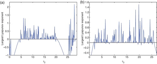
, the Lyapunov exponent is almost positive, then the chaotic solutions occur. Similarity, from (b), the largest Lyapunov exponent diagram is plotted for variable τ3 when τ1=2.7 and τ2=5.0, it is easy to know when
the Lyapunov exponent is almost positive, then the chaotic solutions occur.
Figure 1. (a) E* is asymptotically stable equilibrium at τ1=1.3, τ2=2.6 and τ3=0.085; (b) E* loses stability and Hopf bifurcation occurs at τ1=2.1, τ2=4.1 and τ3=0.3.
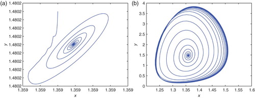
Figure 2. (a) E* loses stability and a chaotic solution occurs at τ1=2.7, τ2=5.0 and τ3=2.1; (b) the largest Lyapunov exponent diagram of system (4.1) for variable τ1 at τ2=5.0 and τ3=2.1.
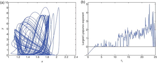
Figure 3. (a) The largest Lyapunov exponent diagram of system (4.1) for variable τ2 at τ1=2.7 and τ3=2.1; (b) for a variable τ3 at τ1=2.7 and τ2=5.0.
5. Conclusions
In this paper, we investigate the effect of the time delays τ1, τ2 and τ3 on the stability of the positive equilibrium of the system (3), and derive the direction and stability of the Hopf bifurcation. Numerical simulations are carried out to illustrate the theoretical prediction and to explore the complex dynamics including chaos.
Acknowledgements
We are grateful to the reviewers for their valuable comments and suggestions which have led to an improvement of this paper. This research is supported by the National Natural Science Foundation of China (No. 11061016).
REFERENCES
- Faria, T., & Magalhaes, L. (1995). Normal form for retarded functional differential equations and applications to Bogdanov–Takens singularity. Journal of Differential Equations, 122, 201–224. doi: 10.1006/jdeq.1995.1145
- Hassard, B., Kazarinoff, N., & Wan, Y. H. (1981). Theory and applications of Hopf bifurcation. London mathematical society lecture note series (Vol. 41). Cambridge: Cambridge University Press.
- Jin, Z., & Ma, Z. (2002). Stability for a competitive Lotka–Volterra system with delays. Nonlinear Analysis, 52, 1131–1142.
- Saito, Y. (2002). The necessary and sufficient condition for global stability of a Lotka–Volterra cooperative or competition system with delays. Journal of Mathematical Analysis and Applications, 268, 109–124. doi: 10.1006/jmaa.2001.7801
- Song, Y., Han, M., & Peng, Y. (2004). Stability and Hopf bifurcation in a competitive Lotka–Volterra system with two delays. Chaos, Solitons and Fractals, 22, 1139– 1148. doi: 10.1016/j.chaos.2004.03.026
- Song, Y., Peng, Y., & Wei, J. (2008). Bifurcation for a predator–prey system with two delays. Journal of Mathematical Analysis and Applications, 337, 446–479. doi: 10.1016/j.jmaa.2007.04.001
- Sun, C., Lin, Y., & Han, M. (2006). Stability and Hopf bifurcation for an epidemic disease model with delay. Chaos, Solitons and Fractals, 30, 204–216. doi: 10.1016/j.chaos.2005.08.167
- Tang, X., & Zhou, X. (2003). Global attractivity of non-autonomous Lotka–Volterra competition system without instantaneous negative feedback. Journal of Differential Equations, 192, 502–535. doi: 10.1016/S0022-0396(03)00042-1
- Yan, X., & Chu, Y. (2006). Stability and bifurcation analysis for a delayed Lotka–Volterra predator–prey system. Journal of Computational and Applied Mathematics, 196, 198–210. doi: 10.1016/j.cam.2005.09.001
- Zhang, J., Jin, Z., Yan, J., & Sun, G. (2009). Stability and Hopf bifurcation in a delayed competition system. Nonlinear Analysis, 70, 658–670. doi: 10.1016/j.na.2008.01.002