A state-space approach to mathematical modeling and parameters identification of vehicle frontal crash

Abstract

In this paper a state-space estimation procedure that relies on the time-domain analysis of input and output signals is used for mathematical modeling of vehicle frontal crash. The model is a double-spring–mass–damper system, whereby the front mass and real mass represent the chassis and the passenger compartment, respectively. It is observed that the dynamic crash of the model is closer to the dynamic crash from experimental when the mass of the chassis is greater than the mass of the passenger compartment. The dynamic crash depends on pole placement and the estimated parameters. It is noted that when the poles of the model are closer to zero, the dynamic crash of the model is far from the dynamic crash from the experimental data. The stiffness and damping coefficients play an important role in the dynamic crash.

Keywords:

• modeling
• vehicle frontal crash
• parameter identification
• state-space representation

1. Introduction

The car crash test is usually performed in order to ensure safe design standards in crashworthiness, the ability of a vehicle to be plastically deformed and yet maintain a sufficient survival space for its occupants during crash scenario. Nowadays, due to advanced research in computer simulation software, simulated crash tests can be performed beforehand the full-scale crash test. Therefore, cost associated with real crash test can be reduced.

Vehicle crashworthiness can be evaluated in four distinct modes: frontal, side, rear and rollover crashes.

System identification concerns the construction and validation of mathematical models of dynamical systems from experimental input/output data. In experiments the system reveals information about itself in terms of input and output measurements. System identification is routinely used in industry as a tool for plant modeling.

There are available solutions for the identification of mathematical models based on experimental test procedures. One of the most convenient and accessible solution is to use the system identification toolbox (Mathworks, R2013b).

In addition to the general use, the system identification toolbox is also commonly used for creating models of vibrating mechanical systems (Skullestad & Hallingstad, 1998; Weber & Feltrin, 2010). The system identification toolbox is largely based on the work of Ljung (1999) and implements common techniques used in system identification. There is substantial literature on system identification (Ljung & Glad, 1994). The toolbox aids the user to fit both linear and nonlinear models to measured data sets known as black box modeling (Marzbanrad & Pahlavani, 2011b). The system identification problem is to determine the unknown system characteristics such as mass, stiffness and damping parameters using system responses. In the work of Khattab (2010), an investigation of an adaptable crash energy management system to enhance vehicle crashworthiness was carried out. The author performed a system identification algorithm for vehicle lumped parameter model in crash analysis using a genetic algorithm procedure, an effective procedure for optimizing errors between experimental data and calculated data obtained analytically. Also a systematic investigation of vehicle frontal crash was conducted using the lumped-parameter model by Pawlus, Nielsen, Karimi, and Robbersmyr (2011). Pawlus, Robbersmyr, and Karimi (2011) proposed a mathematical model to estimate the maximum occupant deceleration, which is one of the main tasks in the area of crashworthiness study by a Kelvin model which contains a mass together with a spring and damper connected in parallel. An application of physical models composed of springs, dampers and masses joined together in various arrangements for simulating a real car collision with a rigid pole was presented by Pawlus, Karimi, and Robbersmyr (2011).

Marzbanrad and Pahlavani (2011a) presented an overview of the kinematic and dynamic relationships of a vehicle in a collision, whereby the work was to identify the parameters of the vehicle crash model using experimental data set. Munyazikwiye, Karimi, and Robbersmyr (2013) estimated the physical parameters of a frontal car crash using the eigensystem realization algorithm and curve-fitting approaches. Marzbanrad and Pahlavani (2011c) investigated and analyzed a lumped-parameter modeling in frontal crash in five degrees of freedom, and the response of occupant during the impact was investigated.

The types of available models are low-order process models, transfer functions, state-space models, linear models with static nonlinearities, nonlinear autoregressive models, etc. The identification tasks are divided into separate parts. After creating an identification and validation data set, the data are pre-processed. Identification is initialized by selecting and setting up the proper model type. Finally, the models can be validated using numerous techniques such as comparing model response with measurement data, step response and a pole-zero plot.

The aim of the identification process is to identify the contents of matrices A, B and C given the input and output data set. The Matlab system identification toolbox offers two estimation methods for state-space models:

• Subspace identification

• Iterative prediction-error minimization method

The matrix is called the (dynamical) system matrix. It describes the dynamics of the system (as completely characterized by its eigenvalues). is the input matrix which represents the linear transformation by which the deterministic inputs influence the next state, is the output matrix which describes how the internal state is transferred to the outside world in the measurements y_k. The term with the matrix is called the direct feedthrough term. In continuous time systems this term is most often 0.

In this paper, the state-space of the model under study was obtained and the physical parameters (stiffness and damping coefficients) were extracted from the dynamical system matrix . The model was finally validated by the experimental data. The results from the model are much closer to the real crash scenario. The results show that a vehicle with the chassis heavier than the passenger compartment experiences less dynamic crash. Therefore, care should be taken by car designer as far as the ratios (with respect to the total mass of the car) of the chassis and passenger compartment are concerned.

The novelty of the approach used in this paper is that it is less computational as compared with the previous approaches, like eigensystem realization and curve-fitting techniques, in the literature and the simulation results are much closer to the experimental results.

2. Vehicle crash experimental test

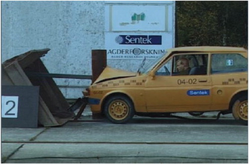
The real vehicle crash experiment was conducted on a typical mid-speed vehicle to pole collision. Its elaboration was the initiative of Robbersmyr (2004). A test vehicle was subjected to impact with a vertical and rigid cylinder. The acceleration field was 100 m long and had two anchored parallel pipelines. The vehicle was steered using those pipelines that were bolted to the concrete runaway. The setup scheme is shown in Figure 1. During the test, the acceleration was measured in three directions (x – longitudinal, y – lateral and z – vertical) together with the yaw rate from the center of gravity of the car. Using normal speed and high-speed video cameras, the behavior of the safety barrier and the test vehicle during the collision was recorded. The initial velocity of the car was 35 km/h, and the mass of the vehicle (together with the measuring equipment and dummy) was 873 kg. The obstruction was constructed with two steel components – a pipe filled with concrete and a baseplate mounted with bolts on a foundation. The car undergoing the deformation is shown in Figure 2. The accelerometer is located at the mass center of gravity of the vehicle in the passenger compartment. Since we are interested in the frontal crash, only the measured acceleration in the longitudinal direction is considered in this study. The acceleration data are imported and processed in Matlab for analysis. The deformation of the vehicle is obtained by integrating twice the acceleration signal.

Figure 1. Vehicle crash experimental setup (Robbersmyr, 2004).

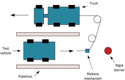
Figure 2. Vehicle undergoing deformation (Robbersmyr, 2004).

3. Mathematical modeling

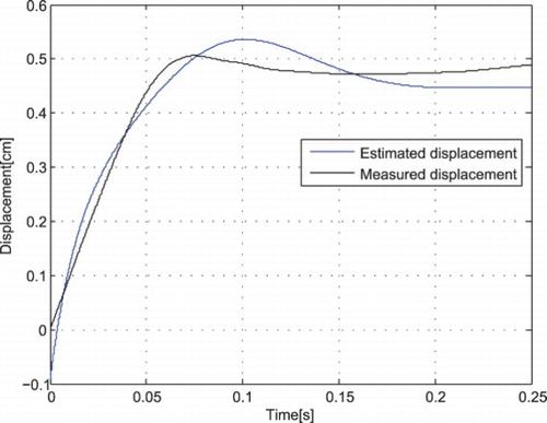
The experimental data were first imported in the Matlab workspace and processed for being suitable for the identification of the model. The measured acceleration was twice integrated to obtain the measured displacement signal. The processed data were further imported into a system identification toolbox. A transfer function model and a state-space canonica form were thereafter obtained.

Figure 3 shows the measured input–output signals and simulated output. The transfer function from the experimental data is as follows:

Figure 3. Measured and estimated outputs.

The estimated state-space model of order 4 is as follows:

Mathematical models describe the dynamic behavior of a system as a function of time. During frontal crash, the vehicle is subjected to an impulsive force caused by the obstacle. The model for vehicle crash simulates a rigid barrier impact of a vehicle where m₁ and m₂ represent the frame rail (chassis) and passenger compartment masses, respectively.

Parameters to be estimated are springs k₁ and k₂, dampers c₁ and c₂, as shown in Figure 4. When the vehicle impacts on a rigid barrier, the two masses will experience an impulsive force during collision. The method for solving the impact responses of the two masses is adapted from the method used in the free vibration analysis of a two degrees of freedom damped system (Huang, 2002).

Figure 4. A double-spring–mass–damper model.

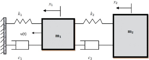
The dynamic equations of the double mass–spring–damper model are shown in Equation (3).

or

From Equation (4) a transfer function between u(t) and x₂(t) is derived and given in Equation (5).

with

The state-space canonical form representation from this transfer function is

with

The physical parameters are embedded in the state matrix. Therefore by inspection, the identified parameters are obtained by comparing the two state matrices in Equation (2) and in Equation (6), which are summarized in the following:

A summary of estimated parameters considering different cases is shown in Table 1. Only real values are considered.

Table 1.  Parameters estimation.

		Estimated Parameters
Cases	Solution no.	k1(N/m)	k2(N/m)	c1(N s/m)	c2(N s/m)
Case1:m1=1/3 mt	1	3498.37	640,808	22,989	9440
m2=2/3 mt	2	15,324.66	6293.37	5247	96,1212.45
Case2:m1=2/3 mt	1	7720.9	440,070	33,306.4	13,746.15
m2=1/3 mt	2	11,102.14	33,162.72	458,205	1,320,210
Case3:m1=1/4 mt	1	475.68	606,207.28	20,541.68	8419.68
m2=3/4 mt	2	15,406.26	6314.76	634.24	808,276.38
Case4:m1=3/4 mt	1	6734.92	337,670.38	36,588.11	15,115.54
m2=1/4 mt	2	9147	3778.88	26,939.66	1,350,681.54

4. Simulation results

Four different cases were considered for simulation of vehicle frontal crash. The solution of Equation (7) is not unique. Four solutions for each parameter were found, two real and two complex conjugate solutions. For the physical system, only real values have meaning. Therefore the complex solutions were neglected in the development of the model. A summary of estimated real valued parameters is shown in Table 1.

Case 1: (m₁<m₂). One has that and .

Solution of Equation (7) is as follows:

Taking c₁=22987 N s/m; k₁=3498.37 N/m; c₂=9770.06 N s/m;  N/m; the state-space canonical form is and

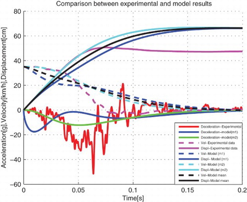
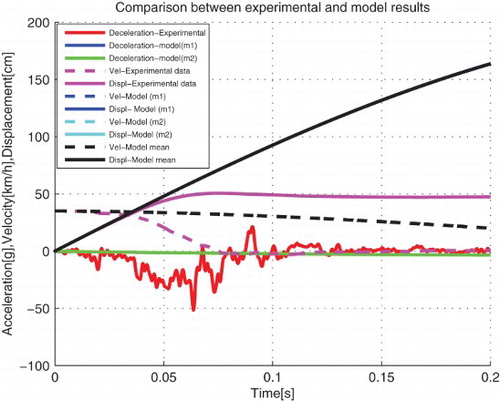
From Figure 5, the dynamic crash of m₂ is 66.55 cm which is the displacement of the passenger compartment. Therefore this model cannot represent the vehicle crash scenario. It is observed that the time for dynamic crash is longer than that for the real crash (i.e. 0.14 s instead of 0.078 s). The dynamic crash of the chassis represented by m₁ is more or less equal to that of the passenger compartment – a difference of 0.43 cm is observed and the time of crash is larger compared with that from the real crash and that from the passenger compartment (i.e. 0.17 s). The model where the chassis is a third of the car cannot represent the crash scenario.

Figure 5. Comparative analysis between vehicle crash test and model results for m₁=⅓m_t.

Taking c₁=5247.56 N s/m;  N/m;  N s/m; k₂=6293.37 N/m and

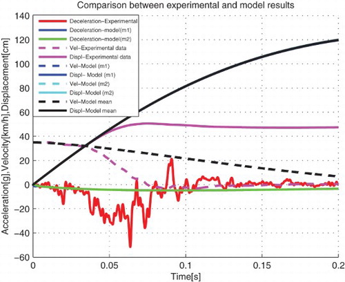
From Figure 6 the value of dynamic crash of the passenger compartment as represented by mass m₂ is very high and cannot be observed from the response graph, i.e. tends to ∞, resulting in a critically stable system because of a pole at zero. Therefore, this model cannot represent the vehicle crash scenario because the deformation of the car cannot tend to ∞. The time of crash is not observed because the velocity never crosses zero as an indication of maximum time of crash. Therefore, the physical parameters obtained for this model are not of much interest.

Figure 6. Comparative analysis between vehicle crash test and model results for m₂=⅓m_t.

Case 2: (m₁>m₂). One has that and

Solution of Equation (7) is as follows:

Taking c₁=33306.4 N s/m; k₁=7720.9 N/m;  N s/m;  N/m; the state-space canonical form is and

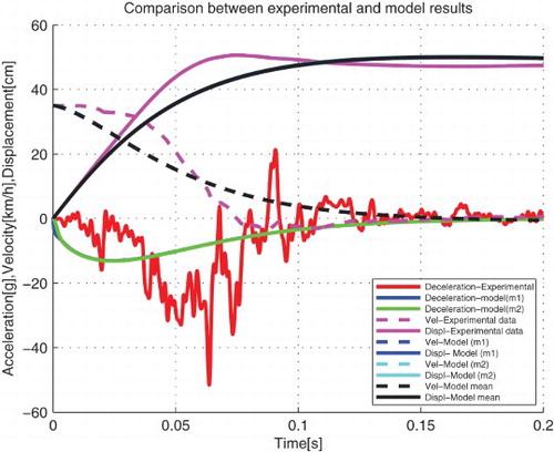
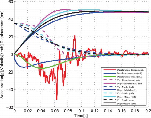
From Figure 7, the dynamic crash of the passenger compartment is 52.92 cm and the time for dynamic crash decreases as compared with the previous case, that is, from 0.14 to 0.11 s. The dynamic crash of the chassis is 51.05 cm and occurs after 0.16 s. Therefore for this case, the model can represent the vehicle crash scenario because the dynamic crash is much closer to that obtained from the experimental data.

Figure 7. Comparative analysis between vehicle crash test and model results for m₁=¼m_t.

Taking  N s/m;  N/m; c₂=1320210 N s/m; k₂=458205 N/m and

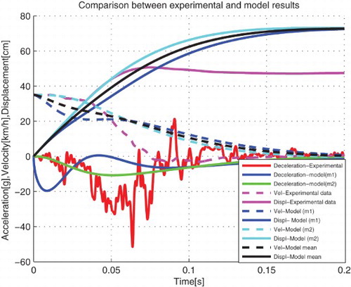
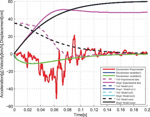
From Figure 8, the dynamic crash of the passenger compartment is 50.16 cm and the time for dynamic crash increases as compared with the previous case, that is, from 0.14 to 0.16 s. The dynamic crash of the chassis is 49.82 cm and occurs after 0.16 s. Therefore for this case, the model can represent the vehicle crash scenario because the dynamic crash is much closer to that obtained from the experimental data.

Figure 8. Comparative analysis between vehicle crash test and model results for m₂=¼m_t.

Case 3: (m₁<m₂). One has that and .

Solution of Equation (7) is as follows: Taking  N s/m; k₁=47.68 N/m;  N s/m;  N/m; the state-space canonical form is and

From Figure 9, the dynamic crash of m₂ is 73.07 cm which is the displacement of the passenger compartment. Therefore, this model cannot represent the vehicle crash scenario. It is observed that the time for dynamic crash is longer than that for the real crash (i.e. 0.17 s instead of 0.078 s). The dynamic crash of the chassis represented by m₁ is more or less equal to that of the passenger compartment – a difference of 0.62 cm is observed and the time of crash is same as that of passenger compartment and larger as compared with that from the real crash (i.e. 0.17 s). The model where the mass of the chassis is a quarter of that of the car cannot represent the crash scenario.

Figure 9. Comparative analysis between vehicle crash test and model results for m₂=¼m_t.

Taking c₁=634.24 N s/m;  N/m;  N s/m; k₂=6314.76 N/m; the state-space canonical form is and

The dynamic crash and time of crash represented in Figure 10 are similar to those in Figure 7. The value of dynamic crash of the passenger compartment as represented by mass m₂ is very high and cannot be observed from the response graph, i.e. tends to ∞. Therefore, this model cannot represent the vehicle crash scenario.

Figure 10. Comparative analysis between the vehicle crash test and model results for m₂=¼m_t.

Case 4: (m₁>m₂). One has that and .

Solution of Equation (7) is as follows: Taking  N s/m; k₁=6734.92 N/m;  N s/m;  N/m; the state-space canonical form is and

From Figure 11, the dynamic crash of the passenger compartment is 50.48 cm and the time for dynamic crash decreases as compared with the previous case, that is, from 0.14 to 0.11 s. The dynamic crash of the chassis is 48.14 cm and occurs after 0.16 s. Therefore for this case, the model can represent the vehicle crash scenario because the dynamic crash is much closer to that obtained from the experimental data.

Figure 11. Comparative analysis between the vehicle crash test and model results for m₂=¼m_t.

Taking  N s/m; k₁=9147.03 N/m;  N s/m; k₂=3778.88 N/m; the state-space canonical form is and

From Figure 12 the dynamic crash of the passenger compartment m₂ is 60.24 cm and the time for dynamic crash is 0.24 s. The dynamic crash and time of crash of chassis are same as those of the passenger compartment. This case cannot represent the vehicle crash scenario because the dynamic crash is much diverging from the real vehicle crash.

Figure 12. Comparative analysis between vehicle crash test and model results for m₂=¼m_t.

A summary of main results is shown in Table 2. The parameter values depend on the value of mass m₂ taken into consideration.

Table 2.  Dynamic crash and time of crash comparison.

CmExp (cm)	Tm−Exp (s)	Solution no.1	Masses	Cm (cm)	Tm (s)	Solution no.2	Masses	Cm (cm)	Tm (s)
50.63	0.075	Case1:m1=1/3 mt	m2	66.55	0.14	Case1:m1=1/3 mt	m2	∞	–
		m2=2/3 mt	m1	66.13	0.19	m2=2/3 mt	m1	∞	–
		Case2:m1=2/3 mt	m2	52.92	0.11	Case2:m1=2/3 mt	m2	50.16	0.16
		m2=1/3 mt	m1	51.05	0.16	m2=1/3 mt	m1	49.82	0.15
		Case3:m1=1/4 mt	m2	73.07	0.17	Case3:m1=1/4 mt	m2	∞	–
		m2=3/4 mt	m1	72.45	0.17	m2=3/4 mt	m1	∞	–
		Case4:m1=3/4 mt	m2	50.48	0.11	Case4:m1=3/4 mt	m2	60.24	0.24
		m2=1/4 mt	m1	48.14	0.16	m2=1/4 mt	m1	60.24	0.24

The stiffness coefficients which result in a closer vehicle crash reconstruction are found to be k₁=74681 N/m, k₂=45821 N/m and the damping coefficients are: c₁=18176 N s/m, c₂=11196 N s/m in case 4, where the dynamic crash of the passenger compartment is equal to 49.8 cm and occurs after 0.11s (see Figures 8, 9 and 12).

When the mass of the chassis is greater than that of the passenger compartment, the results from the model are closer to the expected values. For example,

• When and , the identified parameters are: k₁=6734.92 N/m,  N/m,  N s/m and  N s/m. The dynamic crash of the chassis is 48.14 and the dynamic crash of the passenger compartment is 50.48 cm which is closer to 50.68 cm (the dynamic crash from the real vehicle crash).

• When and , the identified parameters are:  N/m,  N/m, c₁=4558205 N s/m and c₂=1320410 N s/m. The dynamic crash of the chassis is 49.82 and the dynamic crash of the passenger compartment is 50.16 cm which is closer to 50.68 cm (the dynamic crash from the real vehicle crash).

Remark 1 It is noted that optimal values for stiffness and damping coefficients are not fixed as shown in Table 1. They are dependent on the mass of the passenger compartment taken into consideration.

Remark 2 The effectiveness of the obtained results showing the effect of mass of the chassis and passenger compartment can be clearly seen from Figures 5–12 and Table 2.

5. Conclusion

It is observed that the dynamic crash of the model is closer to the dynamic crash from experimental when the mass of the chassis is greater than the mass of the passenger compartment. Figures 8, 9 and 12 are the estimated models that reconstruct the vehicle crash with small errors in terms of dynamic crash. But the time of crash in the three cases is still larger than the time of crash from the experimental data. It is noticed that when the poles of the model are closer to zero, the dynamic crash of the model is far from the dynamic crash from experimental data. The stiffness and damping coefficients play an important role in the dynamic crash. The smaller the stiffness and damping coefficients, the higher the dynamic crash.

REFERENCES

- Huang, M. (2002). Vehicle crash mechanics. Boca Raton, FL: CRC Press.
- Khattab, A. (2010). Investigation of an adaptable crash energy management system to enhance vehicle crashworthiness (PhD thesis). Concordia University Montreal, Quebec, Canada.
- Ljung, L. (1999). System identification: Theory for the user (2nd ed.). Upper Saddle River, NJ: PTR Prentice Hall.
- Ljung, L., & Glad, T. (1994). Modeling of dynamic systems. Englewood Cliffs, NJ: Prentice Hall.
- Marzbanrad, J., & Pahlavani, M. (2011a). Parameter determination of a vehicle 5-DOF model to simulate occupant deceleration in a frontal crash. World Academy of Science, Engineering and Technology, 55, 336–341.
- Marzbanrad, J., & Pahlavani, M. (2011b). A system identification algorithm for vehicle lumped parameter model in crash analysis. International Journal of Modeling and Optimization, 1 (2), 163–168. doi: 10.7763/IJMO.2011.V1.29
- Marzbanrad, J., & Pahlavani, M. (2011c). Calculation of vehicle-lumped model parameters considering occupant deceleration in frontal crash. International Journal of Crashworthiness, 16 (4), 439–455. doi: 10.1080/13588265.2011.606995
- Mathworks. (R2013b). Retrieved from http://www.mathworks.com/help/toolbox/ident/
- Munyazikwiye, B., Karimi, H. R., & Robbersmyr, K. G. (2013). Mathematical modeling and parameters estimation of car crash using eigensystem realization algorithm and curve-fitting approaches. Mathematical Problems in Engineering, 2013, 13 pages (Article ID 262196). doi: 10.1155/2013/262196
- Pawlus, W., Karimi, H. R., & Robbersmyr, K. G. (2011). Development of lumpedparameter mathematical models for a vehicle localized impact. Journal of Mechanical Science and Technology, 25 (7), 1737–1747. doi: 10.1007/s12206-011-0505-x
- Pawlus, W., Nielsen, J. E., Karimi, H. R., & Robbersmyr, K. G. (2011). Mathematical modeling of a vehicle crash test based on elasto-plastic unloading scenarios of spring-mass models. International Journal of Advanced Manufacturing Technology, 55, 369–378. doi: 10.1007/s00170-010-3056-x
- Pawlus, W., Robbersmyr, K. G., & Karimi, H. R. (2011). Application of viscoelastic hybrid models to vehicle crash simulation. International Journal of Crashworthiness, 16 (2), 195–205. doi: 10.1080/13588265.2011.553362
- Robbersmyr, K. G. (2004). Calibration test of a standard Ford Fiesta 1.1l, model year 1987, according to NS-EN 12767 (Technical Report 43/2004). Grimstad, Norway: Agder Research.
- Skullestad, A., & Hallingstad, O. (1998). Vibration parameters identification in a spacecraft subjected to active vibration damping. Mechatronics, 8 (6), 691–705. doi: 10.1016/S0957-4158(97)00051-2
- Weber, B., & Feltrin, G. (2010). Assessment of long-term behavior of tuned mass dampers by system identification. Engineering Structures, 32 (11), 3670–3682. doi: 10.1016/j.engstruct.2010.08.011