Estimating parameters of S-systems by an auxiliary function guided coordinate descent method

Abstract

The S-system, a set of nonlinear ordinary differential equations and derived from the generalized mass action law, is an effective model to describe various biological systems. Parameters in S-systems have significant biological meanings, yet difficult to be estimated because of the nonlinearity and complexity of the model. Given time series biological data, its parameter estimation turns out to be a nonlinear optimization problem. A novel method, auxiliary function guided coordinate descent, is proposed in this paper to solve the optimization problem by cyclically optimizing every parameter. In each iteration, only one parameter value is updated and it proves that the objective function keeps nonincreasing during the iterations. The updating rules in each iteration is simple and efficient. Based on this idea, two algorithms are developed to estimate the S-systems for two different constraint situations. The performances of algorithms are studied in several simulation examples. The results demonstrate the effectiveness of the proposed method.

Keywords:

• parameter estimation
• nonlinear programming
• optimization
• S-system
• coordinate descent

1. Introduction

There are many various molecules and productions in a cell. Some of them can regulate others via some mechanisms to achieve specific cellular functions, based on which the cells adapt to the changing environments. These components and their interactions constitute biological systems, such as metabolic pathways and genetic regulatory networks. One task of systems biology is to reveal the interactions and the biological functions those interactions may result in Klipp, Herwig, Kowald, Wierling, and Lehrach (2005). Instead of focusing on individual components, systems biology applies system engineering methods and principles to studying all components and their interactions as parts of a biological system. Such a systematic view provides an insight into the control and optimization of parts of the systems while taking the effects those may have on the whole system into account. It is of help to the discovery of new properties of biological systems and may provide valuable clues and new ideas in practical areas such as disease treatment and drug design (Gardner, di Bernardo, Lorenz, and Collins 2003).

One effective way to study the biological system is using mathematical or computational methods. Many mathematical models have been developed to describe the molecular biological systems based on biochemical principles. Most of them are nonlinear in both parameters and state variables (Klipp et al. 2005; Voit 2000). Nonlinear optimization problems are usually formulated for estimating the parameters in those models. However, analytical solutions to those problems are hardly available. One of the most popular models is the S-system which is highly nonlinear and derived from the generalized mass action law (Voit, 2000).

The S-system is an effective mathematical framework to characterize and analyse the molecular biological systems. An S-system consisting of N components is type of power-law formalism and typically a group of nonlinear ordinary differential equations (ODEs),

where X_i represents the concentration of molecular species i measured at time t, whose changes are the difference between production and degradation. α_i’s and β_i’s are non-negative rate constants, and g_ij’s and h_ij’s are real-valued kinetic orders that reflect the interaction intensity of X_j to X_i. If g_ij>0, X_j activates the production of X_i; if g_ij<0, X_j inhibits the production of X_i. h_ij has the same effects but on the degradation. A zero-valued kinetic order indicates that X_j has no such effect on X_i. The representation of this model maps the dynamical and topological information of the biological system onto its parameters.

The parameter estimation and structure identification of the S-systems are extremely difficult tasks. The parameter estimation usually occurs after or in the process of structure identification. As the parameter estimation of the S-systems is essentially a nonlinear problem, in principle, all nonlinear optimization algorithms can be used, e.g. Gauss–Newton method and its variants, such as Box–Kanemasu interpolation method, Levenberg damped least-squares method, and Marquardt's method (Beck & Arnold, 1977). However, most of these methods are initial-sensitive and need to calculate the inverse of the Hessian which is computational expensive.

Several numerical methods have been proposed to estimate the parameters in S-systems. Most of them are based on heuristic methods. For example, Kikuchi, Tominaga,Arita, Takahashi, and Tomita (2003) employ a genetic algorithm to infer the S-systems. The effectiveness of the simulated annealing is studied in Gonzalez, Kper, Jung,Naval, and Mendoza (2007). Voit and Almeida (2004) develop an artificial neural network (ANN)-based method to identify and estimate the parameters of S-systems. Ho,Hsieh, Yu, and Huang (2007) develop an intelligent two-stage evolutionary algorithm that combines the genetic algorithm and the simulated annealing. An unified approach has been proposed in Wang, Qian, and Dougherty (2010). Most of these methods are computational expensive and do not sufficiently take advantage of special model structure of the S-systems.

Several methods taking the model structure of S-systems into account have been proposed. Wu and Mu (2009) introduce a separable parameter estimation method which divides the parameters into two groups: one group is linear in model while the other nonlinear. This method has been extended with a genetic algorithm to the case when system topology is unavailable in Liu, Wu, and Zhang (2012b). One can observe that if parameters in one term on the right-hand side of Equation (1) is known, moving it to the left and taking logarithm of both sides, a linear model is obtained. Using this observation, an alternating regression method is proposed by Chou, Martens, and Voit (2006), which reduces the nonlinear optimization into iterative procedures of linear regression. However, the convergence of the iterations cannot be guaranteed. Similarly, an alternating weighted least-squares method is proposed by Liu, Wu, and Zhang(2012a), in which the objective function to be optimized is approximated by a weighted linear regression in each iteration. However, this approximation may fail in some cases.

This study focus on the parameter estimation of S-systems when system topology is known. A novel method, auxiliary function guided coordinate descent (AFGCD), is proposed. After decoupling the S-systems by replacing the derivatives with numerical slops, the parameter estimation is formulated as a nonlinear optimization problem. AFGCD iteratively solves this problem and in each iteration only one parameter is optimized with other parameters fixed. Instead of directly optimizing the objective function, AFGCD takes advantage of a property of the exponential function and constructs an auxiliary function for each kinetic order parameter to optimize. It shows that optimizing the auxiliary function makes the objective function keep nonincreasing. Because the auxiliary function is simple and its optimization has an analytical solution, the parameter updating in each iteration is simple and efficient. Based on this idea, two algorithms are developed to estimate the parameters in S-systems under two different situations. One algorithm is developed for the case when the range of each parameter is known and the other algorithm for the case that the only constraint is the non-negativity of the rate constants.

The remaining of this paper is organized as follows. In Section 2, two algorithms are developed based on the idea of AFGCD and their descent properties are proven. In Section 3, the effectivenesses of the proposed algorithms are studied by several simulation examples. Finally, Section 4 concludes this study and points out some future works along this research.

2. Auxiliary function guided coordinate descent

2.1 Problem statement

Consider a biological system of N molecular species, described by an S-system as Equation (1), and assume that for each molecular species X_i, a time series concentration data measured at n equally spaced time points, are obtained. This study assumes that the topology of the system is available, i.e. the zero-values kinetic orders are known. The purpose is to estimate the parameters of nonzero-valued kinetic orders and rate constants. We substitute the derivative of X_i at time t with the estimated slop, S_it, so that the original coupled ordinary differential equations are decoupled into n×N uncoupled algebraic equations (Vilela et al.,2008; Voit & Almeida, 2004):

where and ε_it’s are errors or noises. The estimation of slopes is a crucial step and may affect the final results. To increase the accuracy, the five-point numerical derivative method is used in this study, i.e.

where Δ t is the length of the sampling step.

To determine the parameter values, the sum of least squares is usually employed as an objective function to be minimized, i.e. the parameters of each ODE equation i in Equation (1) is obtained by solving

where δ is a predefined small positive number; G_i and H_i are the sets of indices of molecular species which have effects on the production and degradation of molecular species i, respectively; and . The minimization of Equation (4) is non-trivial, as it is highly nonlinear and contains a lot of parameters.

2.2 Proposed method

The optimization problem (4) has no analytical solutions and therefore, iterative methods are considered. A coordinate descent strategy is applied in this study, i.e. we cyclically optimize one parameter in one iteration with other parameters fixed such that the objective function keeps nonincreasing in every iteration. More specifically, denote by the parameters of an optimization problem (e.g. for Equation (4), ) at iteration ℓ. After one iteration, the first parameter is updated, and after k iterations, the first k parameters are updated, .

Consider the problem (4) and suppose the parameter h_ik, for some k∈H_i, needs to be updated at the current iteration, one simple way to make sure that the objective function keeps nonincreasing is to use the classical gradient descent method:

where values of other parameters are fixed and d_ℓ is the stepsize taken along the negative gradient direction. Some methods can be used to search and select the stepsize, such as minimization rule and Armijo rule (Bazaraa, Sherali,& Shetty, 2006; Bertsekas, 1999). However, these methods may either depend on a line search algorithm or introduce an extra iteration loop.

In this paper, a smart stepsize is derived. The introduced stepsize is computational efficient and the non-increase of the objective function in each iteration is guaranteed, which is proved in the following subsection. The algorithm for solving the problem (4) is illustrated in Algorithm 1, in which the updates for each parameter are shown in Equations (6)–(9). To check the convergence, the following stopping criteria is used here η is a preset threshold. In this paper, we set η=10⁻⁵.

In some situations, from experiments, the range of each parameter is known. Then, more constraints can be added to the problem (4) as follows:

that is, we require the rate constants stay in the range and kinetic orders in the range . Simple adaptations to Algorithm 1 lead to Algorithm 2 for solving the problem (10). The update rules (11) and (13) are slight modifications to Equations (6) and (8). They efficiently make the objective function keep nonincreasing, which is proved in the following subsection.

2.3 Descent property

Similar to Seung and Lee (2001) and Li, Wu, Zhang, andWu (2013), we make use of an auxiliary function to prove the nonincrease of the objective function in each iteration.

definition 1

is an auxiliary function of J(h) if there exists , such that, if

are satisfied.

The auxiliary function is useful because of the following lemma.

lemma 1

If F is an auxiliary function, then J is nonincreasing under the update

Proof 

Lemma 2 shows a property of the exponential function, which is useful for the following discussions.

lemma 2

For some point h^′, the exponential function e^h satisfies

where

Proof 

Then, the descent property of Algorithm 1 is shown in the following theorem.

Theorem 1

The updating rules (6)–(9) in Algorithm 1 keep the objective function in problem (4) nonincreasing.

Proof First, we show that the updating rules (6) and (8) can be obtained by minimizing constructed auxiliary functions. Here, we only prove that the rule (8) and the rule (6) can be proved similarly.

Suppose in one iteration, we need to update the parameter to with all the other parameters fixed. Using the notations in Algorithm 1, the objective function is

Because other parameters except h_ik are fixed, J_i can be considered only depending on h_ik. The following auxiliary function is proposed:

The definitions of and can be found in Algorithm 1. Obviously, . We only need to verify the first condition in Definition 1. Using Lemma 2, we have, if where the function is defined in Equation (18). Therefore, F defined in Equation (20) is an auxiliary function. By Lemma 1, the minimization of F with respect to h_ik in the neighbourhood of makes the objective function J keep nonincreasing. Thus, the updating rule is obtained by solving

Note that the auxiliary function (20) is quadratic and its global minimum is attained at

Also note that

the inequality is due to that for all σ>0. Therefore, the updating rule is (22) or (8) and the objective function keeps nonincreasing during the iterations. The updating steps (7) and (9) are obtained by simply solving an univariate least-squares problem with a simple constraint, whose objective function is quadratic and thus has an analytical solution. The derivation is simple and we omit it here. Therefore, the objective function keeps nonincreasing in every iterations of Algorithm 1.

For Algorithm 2, we have the same descent property.

Theorem 2

The updating rules (11)–(14) in Algorithm 2 keep the objective function in problem (10) nonincreasing.

Proof Similar to Theorem 1, considering the updating of , the auxiliary function is defined as in Equation (20). The updating rule is obtained by solving

Since F is quadratic in h_ik and the constraints are very simple, analytical solution (13) exists. The remaining proof is similar to Theorem 1 and we omit it here.

3. Simulation examples

To study the performances of the proposed methods, we apply the algorithms to simulated data and compare the estimated parameters with the corresponding true ones.

3.1 Performances of Algorithm 1

3.1.1 Four-dimensional model

Consider the following S-system of four molecular species (Voit, 2000):

The noise-free time series data are obtained by numerically solving the S-system with an initial condition . The data are sampled at time points in the interval [0, 5] with Δ t=0.1.

In this example, the data are generated with . The time series data are shown in Figure 1, from which we can see all states of X_i’s are eventually in the steady states. Algorithm 1 is applied to estimating the parameters from these data with initial values for all parameters chosen by

where ε is a standard Gaussian random variable and s is a positive constant. Since Equation (25) is a nonlinear optimization problem, to avoid falling into the local optimum, we apply Algorithm 1 for 100 times initiated with different values and choose the one with minimum objective value as the final solution. Here, we set s=90%. The objective values J_i of the first 100 iterations in one run are illustrated in Figure 2. It can be seen that the objective values decrease with the increase of iteration steps. Table 1 shows the estimated results, from which we can see that the estimated values are quite close to their true values and the optimal objective values are all very small.

Table 1.  Estimated results of the four-dimensional model from Algorithm 1.

	True		Relative	Objective
Parameter	value	Estimation	error (%)	value
α1	12	11.9856	0.12
β1	10	9.9819	0.18
g13	−0.8	−0.8022	0.27
h11	0.5	0.5013	0.25
α2	8	7.9857	0.18
β2	3	2.9912	0.29
g21	0.5	0.5005	0.11
h22	0.75	0.7511	0.14
α3	3	3.0377	1.26
β3	5	5.0375	0.75
g32	0.75	0.7444	0.74
h33	0.5	0.4957	0.86
h34	0.2	0.1978	1.11
α4	2	1.9965	0.17
β4	6	5.9977	0.04
g41	0.5	0.5014	0.29
h44	0.8	0.8014	0.18

Figure 1. Time series data of the four-dimensional model.

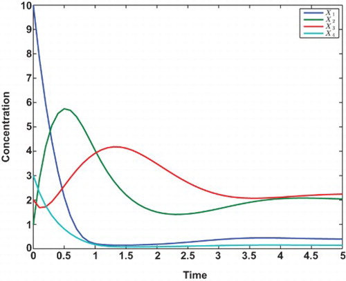
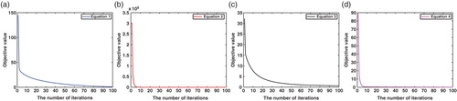
Figure 2. Objective values over various numbers of iterations in Algorithm 1.

3.1.2 Five-dimensional model

A benchmark five-dimensional model (Vilela et al., 2008; Yang, Dent, & Nardini, 2012) is considered,

The data used in this example are generated with the initial condition , the same as in Yang et al. (2012). Figure 3 shows the time series data that are sampled in the interval [0, 0.5] with . Note that the states of all variables quickly converge to the steady state. Hence, only limited information on the dynamics of the system is contained in the data. We run Algorithm 1 for 100 times with different initial values obtained from Equation (26) with s=80% and select the one with minimum objective value as the solution. The results in Table 2 show the effectiveness of this algorithm: estimated values of parameters are close to the true values and the optimal objective values are all very small.

Figure 3. Time series data of the five-dimensional model.

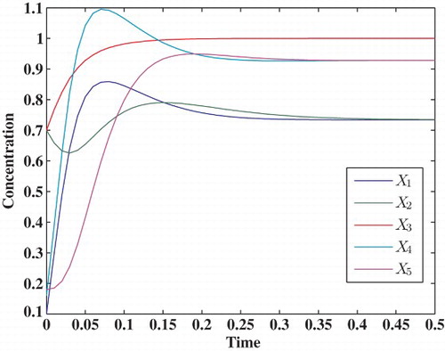
Table 2.  Estimated results of the five-dimensional model from Algorithm 1.

	True		Relative	Objective
Parameter	value	Estimation	error (%)	value
α1	5	4.7238	5.52
β1	10	9.7188	2.81
g13	1	1.1732	17.32
g15	−1	−1.0500	4.99
h11	2	2.0783	3.92
α2	10	10.0280	0.28
β2	10	9.9796	0.20
g21	2	1.9953	0.24
h22	2	1.9778	1.11
α3	10	9.0097	9.90
β3	10	9.0220	9.78
g32	−1	−1.1133	11.33
h32	−1	−1.1082	10.82
h33	2	2.1220	6.10
α4	8	7.5761	5.30
β4	10	9.5605	4.40
g43	2	2.1641	8.21
g45	−1	−1.0457	4.57
h44	2	2.0790	3.95
α5	10	9.9333	0.67
β5	10	9.9402	0.60
g54	2	2.0138	0.69
h55	2	2.0240	1.20

3.1.3 Six-dimensional model

In this example, Algorithm 1 is applied to estimate the parameters in the following six-dimensional S-system Yanget al. (2012):

The noise-free time series data are generated with the initial condition which matches that in Yang et al. (2012). Figure 4 illustrates the time series data which are sampled in the interval [0, 10] with Δ t=0.1. Figure 4 also shows the periodic oscillating behaviour of the data. The initial values are also chosen by Equation (26) with s=50%. The solution shown in Table 3 is the best one among 100 runs of Algorithm 1 with different initial values. The results in Table 3 indicate that the estimated parameters are close to their true values and the optimal objective values are all very small.

Figure 4. Time series data of the six-dimensional model.

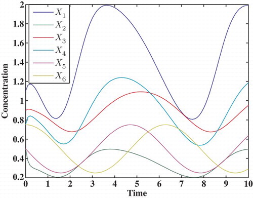
Table 3.  Estimated results of the six-dimensional model from Algorithm 1.

	True		Relative	Objective
Parameter	value	Estimation	error (%)	value
α1	10	9.7145	2.85
β1	5	4.8192	3.61
g13	−2	−2.0397	1.99
g15	1	1.0146	1.46
h11	0.5	0.5047	0.94
α2	5	4.7858	4.28
β2	10	9.9353	0.65
g21	0.5	0.5266	5.32
h22	0.5	0.5269	5.39
α3	2	2.0059	0.29
β3	1.25	1.2580	0.64
g32	0.5	0.4963	0.74
h33	0.5	0.4964	0.72
α4	8	8.0231	0.29
β4	5	5.0138	0.28
g42	0.5	0.5002	0.04
h44	0.5	0.5002	0.05
α5	0.5	0.4962	0.76
β5	1	0.9978	0.22
h56	1	1.0086	0.86
α6	1	0.9978	0.22
β6	0.5	0.4962	0.76
g65	1	1.0087	0.87

3.2 Performances of Algorithm 2

The performances of Algorithm 2 is studied in this example. We apply the algorithm to the data generated from the four-dimensional, five-dimensional, and six-dimensional models, respectively. The time series data we use are exactly the same as above-mentioned examples. Since Algorithm 2 solves the problem (10) which includes a range constraint for each parameter, the initial values for the algorithm are randomly generated in those ranges. In this study, the rate constants are restricted in the range [0.1, 10] and kinetic orders are in the range [−2, 3]. For each model, we run the algorithm for 100 times with different initial values and choose the one with minimum objective value as the final result. The estimated results from Algorithm 2 for each model are reported in the Tables 4–6. From the results, it can be seen that estimated parameters for the four-dimensional and six-dimensional models have very small relative errors compared with their corresponding true values. For the five-dimensional model, most parameters are estimated with low errors, while the estimations of the parameters in the third ODE have relatively large errors. This may be due to the limited information contained in the time series data. We can also see that the estimated objective function values for these three models are all very small. All these results show the effectiveness of the proposed algorithm.

Table 4.  Estimated results of the four-dimensional model from Algorithm 2.

	True		Relative	Objective
Parameter	value	Estimation	error (%)	value
α1	12	11.945	0.4585
β1	10	9.9288	0.7119
g13	−0.8	−0.807	0.8789%
h11	0.5	0.5034	0.6858
α2	8	7.9857	0.1787
β2	3	2.9912	0.2931
g21	0.5	0.5005	0.1093
h22	0.75	0.7511	0.1411
α3	3	3.0337	1.1233
β3	5	5.0244	0.4879
g32	0.75	0.7435	0.8691
h33	0.5	0.4937	1.26
h34	0.2	0.1964	1.7893
α4	2	2.0051	0.2528
β4	6	5.9847	0.2551
g41	0.5	0.4927	1.457
h44	0.8	0.7938	0.7776

Table 5.  Estimated results of the five-dimensional model from Algorithm 2.

	True		Relative	Objective
Parameter	value	Estimation	error (%)	value
α1	5	4.7704	4.5918
β1	10	9.7686	2.3138
g13	1	1.1535	15.3495
g15	−1	−1.0424	4.2402
h11	2	2.0652	3.2612
α2	10	10.0133	0.1333
β2	10	9.9644	0.3563
g21	2	2.0022	0.1122
h22	2	1.9845	0.7763
α3	10	8.1857	18.1435
β3	10	8.1839	18.1609
g32	−1	−1.2361	23.6145
h32	−1	−1.2363	23.6264
h33	2	2.2322	11.6124
α4	8	7.5565	5.5442
β4	10	9.5398	4.6023
g43	2	2.1688	8.4413
g45	−1	−1.0476	4.7607
h44	2	2.0827	4.1342
α5	10	9.9649	0.3505
β5	10	9.958	0.4204
g54	2	2.0152	0.7598
h55	2	2.0047	0.2345

Table 6.  Estimated results of the six-dimensional model from Algorithm 2.

	True		Relative	Objective
Parameter	value	Estimation	error (%)	value
α1	10	9.7512	2.4881
β1	5	4.9344	1.3118
g13	−2	−1.9891	0.5461
g15	1	0.9872	1.2845
h11	0.5	0.4899	2.0172
α2	5	4.6623	6.7549
β2	10	9.6115	3.8853
g21	0.5	0.5221	4.4167
h22	0.5	0.5218	4.3684
α3	2	1.9983	0.084
β3	1.25	1.2484	0.1248
g32	0.5	0.5005	0.0925
h33	0.5	0.5005	0.0912
α4	8	7.9848	0.1896
β4	5	4.9926	0.1487
g42	0.5	0.4996	0.0864
h44	0.5	0.4995	0.0953
α5	0.5	0.4991	0.1864
β5	1	0.9994	0.0609
h56	1	1.002	0.1989
α6	1	0.9977	0.2326
β6	0.5	0.496	0.8035
g65	1	1.0091	0.9094

4. Conclusions

The S-system is an effective mathematical model to characterize and analyse the molecular biological systems. The parameters in S-systems have significant biological meanings. However, the estimation of these parameters from time series biological data is non-trivial, because of the nonlinearity and complexity of this model. An novel method, the AFGCD, is proposed in this study to estimate the parameters of S-systems. To solve the nonlinear optimization problem involved in the parameter estimation, the proposed method optimizes one parameter at a time. Taking advantage of a property of the exponential function, an auxiliary function is constructed for each kinetic order parameter. We prove that updating the parameter value by optimizing the auxiliary function keeps the objective function nonincreasing. As the auxiliary function is quadratic, the analytical solution exists and therefore the updating rule for each parameter is simple and efficient. Based on this idea, two algorithms are developed: one estimates the parameters in S-system with the only non-negative constraints on rate constants; the other puts constraints both on rate constants and kinetic orders. Their performances are studied in simulation examples, which show that the estimated parameter values from the proposed algorithms are very close to the corresponding true values and the optimized objective functions has very low values. All of these results demonstrate the effectivenesses of the proposed algorithms.

In this study, the topology information of the system is assumed to be known. One direction of the future work is to extend the current method with structure identification method to infer the S-system without knowing the system topology.

This study is supported by Natural Science and Engineering Research Council of Canada (NSERC).

REFERENCES

- Bazaraa, M. S., Sherali, H. D., & Shetty, C. M. (2006). Nonlinear programming: Theory and algorithms. Hoboken, NJ: Wiley-Interscience. ISBN 0471486000.
- Beck, J. V., & Arnold, K. J. (1977). Parameter estimation in engineering and science. New York: Wiley.
- Bertsekas, D. P. (1999). Nonlinear programming. Belmont, MA: Athena Scientific. ISBN 1886529000.
- Chou, I.-C., Martens, H., & Voit, E. (2006). Parameter estimation in biochemical systems models with alternating regression. Theoretical Biology and Medical Modelling, 3(1), 25. ISSN 1742-4682. doi: 10.1186/1742-4682-3-25
- Gardner, T. S., di Bernardo, D., Lorenz, D., & Collins, J. J. (2003). Inferring genetic networks and identifying compound mode of action via expression profiling. Science, 301(5629), 102–105. doi: 10.1126/science.1081900
- Gonzalez, O. R., Kper, C., Jung, K., Naval, P. C., & Mendoza, E. (2007). Parameter estimation using simulated annealing for S-system models of biochemical networks. Bioinformatics, 23(4), 480–486. doi: 10.1093/bioinformatics/btl522
- Ho, S.-Y., Hsieh, C.-H., Yu, F.-C., & Huang, H.-L. (2007). An intelligent two-stage evolutionary algorithm for dynamic pathway identification from gene expression profiles. Computational Biology and Bioinformatics, IEEE/ACM Transactions on, 4(4), 648–704. ISSN 1545-5963. doi: 10.1109/tcbb.2007.1051
- Kikuchi, S., Tominaga, D., Arita, M., Takahashi, K., & Tomita, M. (2003). Dynamic modeling of genetic networks using genetic algorithm and S-system. Bioinformatics, 19(5), 643–650. doi: 10.1093/bioinformatics/btg027
- Klipp, E., Herwig, R., Kowald, A., Wierling, C., & Lehrach, H. (2005, May). Systems biology in practice: Concepts, implementation and application. Weinheim: Wiley-VCH.
- Li, L.-X., Wu, L., Zhang, H.-S., & Wu, F.-X. (2013). A fast algorithm for nonnegative matrix factorization and its convergence. Neural Networks and Learning Systems, IEEE Transactions, PP(99), 1. doi: 10.1109/TNNLS.2013.2280906
- Liu, L.-Z., Wu, F.-X., & Zhang, W.-J. (2012a). Alternating weighted least squares parameter estimation for biological s-systems. 2012 IEEE 6th international conference on systems biology (ISB), Xi'an, China, pp. 6–11. doi: 10.1109/ISB.2012.6314104
- Liu, L.-Z., Wu, F.-X., & Zhang, W. J. (2012b). Inference of biological s-system using the separable estimation method and the genetic algorithm. IEEE/ACM Transactions on Computational Biology and Bioinformatics, 9(4), 955–965. ISSN 1545-5963. doi: 10.1109/TCBB.2011.126
- Seung, D., & Lee, L. (2001). Algorithms for non-negative matrix factorization. Advances in Neural Information Processing Systems, 13, 556–562.
- Vilela, M., Chou, I.-C., Vinga, S., Vasconcelos, A., Voit, E., & Almeida, J. (2008). Parameter optimization in S-system models. BMC Systems Biology, 2(1), 35. ISSN 1752-0509. doi: 10.1186/1752-0509-2-35
- Voit, E. O. (2000, September). Computational analysis of biochemical systems: A practical guide for biochemists and molecular biologists. Cambridge, UK: Cambridge University Press. ISBN 0521785790.
- Voit, E. O., & Almeida, J. (2004). Decoupling dynamical systems for pathway identification from metabolic profiles. Bioinformatics, 20(11), 1670–1681. doi: 10.1093/bioinformatics/bth140
- Wang, H., Qian, L., & Dougherty, E. (2010, March). Inference of gene regulatory networks using S-system: A unified approach. Systems Biology, IET, 4(2), 145–156. ISSN 1751-8849. doi: 10.1049/iet-syb.2008.0175
- Wu, F.-X., & Mu, L. (2009, June). Separable parameter estimation method for nonlinear biological systems. ICBBE 2009. 3rd international conference on bioinformatics and biomedical engineering, Beijing, China, 2009, pp. 1–4. doi: 10.1109/ICBBE.2009.5163379
- Yang, X., Dent, J. E., & Nardini, C. (2012). An S-system parameter estimation method (SPEM) for biological networks. Journal of Computational Biology, 19(2), 175–187. doi: 10.1089/cmb.2011.0269