Actuator and sensor fault detection and isolation of an actuated seat via nonlinear multi-observers

Abstract

In this paper, a model-based approach to detect and to isolate sensors and actuators faults using nonlinear sliding mode observers is proposed for an actuated seat. The goal is to ensure the comfort and the security of the users in simulators applications. The principle is to reconstruct the state vector of the system by sliding mode observers and to compare the estimated outputs with those measured as residuals. In this work, a multi-observers technique is used. It consists of designing multiple observers such that each observer must be robust to noises and to other uncertainties but sensitive to each actuator or sensor fault. Simulation results are given to show the effectiveness of the approach.

Keywords:

• actuated seat
• dynamical modelling
• nonlinear sliding mode observers
• fault detection and isolation

1. Introduction

Nowadays, multimedia space simulators (flight simulator, automotive, video games, etc.) overgrown the field of new technologies. Users spend several hours a day on their chairs in front of the screens. For simulators, the user is in general installed on an articulated mobile platform equipped with an instrumented seat, a joystick and one or more widescreen. For example, to be efficient a racing simulator, the user have to feel every sensation as in real situation, such as, acceleration, brake or jumps.

In this study, which is part of an industrial project,¹we are interested in the diagnostic of the seat for such applications. Indeed, the seat is instrumented in a confined space and our objective is to ensure the comfort of the security of the users. Such systems integrate actuators, sensors and embedded intelligent systems (control, optimization, supervision, etc.) whose aim is to increase their performances. This context is motivating the present diagnostic study with application to an actuated seat which can be view as a robot with tree structure. Due to high reliability demands of such systems, recent supervision and fault diagnosis concepts are of particular importance (Isermann,1984, 2011; Patton, Frank, & Clarke, 1989; Sangha, Yu, &Gomm, 2013). Advanced methods of supervision and fault diagnosis need to satisfy the following requirements:

• Early detection of small faults with abrupt or incipient time behaviour.

• Diagnosis of faults in the actuators, process components or sensors.

• Detection of faults in closed loops.

• Supervision of processes in transient states.

Online diagnosis systems should not be considered without fault detection and isolation (FDI) module since undetected faults causing false alarms, missing detection and wrong diagnosis, generate at least distrust in the diagnosis system or even expensive damages. In closed-loop systems for the automatic control of robots, especially when the robot interacts with a human (Seddiki, Guelton,& Zaytoon, 2010), an erroneous feedback due to actuator fault may produce damages whose extent depends on the control system sensitivity to the incorrect measurement. In this case, sudden fault detection and its location are strongly recommended. The objective of an FDI is to determine if a fault is present in a system (fault detection), as well as to determine the kind, the location (fault isolation), the size, and the time-varying behaviour (fault identification) of the fault. The main purposes of this paper concern FDI of actuators around the actuated seat (robot with tree structure). Sensors offer important information and actuators deliver necessary inputs that allow the robot to automatically perform the tasks. FDI methods can be classified, according to the nature of the information on the reference behaviour, into mathematical model-based approaches and methods using information from historical data (Ding, Zhang, Naik, Ding, & Huang,2009; Godwin, Matthews, & Watson, 2013; Gorinevsky &Nicholas, 2013; Li, Yan, Yuan, Zhao, & Peng, 2011). In this context, our works are concerned with a mathematical model-based approach using the nonlinear sliding mode observer.

In the last few decades, most of works in the case of nonlinear systems are related to the concept of nonlinear observers (Hammouri, Kinnaert, & El Yaagoubi,1999; RÃos, Edwards, Davila, & Fridman, 2012) and sliding mode observers (Edwards, Spurgeon, & Patton, 2000; Slotine, Hedrick, & Misawa, 1986). To perform its tasks, the robot requires the implementation of a number of sensors and actuators intended to inform it about his environment and to deliver him necessary inputs, respectively. This is why it is important to detect and to locate each actuators and sensors faults as soon as possible in order to reconfigure the control law. Sliding mode observer methods are used in the literature for estimation and control (Davila, Fridman, &Poznyak, 2006; Levant, 1993; Nehaoua et al., 2013) and some works dealt with faults detection and reconfiguration (Bouibed, Seddiki, Guelton, & Akdag, 2013; Tan &Edwards, 2002; Yan & Edwards, 2007). A multi-observers technique is used in this work for actuators and sensors faults detection and isolation (Bouibed, Aitouche, & Bayart,2010; Edwards et al., 2000). It consists of the design of a set of sliding mode observers where each observer is dedicated to detect one actuator or sensor fault. In this case, each observer must be insensitive to the failure occurred on the actuator or sensor for which it is dedicated. To do so, this observer must be designed without using the input (or output) issued from the actuator (or sensor) it is dedicated to.

The paper is organized as follows: after the introduction, model-based FDI methods are briefly presented in Section 2. Then, the description and the modelling of the seat are given in Section 3. The sliding mode observers used to detect actuators and sensors faults are described in Section 4 and finally, some simulations are provided in Section 5 in order to illustrate the results obtained with the proposed approach.

2. Model-based FDI methods

The goal of this section is to present the basics of FDI which is often based on residuals generation. Several most frequently used residual-generation methods are:

• Parity space approach(Gertler, 1998): Parity equations are rearranged and usually transformed variants of the input/output or state/space models of the plant. The essence is to check the parity (consistency) of the plant models with sensor outputs (measurements) and known process inputs. Under ideal steady-state operating conditions, the so-called residual or the value of the parity equations is zero. In real situations, the residuals are non zero due to measurement and process noise, model inaccuracies, gross errors in sensors and actuators, and faults in the plant. The idea of this approach is to rearrange the model structure so as to get the best faults isolation. An application of this approach to sensors and actuators faults detection in the nonlinear case has been proposed recently in some of our preliminary studies (Bouibed, Aitouche,& Bayart, 2009).

• Parameters identification (estimation) approach: Diagnosis of parameter drifts which are not measurable directly requires online parameter estimation methods. Accurate parametric models of the process are needed, usually in the continuous domain in the form of ordinary and partial differential equations. Isermann (1984) surveyed different parameter estimation techniques such as least squares, instrumental variables and estimation via discrete-time models. These methods require the availability of accurate dynamic models of the process and are computationally very intensive for large processes. One of the most important issue in the use of parameter estimation approach for faults diagnosis is the complexity. The process model used could be either based on input–output data, nonlinear first principles model or a reduced order model.

• Observer-based approaches(Bouibed et al., 2010; Yang, Guo, Xing, Li, & Qiu, 2012): The main concern of observer-based FDI is the generation of a set of residuals which detect and uniquely identify different faults. These residuals should be robust in the sense that the decisions are not corrupted by such unknown inputs as unstructured uncertainties like process and measurement noise and modelling uncertainties. The method develops a set of observers, each one of which is sensitive to a subset of faults while insensitive to the remaining faults and the unknown inputs. The extra degrees of freedom resulting from measurement and model redundancy make it possible to build such observers. The basic idea is that in a fault-free case, the observers track the process closely and the residuals from the unknown inputs will be small. If a fault occurs, all observers which are made insensitive to the fault still have small residuals that only reflect the unknown inputs. On the other hand, observers which are sensitive to the fault will deviate from the process significantly and result in residuals of large magnitude. The set of observers is so designed that the residuals from these observers result in distinct residual pattern for each fault, which makes the fault isolation possible. Unique fault signature is guaranteed by design where the observers show complete fault decoupling and invariance to unknown disturbances while being independent of the fault modes and nature of disturbances.

In the sequel, our study will be focussed on observer-based approach. For this method, a model representing the seat is necessary and will be given in the following section.

3. Dynamical modelling of the actuated seat

In the following, we are interested in the design of the FDI method based on observers for an actuated seat which can be regarded as a robot with tree structure. This method uses the mathematical model of the system. That is why a dynamical model representing the seat is required. The model of the seat has the general form of second-order mechanical systems given as

where is a vector of generalized coordinates, J(q) is the inertia matrix, is the matrix of Coriolis and centrifugal forces, G(q) is the term of gravitational forces, is an uncertainty term related to the external disturbances and Γ is the vector of generalized forces produced by the actuators. The control input Γ is assumed to be given by some known feedback controllers. Note that J(q) is positive defined and so invertible.

The different matrices of the model are given as follows: where with These matrices are functions of the state variables and model parameters: Mis the total mass of the seat; m₄and m₆are, respectively, the masses of the footrest and the headrest of the seat; l₆is the distance between the axis of the joint θ₅and the centre of gravity of the headrest; L₃and L₆are, respectively, the lengths of the footrest and the headrest of the seat; β is the angle between the seat tracking axis and the soil; gis the gravitational acceleration; h₀, C₅, P₂₃and P₂₅are constants and functions of model parameters described above.

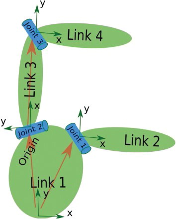
The dynamic model (1) is obtained by using Lagrangian formulations and Denavit–Hartenberg conventions for robots with complex chains (tree structure) (Khalil &Dombre, 2004). Figure 1shows an example of a tree structure with different joints and links.

Fig. 1. Open chain with tree structure.

The following observer-based approach is based on a state space representation. Therefore, to write the model in the state form we must express the acceleration q¨as a function of the other variables. So from Equation (1) one obtains the following expression:

Introducing the state variables x₁=q, and the control input u=Γ, the model (1) can be rewritten as the following state space model:

where , , g=J⁻¹and is the input vector.

The considered system is an actuated seat, depicted in Figure 2, which can be considered as a robot with tree structure. It contains five actuated joints and one unactuated joint θ₂whose significations are given in Table 1, where r_i(i=1, 4, 6) are prismatic joints and are rotary joints.

Fig. 2. Different joints of the seat.

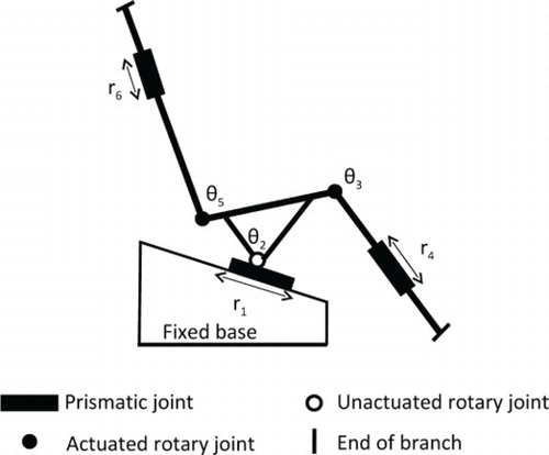
Table 1.  Joints significations.

r1	Tracking position expressed in m
θ2	Angle of the seating expressed in rad
θ3	Angle of the legrest expressed in rad
r4	Footrest position expressed in m
θ5	Angle of the seat-back expressed in rad
r6	Headrest position expressed in m

The signification of different joints of the seat is given in Table 1. For this system the state vector is constituted by the positions and the velocities of the actuated joints, i.e where is the vector of actuated joints positions and is the vector of actuated joints velocities.

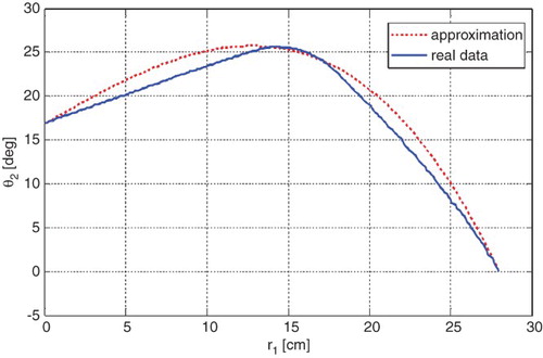
Note that θ₂is an unactuated joint (mechanical constraint) which is a function of the actuated joint r₁. This function can be approximated by a cubic polynomial such that: This approximation has been obtained through experimental data from kinematical measurements during a real movement of the seat.

Figure 3shows the approximation curve compared with the curve obtained by the experimental data acquisition.

The goal is now to design some observers dedicated to the diagnosis of the seat actuators and sensors faults.

Fig. 3. The approximation of θ₂with cubic polynomial.

4. Sliding mode observers design

The sliding mode observers used to estimate the states are described as follows (Bouibed, Aitouche, Rabhi, &Bayart, 2008; Davila, Fridman, & Levant, 2005; M'sirdi,Rabhi, Fridman, Davila, & Delanne, 2006; M'sirdi, Rabhi,Ouladsine, & Fridman, 2006):

where λ and α are diagonal observers gains matrices, diag(x) is a diagonal matrix whose diagonal entries are constituted by the elements of the vector x, xˆ₁and ◯₂are the estimates of x₁and x₂, respectively.

Let us consider and , the estimation errors. Their dynamics are given by

where .

Suppose that the states of the system (3) are bounded and take Δ f_jthe jth component of Δ f, so it exists for each component a positive constant , such that:

j=1, 2, … , 5.

In some cases, can be found by physical considerations (for example, the maximum acceleration of a motor is known). The convergence conditions of the observer (5) are given by the following lemma.

Lemma(Davila et al., 2005) Suppose that the condition (7) is satisfied for the system (3) and the parameters of the observer (5) are chosen such that:

where p_jare constants chosen such that 0<p_j<1. So, the observer (5) ensure the convergence of the estimated states to the real states (x₁, x₂) after a transitory phase and it exists an instant t₀such that for all t≥t₀, ,x₂).

Proof In order to prove the convergence of the state estimates to the real states, it is necessary to prove first the convergence of x˜₁and to zero. Assume that Equation (7) holds all the time. From Equations (6) and (7), estimation errors x˜₁and x˜₂satisfy the differential inclusion:

Differential inclusions are understood in the Filippov sense (Davila et al., 2005), so the second formula of Equation (9) turns into with x˜₁=0. The derivative of with obtain:

The trivial identity where η stands for each component of the vector x, is used here. In that case, when x˜₁>0 and , the trajectory is confined between the axis x˜₁=0, and the trajectory of the equation (Figure 4). Let be the intersection of this curve with the axis . Obviously, . It is easy to see that for x˜₁>0, :

Conditions (8) implies that

Inequality (12) ensures the convergence of the state to . Consider the dynamics of x˜₂to prove the finite time convergence. Obviously, at the moments when x˜₁=0 and taking into account that: obtain that holds in a small vicinity of the origin. Thus, where t_iare the time intervals between the successive intersections of the trajectory with the axis x˜₁=0. Hence, and the total convergence time is estimated by Therefore, Tis finite and the estimated states converge to the real states in finite time.

Fig. 4. Majorant curve for the finite time convergent observer.

For more details on this proof see Davila et al. (2005).

In the sequel, we are interested in actuator and sensor fault detection for the considered seat. To do this, two multi-observers schemes are employed, respectively, for actuators then sensors as described in the following paragraph.

4.1 Actuators faults detection and isolation

To detect actuators faults, a set of observers is used such that each observer is dedicated to detect one actuator fault. So the ith observer will have as inputs yand which is the vector of inputs without the ith input u_i. This structure is presented in Figure 5for the actuator FDI. In the considered seat, a set of five observers for each actuator is sufficient. Each observer generates one residual which is sensitive to only one actuator fault. This leads to the diagonal signature table to isolate actuator faults as presented in Table 2.

Fig. 5. Multi-observers for actuators faults detection and isolation.

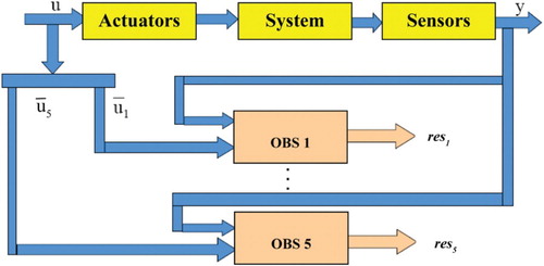
Table 2.  Actuators faults signature table.

	res1	res2	res3	res4	res5
	1	0	0	0	0
	0	1	0	0	0
	0	0	1	0	0
	0	0	0	1	0
	0	0	0	0	1

The ith observer dedicated to the ith actuator has the following structure:

4.2 Sensors faults detection and isolation

To detect sensor fault f_si, we generate a residual which is the estimation error given by the observer, r_i=e_yi. To isolate this fault occurred on sensor i, a state estimation must be done without using the output y_igiven by this sensor, so that the observer will not be robust to this fault. Thus, for msensors, must be designed at least mobservers.

For the actuated seat, we will therefore develop a bank of five observers so that they can detect and isolate failures in each sensor (five sensors). Figure 6shows the block diagram summarizing the method of detection and isolation of sensors faults using multi-observers. Each observer is dedicated to one sensor fault, consequently the generated residual will be sensitive to only this sensor fault. This leads to the diagonal signature table to isolate sensors faults as presented in Table 3.

Fig. 6. Multi-observers for sensors faults detection and isolation.

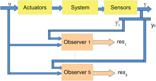
Table 3.  Sensors faults signature table.

	res1	res2	res3	res4	res5
sensor1	1	0	0	0	0
sensor2	0	1	0	0	0
sensor3	0	0	1	0	0
sensor4	0	0	0	1	0
sensor5	0	0	0	0	1

The ith observer dedicated to the ith sensor has the following structure:

4.3 Decision-making

In real conditions, residuals are never zero because of noises and uncertainties. Consequentially, thresholds must be fixed so that if a residual exceeds these thresholds it means that a fault occurs. The selection of each threshold should be based on the expressions of the residuals. Proper settings of the thresholds requires an accurate knowledge of the uncertainties and measurement noises which influence the residuals. In the linear case, if the parameters of the model and the measurement noises are Gaussian, the residuals will be Gaussian too. Therefore the thresholds can be set between more or less than 2 times the standard deviation of the residuals. Another way could be to use adaptive thresholds for nonlinear systems and improve the reliability of the decision (Hashemi & Pisu, 2011; Zhang, 2011).

Simulations trials have been given in the absence of faults, thresholds can be set on the basis of the maximum absolute values of the residuals. If some faults occur, they will cause deviations from zero of some residuals much greater than the differences caused by uncertainties an measurement noises. Thresholds should be chosen correctly in view to reduce the false alarms and the non detections. In our case, one assumes that the uncertainties and the measurements noises have not a great influence on the residuals.

5. Simulation results

To show the effectiveness of the approach, some simulations of some actuators and sensors faults are computed using Matlab/Simulink. Moreover, the parameters of the dynamical model are given in Table 4.

Table 4.  Parameters of the model.

Parameter	Value	Unit
M	17	kg
m4	2	kg
m6	1	kg
L3	0.3	m
L6	0.2	m
l6	0.7	m
β	0.327	rad
h0	0.324
C5	1.57
g	9.81
P23	9.81
P25	23.053

For simulations purposes the external disturbances have been chosen as additive random noise.

5.1 Actuators faults simulation

First, an abrupt fault on the tracking actuator is simulated twice, at 4.25 and at 15 s. Figure 7shows that the first residual res₁is sensitive to this fault while the others four are not sensitive. This residual is obtained using the first observer which does not use the first input u₁. Figure 8shows that the second residual res₂is sensitive to the legrest actuator fault while the others are not sensitive to this fault. This abrupt fault is similar to that simulated for the tracking actuator. Residuals res₃, res₄and res₅are sensitive to the footrest, the seat-back and the headrest actuator faults, respectively. These are clearly shown in Figures 9–11respectively. The obtained simulation results allows us to say that with the use of five observers as it is shown in Figure 5we can effectively detect and isolate faults in the five actuators of the seat.

Fig. 7. Detection of the tracking actuator fault.

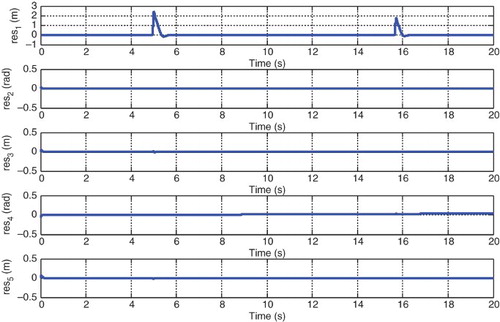
Fig. 8. Detection of the legrest actuator fault.

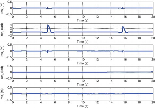
Fig. 9. Detection of the footrest actuator fault.

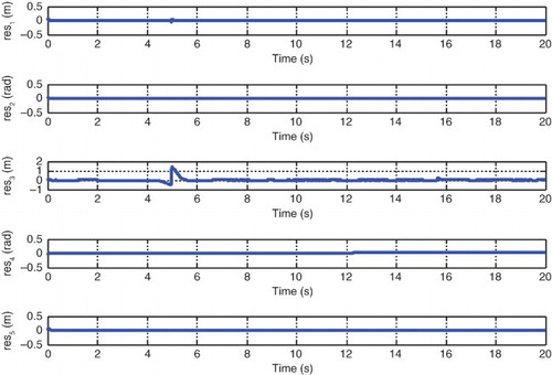
Fig. 10. Detection of the seat-back actuator fault.

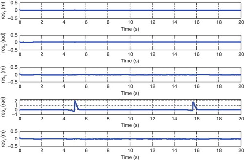
Fig. 11. Detection of the headrest actuator fault.

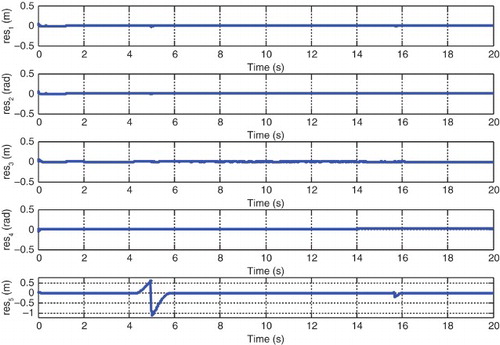
Thresholds are chosen as −0.5 for the minimum and +0.5 for the maximum within the simulations.

5.2 Sensors faults simulation

First, an additive fault on the legrest position sensor is simulated twice, at 4.25 and at 15 s. Figure 12shows that the second residual res₂is sensitive to this fault while the other residuals are not sensitive. This residual is obtained using the second observer which does not uses the second output y₂=x₂. Figure 13shows that the fourth residual res₄is sensitive to the seat-back position sensor fault while the others are not sensitive to this fault. The obtained simulation results allows us to say that with the use of five observers as it is shown in Figure 6we can effectively detect and isolate faults in the five sensors of the seat.

Fig. 12. Detection of the legrest position sensor fault.

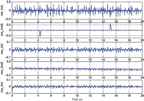
Fig. 13. Detection of the seat-back position sensor fault.

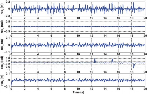
Thresholds are chosen as −0.2 for the minimum and +0.2 for the maximum within the simulations.

6. Conclusions

This work presents a nonlinear sliding mode observer-based FDI applied to a nonlinear model of an actuated seat. A multi-observers approach is used to generate residuals that allow us to detect and to isolate actuators and sensors faults. In the actuated seat, considered as a robot with tree structure, it is important to detect the faulty actuators or sensors and then to reconfigure the control law. The effectiveness of the approach allows avoiding false alarms and non detections. We notice that each residual is sensitive to only one actuator or sensor fault. These residuals are presented as fault signature matrix. Five observers are used for actuators faults and five for sensors faults. Each of them is dedicated to only one actuator or sensor. Therefore, 10 residuals are obtained and each of them is sensitive to only one actuator or sensor fault. Simulation results show that each residual generated by the sliding mode observers is sensitive to only one actuator or sensor fault. All real systems have uncertain characteristics, and cannot be modelled perfectly. Therefore, one has considered some bounded modelling uncertainties.

Notes

1. Confidentiality has been contracted with the industrial company, therefore, its name and the studied application cannot be provided in this paper. All the parts of this contract have read this paper and agreed to its publication.

REFERENCES

- Bouibed, K., Aitouche, A., & Bayart, M.(2009, August 9–12). Nonlinear parity space applied to an autonomous vehicle. IEEE international conference on mechatronics and automation, Changchun, China(pp. 198–203).
- Bouibed, K., Aitouche, A., & Bayart, M.(2010, June 23–25). Sensor and actuator fault detection and isolation using two model based approaches: Application to an autonomous electric vehicle. IEEE Mediterranean conference on control and automation, Marrakech, Morocco(pp. 1290–1295).
- Bouibed, K., Aitouche, A., Rabhi, A., & Bayart, M.(2008, June 30–July 2). Estimation of contact forces of a four-wheel steering electric vehicle by differential sliding mode observer. 1st IEEE Mediterranean conference on intelligent systems and automation, Annaba, Algeria (Vol. 1019, pp. 541–546).
- Bouibed, K., Seddiki, L., Guelton, K., & Akdag, H.(2013, October). Actuator fault detection by nonlinear sliding mode observers: Application to an actuated seat. 2nd international conference on control and fault tolerant control, Nice, France(pp. 739–743).
- Davila, J., Fridman, L., & Levant, A.(2005, November). Second-order sliding-mode observer for mechanical systems. IEEE Transactions on Automatic Control, 50(11), pp. 1785–1789. doi: 10.1109/TAC.2005.858636
- Davila, J., Fridman, L., & Poznyak, A.(2006, October). Observation and identification of mechanical systems via second order sliding modes. International Journal of Control, 79(10), 1251–1262. doi: 10.1080/00207170600801635
- Ding, S., Zhang, P., Naik, A., Ding, E., & Huang, B.(2009). Subspace method aided data-driven design of fault detection and isolation systems, Journal of Process Control, 19(9), 1496–1510. doi: 10.1016/j.jprocont.2009.07.005
- Edwards, C., Spurgeon, S. K., & Patton, R. J.(2000). Sliding mode observers for fault detection and isolation. Automatica, 36(4), 541–553. doi: 10.1016/S0005-1098(99)00177-6
- Gertler, J.(1998). Fault detection and diagnosis in engineering systems. Basel, NY: CRC.
- Godwin, J. L., Matthews, P., & Watson, C.(2013). Classification and detection of electrical control system faults through SCADA data analysis. Chemical Engineering Transactions, 33, 985–990.
- Gorinevsky, D., & Nicholas, M.(2013, October). Covariance estimation in two-level regression. 2nd international conference on control and fault tolerant control, Nice, France(pp. 288–293).
- Hammouri, H., Kinnaert, M., & El Yaagoubi, E. H.(1999). Observer-based approach to fault detection and isolation for nonlinear systems. IEEE Transactions on Automatic Control, 44(10), 1879–1884. doi: 10.1109/9.793728
- Hashemi, A., & Pisu, P.(2011). Adaptive threshold-Based fault detection and isolation for automotive electrical systems. 9th world congress on intelligent control and automation(pp. 1013–1018).
- Isermann, R.(1984). Process fault detection based on modeling and estimation methods – a survey. Automatica, 20(4), 387–404. doi: 10.1016/0005-1098(84)90098-0
- Isermann, R.(2011). Fault-diagnosis applications: Model-based condition monitoring: Actuators, drives, machinery, plants, sensors, and fault-tolerant systems. Berlin: Springer-Verlag.
- Khalil, W., & Dombre, E.(2004). Modeling, identification and control of robots. London: Kogan Page Ltd.
- Levant, A.(1993). Sliding order and sliding accuracy in sliding mode control. International Journal of Control, 58(6), 1247–1263. doi: 10.1080/00207179308923053
- Li, Z., Yan, X., Yuan, C., Zhao, J., & Peng, Z.(2011). Fault detection and diagnosis of a gearbox in marine propulsion systems using bispectrum analysis and artificial neural networks. Journal of Marine Science and Application, 10(1), 17–24. doi: 10.1007/s11804-011-1036-7
- M'sirdi, N., Rabhi, A., Fridman, L., Davila, J., & Delanne, Y.(2006, June). Second order sliding mode observer for estimation of velocities, wheel sleep, radius and stiffness. American control conference, Minneapolis, MN(pp. 3316–3321).
- M'sirdi, N., Rabhi, A., Ouladsine, M., & Fridman, L.(2006, June). First and high-order sliding mode observers to estimate the contact forces. International workshop on variable structure systems(pp. 274–279).
- Nehaoua, L., Ichalal, D., Arioui, H., Mammar, S., & Fridman, L.(2013). Lean and steering motorcycle dynamics reconstruction: An unknown input hosmo approach. American control conference, Washington, DC(pp. 7–15).
- Patton, R., Frank, P., & Clarke, R.(1989). Fault diagnosis in dynamic systems: Theory and application. Upper Saddle River, NJ: Prentice-Hall, Inc.
- RÃos, H., Edwards, C., Davila, J., & Fridman, L. M.(2012). Fault detection and isolation for nonlinear systems via HOSM multiple observer. Proceedings of the 8th IFAC symposium on fault detection, supervision and safety of technical processes, Mexico City, Mexico, (Vol. 8, pp. 534–539).
- Sangha, S., Yu, D., & Gomm, J.(2013). Sensor fault detection, isolation, accommodation and unknown fault detection in automotive engine using AI. International Journal of Engineering, Science and Technology, 4(3), 53–65.
- Seddiki, L., Guelton, K., & Zaytoon, J.(2010). Concept and Takagi-Sugeno descriptor tracking controller design of a closed muscular chain lower-limb rehabilitation device. IET Control Theory Applications, 4(8), 1407–1420. doi: 10.1049/iet-cta.2009.0269
- Slotine, J. J. E., Hedrick, J. K., & Misawa, E. A.(1986). Nonlinear state estimation using sliding observers. IEEE conference on decision and control, Athen, Greece(pp. 332–339).
- Tan, C. P., & Edwards, C.(2002). Sliding mode observers for detection and reconstruction of sensor faults. Automatica, 38(10), 1815–1821. doi: 10.1016/S0005-1098(02)00098-5
- Yan, X. G., & Edwards, C.(2007). Nonlinear robust fault reconstruction and estimation using a sliding mode observer. Automatica, 43(9), 1605–1614. doi: 10.1016/j.automatica.2007.02.008
- Yang, M. H., Guo, S. C., Xing, Z. R., Li, Y., & Qiu, J. Q.(2012). Actuator fault detection and isolation for robot manipulators with the adaptive observer. Advanced Materials Research, 482, 529–532.
- Zhang, X.(2011). Sensor bias fault detection and isolation in a class of nonlinear uncertain systems using adaptive estimation. IEEE Transactions on Automatic Control, 56(5), 1220–1226. doi: 10.1109/TAC.2011.2112471