A model predictive control framework for centralised management of a supply chain dynamical system

Abstract

In this paper, a centralised model predictive control (MPC) strategy is applied to control inventories in a four-echelon supply chain. The single MPC controller used in this strategy optimises globally and finds an optimal ordering policy for each node. The controller relies on a linear discrete-time state-space model to predict system outputs and the prediction can be approached by either of the two multi-step predictors depending on the measurability of the controller states. The objective function has a quadratic form and thus the resulting optimisation problem can be solved via standard quadratic programming. Simulation results show that a centralised MPC strategy is preferred because it can track customer demand and, in the meantime, maintain a proper inventory position level with reduced bullwhip effect.

Keywords:

• model predictive control
• supply chain
• bullwhip effect
• multi-step predictor

1. Introduction

Supply chain management (SCM), or supply chain optimisation, is a set of approaches utilised to efficiently integrate suppliers, manufacturers, distributors, and retailers, so that products are distributed at the right quantities, to the right locations, and at the right time, in order to minimise system-wide costs while satisfying service-level requirements (Aghezzaf, Sitompul, & Van Den Broecke, 2011). The last decades have witnessed a transition of the production of industrial goods from the local or national level to facilities with global outreach that serve international markets. This development has put substantial stress on the supply chain of today's enterprises. Viewed as a complex system, there are many aspects to study in supply chain management. One of these focuses on the improvement of inventory management policies, the goal of which is to maintain the inventory level at each echelon by ordering products from the upstream suppliers in order to satisfy the customers’ demands. The downstream flow rates of the products within the supply chain network depend on the customer demands, the upstream flow of information (orders), and the policies that every echelon uses to place orders and to replenish its inventories. The type of inventory policy has a significant effect on the variability of order quantities and inventory levels at various echelons of a supply chain. An important phenomenon in SCM first observed by Forrester (1961) suggests that the order variability increases along the upstream direction in the supply chain. Subsequently this observation is coined by Lee, Padmanabhan, and Whang(1997a, 1997b) as the bullwhip effect. It is a well-known phenomenon in supply chains’ operations. In a serial supply chain that consists of a factory, a distributor, a wholesaler, and a retailer, it can be observed that the retailer's orders to wholesaler display larger variability than the end-consumer's demand, the wholesaler's orders to its supplier show even more oscillation, and the factory's production plan is the most volatile. The common symptoms of such variations could be excessive or insufficient inventory holding, bad demand forecast, poor customer service level, and uncertain production planning (Lee et al., 1997a). The bullwhip effect has been recognised as one of the main obstacles to improve supply chain performances and thus tackling this problem has received increasing attention in the SCM literature.

The approach this paper advocates is to develop decision policies of SCM based on a control-oriented formulation in order to achieve bullwhip mitigation and optimal supply chain operations. Recent works utilising model predictive control (MPC) have been found to provide an attractive solution for SCM. MPC was first applied to inventory management by Kapsiotis and Tzafestas (1992) for a single manufacturing site problem. This development has subsequently led to an increasing number of reports on the application of MPC to SCM in the last decade. Perea-Lopez,Ydstie, and Grossmann (2003) employed an MPC scheme as an optimisation tool to manage a multi-echelon multi-product supply chain with deterministic demand, so the need for an inventory control mechanism was reduced. They showed that the centralised structure exhibited superior performances to the two decentralised approaches via simulation on a complex supply chain. Lin, Jang, andWong (2005) presented a minimum variance control system with two separate setpoints for the inventory level and the Work-in-Process (WIP) level. Their MPC control strategy outperformed the classical order-up-to (OUT) policy, proportional and integral control, and automatic pipeline variable inventory and order based production control system (APVIOBPCS) model control in maintaining inventory at desired levels while mitigating the bullwhip effect. Wang and Rivera (2008) examined the application of MPC to inventory control problems arising in semiconductor manufacturing. Maestre, Munoz de la Pena, andCamacho (2011) proposed a distributed MPC algorithm for a two-node supply chain. Each node minimised its local objective function over its own decision space as well as the decision space of the other node. The MPC algorithm takes a cooperative decision based on the multiple optimal objective function values (one for each node). Their method is not extendable to a supply chain with more than two nodes. Alessandri, Gaggero, and Tonelli (2011) combined min–max optimisation and MPC to solve inventory control problems for a multi-echelon, multi-product distribution centre. There are other MPC schemes developed for the specific supply chain network under study, which were different in the prediction models, optimisation algorithms, and implementation strategies they used. Mestan, Turkay,and Arkun (2006) used a hybrid system approach to model a multi-echelon supply chain, and they implemented a decentralised and non-cooperative MPC strategy to optimise a cost function that is related to the economic performance measures. Li and Marlin (2009) applied a robust MPC framework to a serial supply chain using an economic cost function. The latest development in the application of MPC to SCM is the distributed implementation. Subramanian,Rawlings, Maravelias, Flores-Cerrillo, and Megan (2013) proposed cooperative MPC scheme with closed-loop stability and used the method in a two-node supply chain as an example. A distributed MPC is presented by Ferramosca,Limona, Alvarado, and Camacho (2013) to track the changing non-zero setpoints and this strategy is applicable to any finite number of subsystems. The reader is referred to several proper review papers (Sarimveis, Patrinos, Tarantilis, & Kiranoudis, 2008; Subramanian et al., 2013) on the application of control engineering techniques to the SCM problems.

As can be seen from the literature (Braun, Rivera,Flores, Carlyle, & Kempf, 2003; Ferramosca et al., 2013; Li& Marlin, 2009; Wang & Rivera, 2008), there are several advantages of applying MPC to SCM. The MPC controller accomplishes the operational objectives such as tracking inventory targets and meeting customer demands. Moreover, MPC can minimise or maximise an objective function that represents a suitable measure for supply chain performance. MPC can be tuned to achieve stability and robustness in the presence of disturbance and stochastic demand as well as constraints on production, inventory levels, and shipping capacity (Wang & Rivera, 2008). Our previous work focused on a fully decentralised MPC strategy (Fu, Dutta, Ionescu, & De Keyser, 2012) to update ordering decisions for bullwhip reduction. Modern enterprises tend to expand their scales and interactions, thus it is not rare for them to own a whole supply chain. The primary motivations for developing such a centralised implementation of MPC are to highlight the role of the global coordinator of a supply chain and reduce the bullwhip effect. One often suggested scheme for reducing bullwhip effect is to centralise demand information, i.e. to make customer demand information available to every node of the supply chain. The purpose of this paper is to demonstrate the applicability of a fully centralised MPC to the problem of dynamic management of a benchmark supply chain network despite its feasibility for the supply chains where all nodes belong to one enterprise. With this implementation, ordering policy for each node of the supply chain is optimised by a global controller and the bullwhip is mitigated to a greater degree compared to our previous decentralised MPC ordering policy. Another benefit for this implementation is that it has flexibility to put different emphasises on reducing bullwhip for different echelons by assigning proper weights to control move suppression term of objective function.

The remainder of this paper is structured as follows. In Section 2, the four-node supply chain network is described and the discrete-time controller model for the overall supply chain system is developed. Using the centralised model, the two approaches to predictions on future system outputs are presented and a centralised MPC formulation is derived in Section 3. Simulation results in Section 4 show that an appropriate tuning of the parameters can be chosen to produce the required performances. Finally, some concluding remarks are given in Section 5.

2. Problem formulation

2.1 Supply chain system

In this section, one type of product and one node at each echelon are considered, but the method can address the case of multiple products and multiple nodes. Consider a serial supply chain model similar to the one used in Hoberg,Thonemann, and Bradley (2007) and Sundar andLakshminarayanan (2008). This supply chain network (depicted in Figure 1) consists of all the nodes involved in fulfilling a customer demand and there are four logistic echelons, a factory, a distributor, a wholesaler, and a retailer. Orders for products propagate upstream from right to left, and goods are shipped downstream in the opposite direction. In the general multi-product, multi-echelon supply chain, the operational decisions are made for each product individually and independently of other products. Consequently, emulating the supply chain model for one product at a time would still be valid but the methodology can be easily extended to larger networks at the expense of extra computational effort.

Figure 1. A four-node production–distribution supply chain system.

2.2 Notations and assumptions

• The decisions of ordering and shipment are made within equally spaced time periods, e.g. hours, days, or weeks. The duration and unit of base time period depend on the dynamic characteristics of the supply chain system.

• The set of supply chain node is denoted by . Each of the logistic echelons of the supply chain is denoted by i (i=1, 2, … , M). In this notation, (i+1) represents an immediate supplier and (i−1) an immediate customer of the ith node. Thereby, for this specific supply chain, i=1 represents the Retailer (Re) and i=4 represents the Factory (Fa).

• Any arbitrary node in Figure 1 is characterised by the following three variables. The inventory level Iⁱ(k) is the number of products at any discrete-time instant k in stock of node i. Due to the lead time delay L_i for shipment, inventory position is defined to better monitor the variations of inventory level and includes inventory plus products in transportation from its supplier. The ordering information is communicated instantaneously, but an order placed at time k can only be processed at time k+1 due to the sequence of events performed during supply chain operations. Therefore, standing order for each node is defined as the amount of order to be processed at time k+1. The available variables in the supply chain context will be reclassified in an MPC control sense. All the variables and their meanings in the supply chain setting are listed in Table 1.

• The sequence of events performed in the ith echelon is as follows. (1) At each discrete time k, the ith echelon receives a product; (2) the demand Oⁱ⁻¹(k) from the downstream node i−1 is observed and satisfied immediately, i.e. (if not backlogged because of insufficient inventory); (3) the new inventory level Iⁱ(k) is measured; and (4) the ith echelon places an order Oⁱ⁺¹(k)to the upstream node i+1.

• A time delay L_i is assumed for all shipment actions together with consideration of the nominal ordering delay such that products dispatched from node i+1 at time k will be available to node i at time k+L_i+1.

• The manufacturing process is modelled by a pure delay unit with the discrete transfer function being equal to z^−L, where L is the lead time.

• The end-customer demand follows an autoregressive moving average (ARMA) time series model of the form in the following equation:

  where z⁻¹ represents both of the backward shift operator and complex variable in z-transform. When applied to the time-dependent signal s(k), it becomes the backward shift operator, i.e. . The time series e(k) is a white noise with zero mean and unity variance. Polynomials of and Φ (z⁻¹) have proper orders depending on a certain demand pattern.

2.3 Dynamical model

To illustrate micro-dynamics of the supply chain network, consider any echelon , whose relationship with neighbouring echelons is shown in Figure 1. Its inventory position and in-hand inventory Iⁱ(k) satisfy a conservation law according to orders placed and received. Node i orders goods in the amount of Oⁱ⁺¹(k) from node i+1 at discrete times k=1, 2, … and receives the items after a constant lead time L_i. Note that, in this work the lead times are considered to be fixed over review periods and they can be obtained from the managers of the supply chain or estimated from gathered data. The conservation equations for the node's inventory position , in-stock inventory Iⁱ(k), and the standing order are

Table 1.  Variable mapping for the MPC controller.

Process variable	Supply chain information
Output	Inventory position IP ^i
Output	Standing order
Inputs	Amount of orders placed by node i to upstream node i+1, O^i+1
Inputs	Amount of products delivered to downstream node i−1 by node i, Y^i−1
Disturbance	Demand of downstream node i−1, O^i−1
Disturbance	Delivery from upstream node i+1, Y^i+1
Setpoint w^i	Inventory position target

Equations (2)–(4) define the system dynamics for the supply chain when complemented with the local ordering policies, i.e. the strategies for determining Oⁱ⁺¹(k) from available information at time k. The complete information set for the entire network includes the inventory records and Iⁱ(k) for all up to period k, and orders Oⁱ⁺¹ up to period k−1:

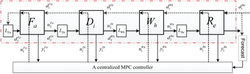
A fully centralised MPC strategy as shown in Figure 2 is proposed to be applied to the supply chain described above (in squared box). If all the facilities are owned by the same enterprise, the information is shared across the network, every node can determine its order quantities based on any subset of . Therefore, a centralised control scheme is appropriate and feasible. All available information is fed to the controller and the ordering decisions are determined by the global coordinator.

Figure 2. Centralised control scheme for supply chain operation.

Assume that the upstream suppliers always have ample goods in stock (Chen, Drezner, Ryan, & Simchi-Levi,2000; Lee, So, & Tang, 2000; Ouyang & Daganzo, 2006; Ouyang & Li, 2010) to meet their customers’ demands, then this approximation leads to the following two relations: and . Applying the two relations and taking the z-transform on both sides of the model (2) and using the process control variables result in

This discrete-time model for node i captures the basic dynamic features of material and information flow within the supply chain system. This relation frees n of 2n manipulated variables for the overall supply chain network with n nodes. Relations (2)–(5) will be used as the basic dynamical models in the design of the MPC control strategy. Combine the transfer function of each node into a whole system to derive the transfer function matrix: where is the end-customer demand. This model can be reorganised to give the overall model of supply chain in a state-space form (6) and (7) and will be used as the nominal controller model. The whole supply chain is modelled as a four-input/four-output system with the end-customer demand as a measured disturbance.

3. Centralised MPC strategy

MPC is a family of control strategies based on the explicit online use of a system model to calculate predictions of the future process output and to optimise future control actions over a period of time. MPC has gained wide acceptance in industries as the basis for advanced multivariable control schemes (Camacho & Bordons, 1999). In MPC, a system model is used to predict the future system outputs. The future control efforts are calculated by optimising a control-relevant objective function subject to some constraints on the inputs and outputs. The first control move is implemented and the calculations are repeated at the next sampling time using the new measurements and updated states. This is referred to as a rolling or receding horizon control strategy. There are several key elements characterising MPC formulation, which are summarised in the following section.

3.1 Controller model

The purpose of this section is to present the derivation of a fully centralised MPC strategy to further reduce order variability. In Figure 2, the supply chain network is controlled based on a centralised architecture, where the whole supply chain is treated as a single system and implemented by a monolithic MPC controller. The controller model provides a prediction of future supply chain network outputs as a function of manipulated variables and estimated disturbances. The controller model is part of the control system, and its states may be partially or fully known. In the present work, the controller model has the form of a general linear discrete-time state-space:

The input vector definition is , where the inputs u, d, w,and v represent manipulated variables, load disturbances, and two unmeasured disturbances, respectively. The matrices B and D in the controller model are partitioned by and D=[0, D_d, 0, D_v]. The dynamical models of all nodes could be reorganised to give the overall model of supply chain in a state-space form (6) and (7) and will be used as the nominal controller model. The manipulated input vector u physically corresponds to the orders placed by supply chain nodes, while measured disturbance d represents the forecasted customer demand. The output vector y consists of an inventory position at every node.

3.2 The multi-step predictors

The methods for predicting future outputs are approached by two ways depending on whether the system states can be directly observed. If the state variables of the controller model are measurable as in the case of our model, the multi-step predictor is developed from the state-space model according to Equation (8). The derivation of the predictor is given in Section 3.2.1. Otherwise, the predictor has to be obtained by state estimation when the states are not fully measurable. The result is given in Section 3.2.2.

3.2.1 Multi-step predictor based on measured states

At each time instant k, controller models (6) and (7) are used to predict future output , where and N₂ is the prediction horizon. When the system states can be fully observed, the MPC controller models (6) and (7) take the following linear discrete-time state-space form (Lee &Yu, 1994):

Since MPC needs prediction for future behaviour of output, not of all the states, it is convenient to lump the effect of manipulated variables, D_u=0, and express it directly through the system state instead of at output. One of the primary goals for using centralised MPC implementation is to reduce the bullwhip effect by alleviating the demand fluctuation along the upstream direction in the supply chain. The demand propagates within the chain in the form of orders placed at each echelon. The bullwhip reduction can be anticipated if the change on orders (manipulated variables u in differenced form Δ u) is penalised in the objective function (15). The following optimal multi-step prediction equation is preferred by iterating the difference form of models (8) and (9):

where is the output predictions vector over the prediction horizon N₂ based on measurement at time k; represents the vector of future control moves (control increments) over the control horizon N_u and we also allow the flexibility of suppressing the last N₂−N_u input moves a priori (i.e.. The vector of corresponds to the forecast of demand in a differenced form over the control horizon N_u. It explains how forecast of customer demand (measured disturbance) influences the predicted inventory position (output). In the SCM context, taking use of forecasted demand in the control algorithm is a significant contributor to improved performances. They relate to output through the following dynamic matrices:

Here Δ operator represents the change of the variable from its previous sampling time, i.e. . The state variable x(k) is directly measurable in this case so that Δ x(k) is available at time period k. Obviously Equation (10) contains two parts, one representing the contribution of the initial state Δ x(k) and output y(k) known at time k, and the second part is determined by the optimising future control efforts and predicted disturbances .

3.2.2 Multi-step predictor based on state estimation

It is often highly unrealistic to assume that all states of the system and disturbances are measurable. When the measurement of the state vector is unavailable, an estimator must be used. The predictions of future unmeasured disturbances are assumed to be zero and the nominal models (8) and (9) are used to estimate the future states of the system:

where is the estimate of the states at future time period k+1 based on the information available at time period is the estimate of the system outputs at time period k based on information at k−1, and is the innovation term of the estimator error is the system outputs) to account for unmeasured disturbances. K is a constant gain matrix and Lee and Yu (1994) recommended that it is set equal to Kalman filter gain.

The measurements of the system outputs y(k) and the measured disturbances d(k) have been obtained at the start of time period k, and the state estimate and estimator error can be calculated from Equations (11) and (12). The future control actions are optimised to be , where . The future values of load disturbances are structured wisely as forecasted demand by using forecasting methods and the disturbance vector is denoted by . For simplicity, are assumed to be

The multi-step prediction equation is developed by recursively using Equations (11) and (12) and considering the assumption (13):

where is the output prediction of the supply chain system based on the measurements until time period , and is a vector of optimising future control variables, , and the last three terms in Equation (14) are known at the start of time period k. The pulse response matrix S^u and the other matrices S^d, S^x, and S^e are given as follows:

The differenced form of the predictor based on state estimation is obtained by defining as with

Both approaches to the multi-step predictor are presented in these two sections. The two multi-step predictors can be chosen depending on the measurability of the state of the controller model.

3.3 Objective function

The predicted process outputs depend on not only the past inputs and outputs but also the future control scenario . The task of the MPC controller is to calculate the control vector by minimising a specified objective function of any form in general. In the application of the MPC framework to SCM, the controller considers at each time period k the previous information on inventory positions, actual customer demands, orders for all the nodes of the supply chain network as well as the future information on inventory position setpoints, and forecasted demands in order to calculate a sequence of future order decisions on the basis of the following objective function:

where is the inventory position reference vector for time k+j projected at time k, Q(j) and P(j) are penalty weights on control error and control move size, respectively, which enable the controller to satisfy inventory position setpoint tracking and adjust order variability. The small variation of demand at retailer end will be amplified along the upstream direction and this phenomenon is known as the bullwhip effect. The second term in Equation (15) penalises excess changes of ordering decisions, which is expected to reduce the bullwhip effect. In addition, suppression of excess movement of the orders is desired for the echelon of factory because this action leads to a smoothed order pattern and thus results in reduced variability on factory starts. The objective function can be described in a vector form:

where the reference vector is and the penalty matrices and are used to penalise the deviation of inventory positions from their targets and the control move size, respectively. Because the demands change in every time period, the setpoints for inventory positions need to be adapted and updated to an economic level in every time period so that customer's demands can be satisfied and inventory holding cost should be reduced. A first-order reference trajectory (De Keyser, 2003) is chosen and the setpoints are updated according to the decision rules proposed in Dejonckheere,Disney, Lambrecht, and Towill (2003). In addition to this control-oriented objective function, an economic cost function (Li & Marlin, 2009; Mestan et al., 2006) could be optimised in centralised or decentralised implementation.

3.4 Optimisation problem formulation

The control of supply chain is now formulated as an optimisation problem in which the control moves are computed on the basis of the objective function (16) subject to the linear inequality constraints. Some practical requirements in SCM operations may be appropriately posed as constraints on the system variables. Three types of constraints are considered in most of studies depending on practical conditions of the supply chain operations.

• Output variable constraints. The controller minimises the deviation of the inventory position of each node from their setpoints. But the inventory positions can only stay within high and low limits due to capacity constraints:

  To avoid infeasible solution to the optimisation problem, the constraints on system outputs are applied as soft constraints in Equation (16), which is in practice a commonly used technique to address this problem.

• Manipulated variable rate constraints. There are some hard low and high bounds for changes (or moves) on orders of each node. If proper constraints on changes of orders are applied, demand variation reduction can be expected within the supply chain and thus result in less fluctuation in factory thrash:

• Manipulated variable constraints. In addition to the constraints on change of order, there are some high limits on the ordering quantities on account of transportation capacity limitation:

The MPC control law requires not too much computation effort in the absence of constraints. In the presence of constraints (17)–(19), the MPC formulation based on the objective function (16) and prediction equation (10) or (14) is then solved by standard quadratic programming algorithms (Fletcher, 1981) subject to appropriate inequality constraints:

where the gradient vector and the Hessian matrix of the objective function are to be constructed according to different prediction equations, respectively. In centralised implementation, a single controller is used by a global coordinator to make ordering decisions for each node. The centralised MPC controller, based on overall models (6) and (7) of the supply chain network, calculates all the control moves via the optimisation problem (Equation (20)) and sends the first element of as ordering decisions at current time k to each echelon.

4. Illustrative example

4.1 Initialisation of the supply chain model

The supply chain is considered over 100 weeks (i.e. the base time is 1 week and the simulation is reviewed over 100 weeks). The market demands modelled in Equation (1) are generated according to the following equation:

where μ=8 is the mean for the ARMA demand pattern, and the autoregressive coefficient and the moving average coefficient are assumed to be ϕ=0.8 and θ=0.6, respectively. The forecasted demands are approached by ten-week moving average of actual demands and both of them are shown in Figure 3. The system models are initialised by setting parameters as in Table 2. It reports the supplier's production/transportation delay (PTD), initial inventory level (IIL), and initial Work in Process (iWIP) at each node. Handling efficiently the constraints for manipulated and/or controlled variables is indeed one of the important abilities of MPC. However, the constraints are not considered in conventional OUT and fractional ordering policies, and the performances of a centralised MPC strategy need to be compared with them under the same conditions in simulation. Therefore, no constraints on the inventory positions and orders are posed in the numerical simulation so that the supply chain can be operated under free conditions. The SCM problem can still benefit from the application of MPC in other aspects, e.g. keeping desired inventory, tracking customers’ demand, and reducing bullwhip effect.

Figure 3. Actual and forecasted customer demand.

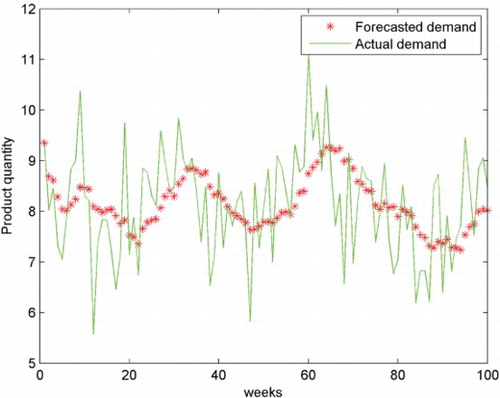
Table 2.  Simulation data and initial state of supply chain operation.

Supply	PTD	IIL (units	iWIP (units
chain node	(weeks)	of product)	of product)
Retailer	2	10	5
Wholesaler	2	10	5
Distributor	2	10	5
Factory	2	10	5

4.2 Tuning the centralised supply chain controller

One of the advantages for the MPC strategy is its flexibility to tune the controller parameters to meet the required performances. In this simulation example, the prediction horizon is N₂=15 and the control horizon is N_u=10, both of which exceed the collective sum of the one-week nominal ordering delay and two-week transportation time at each node over four serial nodes in the supply chain. The long horizons are demanded by the centralised decision-making in order to execute necessary feed-forward anticipations. The output weight matrix is set in a way that it is 1 for each controlled variable, while the move suppression matrix is tuned to compare effects of different weights on bullwhip effect reduction.

The time behaviours of the inventory positions and orders are shown in Figure 4 when no penalty is applied to the move sizes of orders. The ordering decisions are adjusted aggressively at first time periods and inventory positions keep a small fluctuation after the 40th week. The results in Figure 4 only show the control efforts and outputs for the first 50 weeks in order to scrutinise the initial system response in proper Y-axis scale. The weights on move sizes are set equal for each controlled variable in the next simulation experiment and the results are given in Figure 5. The variance magnitude of the orders is amplified from retailer to factory at first time periods as observed in Figure 5(a) but from Figure 5(b) it can be observed that the order decisions between weeks 50 and 100 keep a good tracking of end-customer demand variation. The oscillation on inventory position is mainly caused by tracking the setpoints. If the weight on move size of the factory order is increased and the other weights remain unchanged, then its ordering decision is smoothed and stabilised as shown in Figure 6. This smoothed ordering pattern is similar to the one generated by fractional ordering policy (Dejonckheere et al.,2003), and it is favourable because the factory thrash will not vary violently caused by its manufacturing orders from very large amount to very low amount or vice versa. But the downside is that the suppression on move sizes of orders increases the variability of inventory positions, which can be seen from weeks 50–100.

Figure 4. Control effort and output (IP) of the first 50 weeks when weights on move size P(j)=0.

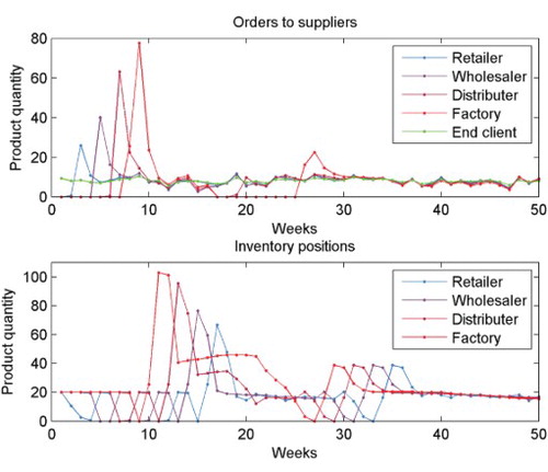
Figure 5. (a). Simulation results of the first 50 weeks with weights on move size of identity matrix P(j)=I. (b). Simulation results of 50th–100th weeks with weights on move size of identity matrix P(j)=I.

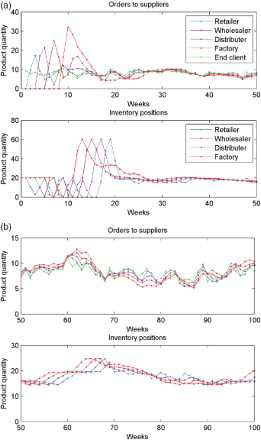
Figure 6. Control effort and output (IP) with move size of different weights P(j)=[1 0 0 0; 0 1 0 0; 0 0 1 0; 0 0 0 5].

Using the definition of bullwhip effect proposed by Disney and Towill (2003), the comparisons among numerical bullwhip quantities generated by different weights P(j) on move sizes and that caused by a decentralised MPC strategy ordering policy and conventional ordering policies (Fu et al., 2012) are presented in Table 3. The ratio of variance to mean of orders at each node is calculated based on simulation samples.

Table 3.  Ratio of variance to mean for ordering data of each node generated by conventional ordering policies, decentralised MPC ordering policy, and centralised MPC with different weights P(j) on control move and the bullwhip over the supply chain.

Ordering policies	Retailer	Wholesaler	Distributor	Factory	Bullwhip over supply chain
P(i)={0; 0; 0; 0}	0.9306	2.1218	5.2003	8.7939	9.4494
P(i)={1; 1; 1; 1}	0.4197	0.8424	1.3603	2.8501	6.7902
P(i)={1; 1; 1; 5}	1.9038	4.0456	4.4986	1.7157	0.9012
Decentralised MPC	0.1416	0.2647	0.4186	0.6020	4.2500
Fractional ordering	0.2059	0.5277	1.0061	1.3644	6.6258
Order-up-to policy	0.3803	0.6859	1.6506	3.2333	8.4905

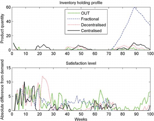
Table 3 shows that the ordering policies based on the MPC configurations outperform the conventional ordering policies in the sense of bullwhip reduction. These results demonstrate the flexibility through centralised MPC to put different emphases on bullwhip suppression for different nodes. When larger weight is put on changes of factory orders, it has a smoothed order pattern to reduce variance of factory thrash. There is a trade-off because if a desired order rate is used then large deviation of inventory positions from their targets is found. The profile of the customer satisfaction level is determined by comparing the absolute values of the difference between the product transferred out of the retailer echelon and the end-customer demands, which is shown in the lower part of Figure 7. The smaller the absolute values, the higher is the satisfaction level. The result shows that the well-tuned centralised MPC strategy has better customer satisfaction level than the other strategies and inventory holding profile is desired because it is made as close to zero as possible while being kept to a good customer satisfaction level.

Figure 7. Absolute difference between the transferred product and the demand as inverse of the customer satisfaction level and inventory holding profiles for four different control configurations.

5. Summary

MPC has long been a successful technique in process control applications. In this paper, a method for determining ordering policy is derived using the centralised MPC control scheme. The dynamic models are presented that consider the flows of product and information within the supply chain. Two approaches to predictions on system outputs are formulated and these two multi-step predictors rely on a linear discrete-time state-space model. The centralised MPC optimisation problem can be transformed to standard quadratic programming with the proposed formulation. A numerical example shows that MPC-based ordering polices can significantly lower the impact of demand variability in the supply chain compared to conventional ordering policies. Tuning parameters play an important role in achieving desired performances for supply chain operations. It has been illustrated in the simulation that this control strategy could be tuned for different performance requirements. Good results are observed because centralised MPC implementation has full knowledge of system models and information flows, which allows it to coordinate the decisions made by each node of the supply chain.

REFERENCES

- Aghezzaf, E.-H., Sitompul, C., & Van Den Broecke, F. (2011). A robust hierarchical production planning for a capacitated two-stage production system. Computers & Industrial Engineering, 60(2), 361–372. doi: 10.1016/j.cie.2010.12.005
- Alessandri, A., Gaggero, M., & Tonelli, F. (2011). Min-max and predictive control for the management of distribution in supply chains. IEEE Transactions on Control Systems Technology, 19, 1075–1089. doi: 10.1109/TCST.2010.2076283
- Braun, M. W., Rivera D. E., Flores, M. E., Carlyle, W. M., & Kempf, K. G. (2003). A model predictive control framework for robust management of multi-product, multi-echelon demand networks. Annual Reviews in Control, 27, 229–245. doi: 10.1016/j.arcontrol.2003.09.006
- Camacho, E. F., & Bordons, C. (1999). Model predictive control. London: Springer-Verlag.
- Chen, F., Drezner, Z., Ryan, J., & Simchi-Levi, D. (2000). Quantifying the bullwhip effect in a simple supply chain: The impact of forecasting, lead times, and information. Management Science, 46(3), 436–443. doi: 10.1287/mnsc.46.3.436.12069
- Dejonckheere, J., Disney, S. M., Lambrecht, M. R., & Towill, D. R. (2003). Measuring and avoiding the bullwhip effect: A control theoretic approach. European Journal of Operational Research, 147, 567–590. doi: 10.1016/S0377-2217(02)00369-7
- De Keyser, R. (2003). Model based predictive control. Invited Chapter in UNESCO Encyclopaedia of Life Support Systems (EoLSS). Article contribution 6.43.16.1. Oxford: Eolss Publishers Co. Ltd.
- Disney, S. M., & Towill, D.R. (2003). On the bullwhip and inventory variance produced by an ordering policy. The International Journal of Management Science, 31, 157–167.
- Ferramosca, A., Limona, D., Alvarado, I., & Camacho, E. F. (2013). Cooperative distributed MPC for tracking. Automatica, 49, 906–914. doi: 10.1016/j.automatica.2013.01.019
- Fletcher, R. (1981). Practical methods of optimization – volume 2. New York: John Wiley & Sons, Ltd.
- Forrester, J. (1961). Industrial dynamics. Cambridge, MA: MIT Press.
- Fu, D., Dutta, A., Ionescu, C., & De Keyser, R. (2012, May 23–25). Reducing bullwhip effect in supply chain management by applying a model predictive control ordering policy. The 14th IFAC symposium on information control problems in manufacturing, Bucharest, Romania, pp. 481–486.
- Hoberg, K., Thonemann, U. W., & Bradley, J. R. (2007). Analyzing the effect of inventory policies on the nonstationary performance with transfer functions. European Journal of Operational Research, 176, 1620–1642. doi: 10.1016/j.ejor.2005.10.040
- Kapsiotis, G., & Tzafestas, S. (1992). Decision making for inventory/production planning using model-based predictive control. In S. Tzafestas, P. Borne, & L. Grandinetti (Eds.), Parallel and distributed computing in engineering systems (pp. 551–556). Amsterdam: Elsevier.
- Lee, H. L., Padmanabhan, V., & Whang, S. (1997a). The bullwhip effect in supply chains. Sloan Management Review, 38(3), 93–102.
- Lee, H. L., Padmanabhan, V., & Whang, S. (1997b). Information distortion in a supply chain: The bullwhip effect. Management Science, 43(4), 546–558. doi: 10.1287/mnsc.43.4.546
- Lee, H. L., So, K. C., & Tang, C. S. (2000). The value of information sharing in a two level supply chain. Management Science, 46(5), 628–643. doi: 10.1287/mnsc.46.5.626.12047
- Lee, J. H., & Yu, Z. H. (1994). Tuning of model predictive controllers for robust performance. Computers & Chemical Engineering, 18(1), 15–37. doi: 10.1016/0098-1354(94)85020-8
- Li, X., & Marlin, T. E. (2009). Robust supply chain performance via model predictive control. Computers & Chemical Engineering, 33, 2134–2143. doi: 10.1016/j.compchemeng.2009.06.029
- Lin, P. H., Jang, S. S., & Wong, D. S. H. (2005). Predictive control of a decentralised supply chain unit. Industrial & Engineering Chemistry Research, 44, 9120–9128. doi: 10.1021/ie0489610
- Maestre, J. M., Munoz de la Pena, D., & Camacho, E. F. (2011). Distributed model predictive control based on a cooperative game. Optimal Control Applications and Methods, 32(2), 153–176. doi: 10.1002/oca.940
- Mestan, E., Turkay, M., & Arkun, Y. (2006). Optimization of operations in supply chain system using hybrid systems approach and model predictive control. Industrial & Engineering Chemistry Research, 45, 6493–6503. doi: 10.1021/ie0511938
- Ouyang, Y., & Daganzo, C. F. (2006). Characterization of the bullwhip effect in linear, time-invariant supply chains: Some formulae and tests. Management Science, 52(10), 1544–1556. doi: 10.1287/mnsc.1060.0573
- Ouyang, Y., & Li, X. (2010). The bullwhip effect in supply chain networks. European Journal of Operational Research, 201, 799–810. doi: 10.1016/j.ejor.2009.03.051
- Perea-Lopez, E., Ydstie, B. E., & Grossmann, I. E. (2003). A model predictive control strategy for supply chain optimization. Computers & Chemical Engineering, 27, 1201–1218. doi: 10.1016/S0098-1354(03)00047-4
- Sarimveis, H., Patrinos, P., Tarantilis, C. D., & Kiranoudis, C. T. (2008). Dynamic modeling and control of supply chain systems: A review. Computers and Operations Research, 35, 3530–3561. doi: 10.1016/j.cor.2007.01.017
- Subramanian, K., Rawlings, J. B., Maravelias, C. T., Flores-Cerrillo, J., & Megan, J. L. (2013). Integration of control theory and scheduling methods for supply chain management. Computers & Chemical Engineering, 51, 4–20. doi: 10.1016/j.compchemeng.2012.06.012
- Sundar Raj, T., & Lakshminarayanan, S. (2008). Multi-objective optimization in multi-echelon decentralised supply chains. Industrial & Engineering Chemistry Research, 47, 6661–6671. doi: 10.1021/ie070256e
- Wang, W., & Rivera, D. E. (2008). A model predictive control algorithm for tactical decision-making in semiconductor manufacturing supply chain management. IEEE Transactions on Control Systems Technology, 16, 841–855. doi: 10.1109/TCST.2007.916327