Discrete sliding mode control for robust tracking of time-delay systems

Abstract

This paper presents the discrete time sliding mode controller for the robust tracking of time-delay systems. In this, an optimal sliding surface is chosen as a linear function of the system-state error and the coefficients of sliding surface are computed by minimizing the quadratic performance index. A delay ahead predictor and corrector is used to handle system's time-delay and plant–model uncertainties. The control law is derived from the discrete time-state model and sliding surface with predicted states for general class of delay-time systems. The methodology integrates optimal sliding surface and delay ahead prediction; and therefore results in optimal performance of the systems. The stability condition is derived using the Lyapunov approach. Simulation examples are included to show the usefulness of the proposed controller.

Keywords:

• discrete sliding mode control
• time-delay systems
• delay ahead predictor
• optimal sliding surface

1. Introduction

The performance of low-order control system design, such as with proportional-integral-derivative (PID) controllers, is less effective for higher-order processes. The parametric uncertainty introduced due to plant–model mismatch degrades the overall system performance since these uncertainties are hardly considered in the design of linear controllers like PID. During the past few decades, the robust control system design for plant–model mismatch processes have received considerable attention in control community. Among the established design approaches for robust process control, sliding mode control (SMC) plays an important role because it not only can stabilize certain and uncertain systems but also can provide the capability of disturbance rejection and insensitivity to parameter variations (Camacho & Smith, 2000; Utkin, 1992). The continuous time sliding mode control (CSMC) has already received notable attention within the control community. Because of the flexibility of implementation, a large class of continuous systems are controlled by digital signal processors and high-end micro-controllers. The continuous-time controller has a good performance only for very small sampling period since it does not take into account the sampling period in the design procedure (Garcia, Silva, & Martins, 2005). To analyze the effect of sampling time on discrete-time sliding mode control (DSMC) the researchers had given their contributions through the publications (Gao, Wang, & Homaifa, 1995; Golo & Milosavljevi, 2000; Milosavljevic, 1985), which leads to the conclusion that the DSMC considers sampling period in the design phase and therefore can give better performance, even if the sampling period is considerably large.

In the literature, the linear matrix inequality technique was adopted for SMC method to handle a class of uncertain time-delay systems (Hu, Chu, & Su, 2000). The approach has the potential to deal with uncertainties and state delay, but the issue of input delay was not considered as a whole. The feasibility of the sliding surface combined with a predictor to compensate for the input delay of the system was investigated in the work reported in Roh and Oh (1999, 2000). In this work, the input delay was compensated but the chattering reduction was not considered. Camacho and Smith developed sliding mode controllers for chemical processes with time-delay described by first order plus delay time dynamics (Camacho, Rojas, & Gabin, 2007; Camacho & Smith, 2000; Camacho, Smith, & Moreno, 2003). The chattering was removed by using smoother saturation function instead of signum function; however, the resulting responses contain larger overshoots. Also due to non-availability of intermediate states, the stability conditions were not derived. Chen, Donghua Zhou, and Shang (2004) proposed a time-delayed controller based on the adaptive iterative learning strategy. The presented controller was a linear feedback part plus an adaptive iterative learning estimation part. Zhang and Ge (2007) proposed adaptive neural variable structure controller for multiple input multiple output (MIMO) systems with variable time delay and Boulkroune, M'Saad, and Chekireb (2010) and Boulkroune, M'Saad, and Farza (2011) proposed adaptive fuzzy variable structure controllers for MIMO systems with variable time delay. In these papers, the delay was considered to be time varying and was compensated by using appropriate Lyapunov–Krasovskii functionals in the design. In Boulkroune and M'Saad (2012) adaptive fuzzy observer-based variable structure controller was proposed for nonlinear systems with and without time delay considering input nonlinearity. For systems without the time-delay Lyapunov approach was used to obtain stability conditions. The same strategy was extended to systems with time delay where the Lyapunov–Krasovskii approach was used to derive the stability conditions. The work reported in Chen et al. (2004), Zhang and Ge (2007), Boulkroune et al. (2010, 2011) and Boulkroune and M'Saad (2012) used adaptive controllers which led to the complexity in the design procedure. Khandekar, Malwatkar, and Patre (2013) proposed DSMC for the tracking of a general class of higher-order time-delay systems. In this work, the delay was considered in the system output. The method is applicable to the general class of delay systems but the delay cannot be considered in the input.

In this paper, an optimal sliding surface combined with a delay ahead predictor is used to design DSMC for the tracking of higher-order time delay systems with parametric uncertainty. A quadratic performance index is minimized to design the optimal sliding surface. Stability condition of the closed-loop system is derived using the Lyapunov approach. The organization of the paper is as follows: The system description is given in Section 2 while Section 3 describes optimal sliding surface, delay ahead predictor, DSMC design and implementation. Simulation examples are included in Section 4 and conclusions are summarized in Section 5.

2. System description

Consider the nth order system with continuous time state model as

where , , are the continuous time-state space matrices, x(t) is n×1 state vector and u(t) and y(t) represent the control input and system output errors, respectively, while t_d is the system delay time. The system in Equation (1) is assumed to be controllable.

The continuous time-state model in Equation (1) is discretized to get discrete time-state model as

where , , represent discrete time-state space matrices, x(k) is state vector. The term d is the number of delay samples.

The matrices G and H in Equation (2) are computed as

where T is the sampling period.

3. DSMC design and implementation

A continuous time sliding mode is a first-order sliding mode if and only if the function s(t) obeys the two conditions: s(t)=0 and when s(t)≠0, where s(t)=0 is the sliding surface. In CSMC, the controller output is updated continuously and therefore the sliding function and its first time derivative have opposite signs, which is the fundamental condition for the existence of sliding mode. The aim of the SMC is to force the control system to move onto the sliding surface s(t)=0 with the help of equivalent control and to maintain it on the sliding surface by discontinuous switching control, till error converges to zero.

A first-order discrete time approximation of the above-mentioned fundamental condition of CSMC is

The condition in Equation (4) results in chattering due to the enlargement of sampling step and hence this condition is necessary but not sufficient. The following condition guarantees a convergent quasi-sliding mode (Mihoub, Nouri, & Abdennour, 2009; Sira-Ramirez, 1991),

3.1. Delay ahead predictor and corrector

In this manuscript, a delay ahead predictor–corrector is similar to the internal model plus Smith predictor in the transfer function approach is presented. To handle with the input delay, a delay ahead predictor–corrector is constructed by removing delay from the state model in Equation (2) as (Chen & Peng, 2005; Khandekar, Malwatkar, Kumbhar, & Patre, 2012)

To improve the accuracy of state prediction, especially in face with modeling errors and unmeasured disturbances, the following corrections are made for actual implementation:

where y_p(k) is the output of actual plant.

3.2. Equivalent and switching control law of DSMC

The sliding surface is chosen as

where is the tuning parameter matrix and x_d is the desired state vector. The sliding surface at the (k+1)th sample is****

The equivalent control law that forces the system to reach the sliding surface is obtained by equating s(k+1) to zero and is given by,

where .

The robustness is ensured by the addition of a discontinuous term (sign of s(k)) in the control law as

to get total control law as

3.3. Stability condition

To evaluate the stability condition of DSMC, direct Lyapunov stability analysis is used. The positive-definite Lyapunov function can be chosen as

The Lyapunov function at instant k+1 is

which gives

For the system to be stable, the right-hand term in Equation (15) must be a negative-definite function. This results in which is the reaching condition of DSMC. From Equations (8)–(12), (15) we get,

which gives the stability condition as

However, the discontinuous signum function produces chattering which can be reduced by replacing the term sign of s(k) by tanh function with boundary layer β. The hyperbolic tangent function is the same as signum function except in the specified boundary layer β around zero where it is a smooth function. Hence once the surface is brought into the specified boundary layer of tanh function, the system remains in this boundary layer and approaches the origin of the phase plane to get system output equal to reference input. Thus with the use of tanh function, the ideal sliding mode is lost and it becomes a quasi-sliding mode. Also for actual implementation of the control law the delay ahead predicted state x*(k) are replaced by the corrected states ◯(k) to get final control law as,

3.4. Optimization of sliding surface

To optimize the sliding surface, the tuning parameter matrix K in the sliding surface is computed by minimizing the steady-state quadratic performance index given by

where Q is any n×n positive-definite real symmetric matrix and R is any positive constant of designer's choice. Minimization of Equation (19) results into Ogata (2003)

where P is another positive-definite real symmetric matrix obtained by solving the equation

where I is an identity matrix of dimension n×n. The sliding surface obtained thus is optimal with respect to performance index in Equation (19).

3.5. Guidelines for selection of controller parameters

The design procedure involves computation of three controller parameters K, k_sw and β.

• Choose the positive-definite matrix Q, compute K and P using Equations (20) and (21), respectively.

• Check for the positive definiteness of matrix P to ensure stable sliding surface.

• Select the value of k_sw such that it ensures the condition in Equation (17).

In this paper, the discontinuous signum function is replaced by the continuous hyperbolic tangent function. The hyperbolic tangent is the same as the signum function except in the specified boundary layer beta around the sliding surface s(t)=0,where it is a smooth function. This function avoids excessive switching of controller (chattering) when the sliding surface is within the boundary layer. However, the enlargement of boundary layer reduces the chattering, but at the cost of robustness. Hence it should be kept small and is taken equal to 0.1 in all simulation examples.

4. Simulation examples

Three simulation examples are included to show the effectiveness of the proposed controller and compare its performance with the controller presented by Camacho et al. (2007). MATLAB 7.0.1 is used for simulation. The systems considered are of higher order with time delay.

4.1. Example 1

Consider a third-order system with continuous time open-loop transfer function (OLTF) (Wang et al., 1999) The continuous time-state model matrices are The discrete time-state model matrices obtained using Equation (3) for the sampling period of 0.1 s are The matrices Q and R in Equation (19) are chosen as The sliding surface parameter matrix K determined using Equation (20), the switching gain k_sw in Equation (11) and the boundary layer constant β in tanh function are respectively.

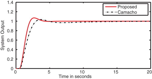
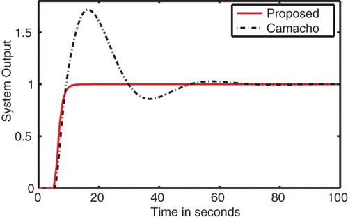
To validate the performance proposed controller, unit step change is applied to the system at time t=0. The system output, control input and sliding surface are shown in Figures 1(a), (b) and 1(c), respectively. Form Figure 1, it can be seen that the proposed controller produces smooth response with less and smooth control efforts while the response produced by Camacho et al.’s controller results in heavy overshoot. It can also be seen that with proposed controller the system reaches the sliding surface quite earlier as compared to that of Camacho's controller. This reduces the time of reaching phase and improves robustness. To verify the robustness of the proposed controller against parametric uncertainty, 20% uncertainty is added to all time constants. Figure 2 shows the comparison of the responses produced by the proposed and Camacho et al.’s controllers. From Figure 2, it can be seen that the proposed controller produces satisfactory results under the effect of parametric uncertainty while the response produced by Camacho et al.’s controller is sluggish.

Figure 1. System output, control signal and sliding surface for Example 1. (a) System output. (b) Control signal. (c) Sliding surface.

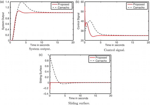
Figure 2. System output for Example 1 under 20% uncertainty.

4.2. Example 2

Consider a fifth-order system with OLTF (Chen & Peng, 2005) The continuous time-state model matrices are The discrete time-state model matrices for a sampling period of 1 s are The matrices Q and R are chosen as The sliding surface parameter matrix K, the switching gain k_sw in Equation (11) and the boundary layer constant β in tanh function are respectively.

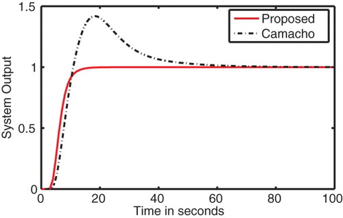
To validate the performance proposed controller, unit step change is applied to the system at time t=0. The system output, control input and sliding surface are shown in Figures 3(a), (b) and 3(c), respectively. Form Figure 3, it can be seen that the performance of the proposed controller is better than the performance produced by Camacho et al.’s controller. Also the control efforts required are less and smooth as compared to Camacho et al.’s controller. It can also be seen that with the proposed controller the system reaches sliding surface quite earlier as compared to that of with Camacho's controller. This reduces the time of reaching phase and improves robustness. To verify the robustness of the proposed controller against parametric uncertainty, 20% uncertainty is added to all time constants. Figure 4 shows the comparison of the responses produced by the proposed and Camacho et al.’s controllers. From Figure 4, it can be seen that the proposed controller produces satisfactory results under the effect of parametric uncertainty while the response produced by Camacho et al.’s controller has heavy overshoot.

Figure 3. System output, control signal and sliding surface for Example 2. (a) System output. (b) Control signal. (c) Sliding surface.

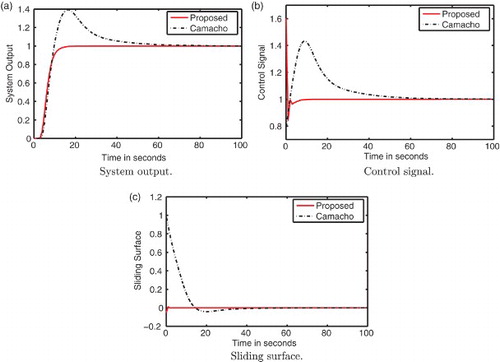
Figure 4. System output for Example 2 under 20% uncertainty.

4.3. Example 3

Consider a fourth-order system with OLTF (Camacho et al., 2007) The continuous time-state model matrices are The discrete time-state model matrices for the sampling period of 1 s are

The matrices Q and R are chosen as The sliding surface parameter matrix K, the switching gain k_sw in Equation (11) and the boundary layer constant β in tanh function are respectively.

To validate the performance proposed controller, unit step change is applied to the system at time t=0. The system output, control input and sliding surface are shown in Figures 5(a), (b) and 5(c), respectively. Form Figure 5, it can be seen that the performance of the proposed controller is better than the performance produced by Camacho et al.’s controller. Also the control efforts required are less and smooth as compared to Camacho et al.’s controller and further it can be seen that with the proposed controller the system reaches the sliding surface quite earlier as compared to that of Camacho's controller. This reduces the time of reaching phase and improves robustness.. To verify the robustness of the proposed controller against parametric uncertainty, 20% uncertainty is added to all time constants. Figure 6 shows the comparison of the responses produced by the proposed and Camacho et al.’s controllers. From Figure 6, it can be seen that the proposed controller produces satisfactory results under the effect of parametric uncertainty while the response produced by Camacho et al.’s controller has heavy overshoot.

Figure 5. System output, control signal and sliding surface for Example 3. (a) System output. (b) Control signal. (c) Sliding surface.

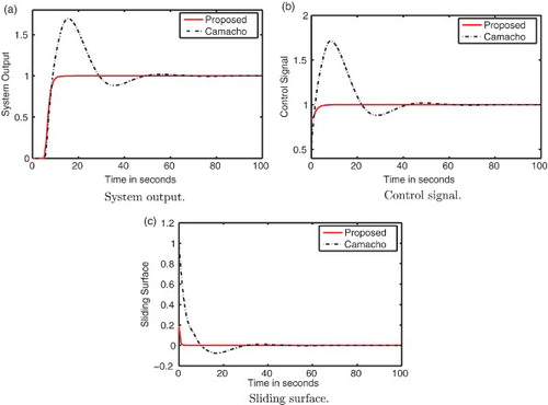
Figure 6. System output for Example 3 under 20% uncertainty.

5. Conclusions

This paper presents an optimal sliding surface combined with a delay ahead predictor to design DSMC for systems with parametric uncertainty. The optimal sliding surface is designed by minimizing the quadratic performance index. The stability condition is derived using the Lyapunov approach. The performance of the proposed controller is validated for nominal and parametric uncertain systems. Simulation results show that the proposed SMC strategy produces satisfactory results with less and smooth control efforts and is effective and promising in the control of uncertain time-delay systems. The presented controller will practically be useful in process control systems where there is considerable delay in the system model. If the delay is approximated by the delay approximation methods available in the literature, the parametric uncertainty (plant–model mismatch) increases and the control system performance is degraded due to lack of robustness. The proposed algorithm coupled with a decoupler can be extended for the control of multi-variable systems with time delay using multi-loop single input single output controller approach.

REFERENCES

- Boulkroune, A., & M'Saad, M. (2012). Fuzzy adaptive observer-based projective synchronization for nonlinear systems with input nonlinearity. Journal of Vibration and Control, 18(3), 437–450. doi: 10.1177/1077546311411228
- Boulkroune, A., M'Saad, M., & Chekireb, H. (2010). Design of a fuzzy adaptive controller for MIMO nonlinear time-delay systems with unknown actuator nonlinearities and unknown control direction. Information Sciences, 180, 5041–5059. doi: 10.1016/j.ins.2010.08.034
- Boulkroune, A., M'Saad, M., & Farza, M. (2011). Adaptive fuzzy controller for multivariable nonlinear state time-varying delay systems subject to input nonlinearities. Fuzzy Sets and Systems, 164, 45–65. doi: 10.1016/j.fss.2010.09.001
- Camacho, O., Rojas, R., & Gabin, V. G. (2007). Some long time delay sliding mode control approaches. ISA Transactions, 46, 95–101. doi: 10.1016/j.isatra.2006.06.002
- Camacho, O., & Smith, C. A. (2000). Sliding mode control: An approach to regulate chemical processes. ISA Transactions, 39, 205–218. doi: 10.1016/S0019-0578(99)00043-9
- Camacho, O., Smith, C. A., & Moreno, W. (2003). Development of an internal model sliding mode controller. Industrial Engineering Chemistry Research, 42, 568–573. doi: 10.1021/ie010481a
- Chen, C.-T., & Peng, S.-T. (2005). Design of a sliding mode control system for chemical processes. Journal of Process Control, 15, 515–530. doi: 10.1016/j.jprocont.2004.11.001
- Chen, M., Donghua Zhou, D., & Shang, Y. (2004). A simple time-delayed method to control chaotic systems. Chaos, Solitons & Fractals, 22, 1117–1125. doi: 10.1016/j.chaos.2004.03.021
- Gao, W., Wang, Y., & Homaifa, A. (1995). Discrete-time variable structure control systems. IEEE Transactions on Industrial Electronics, 42(2), 117–122. doi: 10.1109/41.370376
- Garcia, J. P. F., Silva, J. J. F., & Martins, E. S. (2005). Continuous-time and discrete-time sliding mode control accomplished using a computer. IEE Proceedings Control Theory and Applications, 152(2), 220–228. doi: 10.1049/ip-cta:20041129
- Golo, G., & Milosavljevi, C. (2000). Robust discrete-time chattering free sliding mode control. Systems and Control Letters, 41, 19–28. doi: 10.1016/S0167-6911(00)00033-5
- Hu, J., Chu, J., & Su, H. (2000). SMVSC for a class of time-delay uncertain systems with mismatching uncertainties. IEE Proceedings Control Theory Applications, 147, 687–693. doi: 10.1049/ip-cta:20000802
- Khandekar, A. A., Malwatkar, G. M., Kumbhar, S. A., & Patre, B. M. (2012). Continuous and discrete sliding mode control for systems with parametric uncertainty using delay-ahead prediction. Twelfth IEEE Workshop on Variable Structure Systems, Mumbai, India.
- Khandekar, A. A., Malwatkar, G. M., & Patre, B. M. (2013). Discrete sliding mode control for robust tracking of higher order delay time systems with experimental application. ISA Transactions, 52(1), 36–44. doi: 10.1016/j.isatra.2012.09.002
- Mihoub, M., Nouri, A. S., & Abdennour, R. B. (2009). Real-time application of discrete second order sliding mode control to a chemical reactor. Control Engineering Practice, 17, 1089–1095. doi: 10.1016/j.conengprac.2009.04.005
- Milosavljevic, C. (1985). General conditions for the existence of a quasi-sliding mode on the switching hyperplane in discrete variable structure systems. Automation and Remote Control, 3, 36–44.
- Ogata, K. (2003). Discrete Time Control Systems (2nd ed.). New Jersey: Prentice Hall.
- Roh, Y. H., & Oh, J. H. (1999). Robust stabilization of uncertain input-delay systems by sliding mode control with delay compensation. Automatica, 35, 1861–1865. doi: 10.1016/S0005-1098(99)00106-5
- Roh, Y. H., & Oh, J. H. (2000). Sliding mode control with uncertainty adaptation for uncertain input-delay systems. International Journal of Control, 73, 1255–1260. doi: 10.1080/002071700417894
- Sira-Ramirez, H. (1991). Non-linear discrete variable structure systems in quasi-sliding mode. International Journal of Control, 54, 1171–1187. doi: 10.1080/00207179108934203
- Utkin, V. I. (1992). Sliding Modes in Control and Optimization. Berlin: Springer.
- Wang, Q.-G., Lee, T.-H., Fung, H.-W., Qiang, B., & Zhang, Y. (1999) PID tuning for improved performance. IEEE Transactions on Control System Technology, 7(4), 457–465. doi: 10.1109/87.772161
- Zhang, T. P., & Ge, S. S. (2007). Adaptive neural control of MIMO nonlinear state time-varying delay systems with unknown dead-zones and gain signs. Automatica, 43(6), 1021–1033. doi: 10.1016/j.automatica.2006.12.014