A measurement-based technique for designing fixed-order RST controllers and application to a coupled water tank system

Abstract

This paper addresses the control design problem for unknown linear single-input single-output systems using a set of measurements. In standard control methods, controllers are designed on the basis of a mathematical model. Such a mathematical model, which describes the behavior of the system, can be developed using either physical laws or measured data. However, due to the complex dynamics of many physical systems, some prior assumptions are usually made to build simplified models. The efficacy of such model-based control techniques depends greatly on the quality of models used. Hence, data-based control design methods appeared as an alternative to model-based methods. Such data-based techniques are powerful in the sense that no mathematical model is needed for controller design. In this paper, we propose an approach that uses frequency response data to directly design controllers without going through any modeling stage. The main idea of our proposed method is to design polynomial RST controllers, for which the closed-loop frequency response fits a desired frequency response that describes some desired performance specifications. This problem is formulated as an error minimization problem, which can be solved using efficient optimization algorithms. The main feature of our proposed control approach is that it enables the designer to pre-select the controller structure, which allows the design of low-order controllers. Moreover, this control design approach does not depend on the increasing order and complexity of the system. An application to water level control of a coupled tank system is presented to validate and illustrate the efficacy of the proposed approach.

Keywords:

• measurement-based control
• polynomial RST controller
• low-order controller
• unknown dynamical systems
• error minimization

1. Introduction

The increasing complexity of large-scale industrial systems motivates the theoretical and practical developments of efficient modeling and control algorithms. Traditional control design approaches are often based on mathematical models that approximate the behavior of the physical system. Such mathematical models can be obtained using physical laws or via measurement-based system identification techniques. Process modeling of complex systems based on physical laws usually leads to large and high-order sets of algebraic or differential equations which can be difficult to obtain and solve. The identification process based on measured data, on the other hand, usually relies on some prior assumptions such as model structure and order, which are often unavailable or subject to uncertainties. Hence, the complexity and errors associated with such mathematical models increase the difficulty of the control design task and may lead to degradation of the closed-loop performance (Athans, Rohrs, Valavani, & Stein, 1982; Ioannou & Kokotovic, 1984). To avoid such a problem and maintain some desired closed-loop performance, data-based control design methods can be used instead of model-based design techniques. The principle of such data-based control approaches is to directly design controllers using a set of measurements carried out on the system, without explicitly using any mathematical model.

Data-based control design techniques are very useful in many practical control applications, where obtaining a suitable model that perfectly characterizes the behavior of the system is a very difficult task. In data-based control methods, measurements used in the control design process can be given in either time domain or frequency domain. Based on time-domain data, some approaches to design fixed-order controllers for model reference and tracking problem have been presented in Rojas, Flores-Alsina, Jeppsson, and Vilanova (2012), Rojas and Vilanova (2012), Hou and Jin (2011), Park and Ikeda (2004), Yasumasa, Duanm, and Ikeda (2005), Hjalmarsson, Gevers, Gunnarsson, and Lequin (1998), Campi, Lecchini, and Savaresi (2002) and Karimi, Miskovic, and Bonvin (2004). Measurement-based frequency-domain control techniques are often based on the frequency response of the plant which is assumed to be available or can be measured experimentally using a set of input/output measurements. Such an assumption is often valid in many practical applications. In Keel and Bhattacharyya (2008) and Kallakuri, Keel, and Bhattacharyya (2011), it has been shown that the entire set of stabilizing proportional-integral-derivative (PID) controllers can be obtained using only the frequency-domain data. Horowitz (1993) presented the quantitative feedback theory approach which is based on loop-shaping in the Nichols chart. A new measurement-based modeling technique, which is used for controller design, has been developed in Datta et al. (2013). Garcia, Karimi, and Longchamp (2006, 2003) utilized frequency-domain data to design controllers so that some desired closed-loop performance measures are satisfied. The design problem addressed in Garcia et al. (2006, 2003) has been formulated as a nonlinear nonconvex optimization problem and solved through a local gradient-based iterative algorithm. However, the fact that such an iterative algorithm is based on the computation of the gradient and Hessian of the objective function, it may fail to achieve the global optimum solution. Using frequency-domain data, den Hamer (2010) and Karimi and Galdos (2010) proposed a technique to design controllers such that the infinity norm of weighted sensitivity functions is minimized. Such a data-based design technique requires the selection of some weighting functions to establish the desired performance specifications, which is generally cumbersome and often based on the trial-and-error methods.

In this paper, we aim to design fixed-structure controllers for linear time-invariant signal-input signal-output (SISO) systems based only on frequency response data of the plant. Here, we are particularly interested in the design of polynomial RST controllers. The polynomials R and S allow us to create a feedback control loop, whereas the polynomial T is introduced in the feedforward to improve the reference tracking. The principle of our proposed control design method is to find suitable values of the polynomial coefficients of the RST controller so that the error between the measured frequency response of the closed-loop system and the desired frequency response is minimized over a finite range of frequencies. The main advantage of our proposed method is that it is possible to impose a priori the order of the polynomials R, S and T, which allows for the design of low-order RST controllers. Such low-order RST controllers allow us to avoid implementation problems due to computational limitations. Another feature of such a proposed control method is that the control design problem is solved through a global optimization algorithm that does not require the computation of the gradient and Hessian of the objective function. Moreover, since the only needed information about the plant is the frequency response data, the design process does not depend on the order, time delay or complexity of the plant. Due to its simplicity and ability to avoid the problem of under-modeling, the proposed approach can be very useful to successfully control linear SISO systems.

The paper is organized as follows. Section 2 is devoted to the formulation of the measurement-based RST controller design problem. The approach for designing RST controllers using a set of measurements is presented in Section 3. To experimentally validate the efficacy of the proposed method, a practical application to water level control of a coupled tank system is given in Section 4. Finally, Section 5 includes some concluding remarks.

2. Problem statement

Consider the control system configuration shown in Figure 1, where an unknown SISO linear system is controlled by an RST controller. H_cl(s) denotes the transfer function of the closed-loop system. The closed-loop scheme involves the following signals:

• y_c(t) is the reference input,

• y(t) is the output signal,

• u(t) is the input control signal, and

• ε(t) is the tracking error.

Fig. 1. RST controller for an unknown linear system.

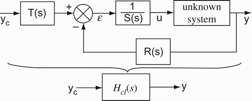
The choice of RST controllers in this paper is based on the fact that they have a more general structure. For instance, PID controllers are only a particular case of RST controllers, where R(s)=T(s) and S(s) are selected as second- and first-order polynomials, respectively. The design problem is to find the polynomials R, S and T of the controller for which some desired closed-loop performance specifications are satisfied. Suitable polynomials of the RST controller can be obtained using a mathematical model that perfectly describes the plant characteristics. However, as outlined in the introduction section, obtaining an accurate plant model is a very challenging task in many practical applications due to complex dynamics of the plant. Toward this end, we aim here to skip the modeling step and directly design RST controllers based on a set of measure data. This idea of data-based control design is motivated by the fact that difficulties and issues related to the modeling process are avoided. The proposed data-based methodology is of great importance to improve the operation of many practical applications, where reliable models are unavailable or difficult to obtain. Here, we assume that a set of input/output measurements can be collected to derive the frequency response of the plant over a set of distinct frequencies . Based on frequency response data of the plant, an RST controller can be designed to guarantee some desired closed-loop system performance specifications. Next, the proposed measurement-based RST control design methodology is presented.

3. Controller design method

In this section, we aim to design low-order RST controllers ensuring some performance measures for the closed-loop system given in Figure 1. The RST controller will be computed using only measurements without introducing any intermediate step of identification in the design process. Consider an RST controller with fixed-order polynomials as follows:

where a_i, b_l and c_d (for i=0, … , n, l=0, … , m and d=0, … , p) are the coefficients of the three polynomials R(s), S(s) and T(s), respectively. Here, it is assumed that m≥n≥p. Let be a vector containing the parameters of the RST controller. The control design problem is to find suitable values of the polynomial coefficients θ for which the closed-loop frequency response is very close to a desired closed-loop frequency response denoted by H*(jw_k), which meets some desired performance measures, over a sufficient range of frequencies, w_k, k=1, … , N. The range of frequencies is selected such that sufficient information about the frequency response of the system can be extracted. To this end, measurements may need to be collected over a sufficient range of frequencies with different frequency increments. Fine frequency increments are usually needed near the ranges of frequencies that exhibit rapid changes, where resonance and antiresonance phenomena occur. Over the ranges of frequencies where the variations of the frequency response are very slow, larger frequency increments can be selected.

Throughout this paper, we will define any frequency response in the Nyquist plane in terms of its real and imaginary parts. Assume that the frequency response of the plant, denoted by G(jw_k), can be expressed at each frequency w_k, k=1, 2, … , N, in terms of its real and imaginary parts R_G(w_k) and I_G(w_k), respectively, as follows:

For each frequency w_k, the imposed polynomials R, S and T can be defined in the Nyquist plane using their real and imaginary parts as follows:

where ℜ and ℑ indicate the real and imaginary parts of complex numbers.

Using Equations (2) and (3), the frequency response of the closed-loop system (Figure 1) can be expressed for all frequencies as follows:

which can be written in the following form:

where the real and imaginary parts of the closed-loop frequency response are functions of R_G(w_k), I_G(w_k) and the parameter θ of the RST controller.

Also, let us assume that the frequency response corresponding to a desired closed-loop system can be written as follows:

This desired frequency response (6) describes the performance expected for the closed-loop system.

Let be the error between the computed frequency response and the desired frequency response H*(jw_k), at the frequency w_k, k=1, 2, … , N. It is defined as follows:

which can be written as follows:

Hence, our problem can be reformulated as follows: find suitable values of the RST controller parameter θ* so that the following criterion J defined by the integral of the squared error over the selected range of frequencies w_k, k=1, 2, … , N, is minimized:

where ρ_k, are the penalty coefficients and is the complex conjugate of the error that is defined in Equation (8). Criterion (9) can be rewritten as follows:

The above problem is a nonlinear (with respect to θ) nonconvex optimization problem, in which a globally optimum solution can be found by applying global optimization approaches. In the area of optimization, various methods (deterministic and stochastic) have been developed to solve global optimization problems (Floudasa, Akrotirianakisa, Caratzoulasa, Meyera, & Kallrathb, 2005; Horst & Tuy, 1996; Kennedy & Eberhart, 1995; Schaffler, 2012; Shi & Eberhart, 1999; Sotiropoulos, Stavropoulos, & Vrahatis, 1997; Torn & Zilinskas, 1989). Depending on context, each approach has its own particular advantages and disadvantages. The particle swarm optimization (PSO) is a stochastic algorithm inspired by social behavior of animals such as bird flock and fish school (Kennedy & Eberhart, 1995; Shi & Eberhart, 1999). It has been widely used to solve global optimization problems mainly due to its flexibility and simplicity of implementation as well as its ability to deal with large search space and relatively high number of parameters without the need for direct evaluation of gradients. Table 1 summarizes the PSO algorithm used to solve the control design problem (10). The PSO algorithm requires a search space, , for the RST controller parameters. A set of M particles (called population or swarm) is first randomly generated in such a search space, with an initial position vector, , and velocity vector, . The position associated with each particle represents a possible solution of the above control design problem. Each particle, i=1, … , M, moves iteratively in the search space, , toward its best previous visited position, , and toward the global best recorded position, θ^gb, of the swarm (see step 6.a). The PSO algorithm utilizes some constants to update the position of each particle. c₁∈[1.7, 2] (resp. c₂∈[1.7, 2]) is the cognitive factor (resp. social factor) that accelerates each particle from its current position toward its best recorded position (resp. the global best position). is the inertia factor, while γ₁ and γ₂ are random numbers in the range [0, 1]. After a finite number of iterations, it=it_max; defined by the user, the global optimum solution is selected to be (step 7).

Table 1 PSO algorithm for solving the design problem (10).

Remark 3.1 In some cases, where the plant is characterized by a significant delay or is of infinite dimension, it is difficult to achieve a good matching between the closed-loop and desired frequency responses using low-order RST controllers. Hence, in such a situation, the user should use higher degree for the polynomials of the RST controller given in Equation (1) and reapplied again the PSO algorithm.

Remark 3.2 In this contribution, only SISO systems are considered. However, the proposed method can be extended to multiple-input multiple-output (MIMO) systems. In such an MIMO case, it is required to collect a large number of measurements from the MIMO plant. Moreover, the complexity of the multivariable controller computation increases as the dimension of the MIMO system increases.

One important issue related to the measurement-based control design is closed-loop system stability. Hence, a posteriori check of closed-loop stability is of great importance. Closed-loop stability can be analyzed based on the frequency response of stable open-loop systems (Keel & Bhattacharyya, 2010; Mohsenizadeh, Darbha, Keel, & Bhattacharyya, 2012). According to Keel and Bhattacharyya (2010) and Mohsenizadeh et al. (2012), the closed-loop system is stable if and only if the Nyquist contour of the stable open-loop system, traversed in the sense of growing frequencies (), does not encircle the critical point (−1, 0j). When the open-loop system is unstable, stability check of measurement-based control approaches requires knowledge of the number of unstable poles of the open-loop system, which is often not available. In such a situation, Sala and Esparza (2005) and Lanzon, Lecchini, Dehghani, and Anderson (2006) proposed to identify a model for the closed-loop system using available closed-loop frequency response data. Also, the stability analysis can be performed by assessing stability margins. This later can be done using gain and phase margins which are a good indicator of stability.

4. Application to a water coupled tank system

This section is mainly devoted to an experimental application of the proposed control design approach discussed in the previous section.

4.1. System description and specifications

The process to be controlled is a water coupled tank system which is widely available in industrial chemical applications, such as petrochemical processes. It consists of two coupled tanks, an upper tank T₁ and lower tank T₂, which are interconnected in series as shown in Figure 2. A pump driven by a DC motor thrusts water collected in a water basin (the main water reservoir) to the tank T₁. The water level in each tank is measured by means of a pressure sensor. Here, our control objective of this experiment is to maintain the water level l₂ in the tank T₂ at a desired value by manipulating the input voltage of the pump. The following hardware and software are used for the experimental setup:

• coupled tank plant;

• PC and a Quanser data acquisition board (Q8-USB);

• Quanser power module used to amplify the input signal provided by the controller;

• Quarc-Simulink software used for the implementation of the controller.

Fig. 2. Synoptic of the experimental setup.

Hence, we focus here on designing a measurement-based RST controller that guarantees stability and meets the following closed-loop design specifications for a unit step input: closed-loop behavior with small overshoot, settling time of about 100 s, and small steady-state error.

4.2. Controller design

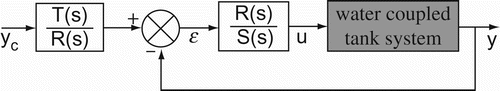
Here, the measurement-based control approach presented in the previous section is utilized to design an RST controller that ensures the above closed-loop performance requirements for the water coupled tank system. Let us consider the control scheme with an RST controller as shown in Figure 3, which can be directly obtained from the control configuration presented in Figure 1.

Fig. 3. RST controller for the water coupled tank system.

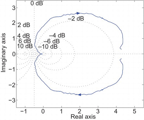
The frequency of interest considered in this application ranges from 0 to 0.1 Hz. First, a harmonic analysis is performed on the system (whose input and output are the input voltage applied to the pump and the water level in the tank T₂, respectively) in order to derive its frequency response, i.e. . The Nyquist response of the controlled system is computed based on a set of input/output measurements carried out at a finite set of distinct frequencies  rad/s (for ). The resulting Nyquist plot is shown in Figure 4.

Fig. 4. Experimental Nyquist plot of the water coupled tank system.

In this application, we consider a fixed-order RST controller structure with a low degree for each polynomial R, S and T, to simplify the design and implementation and the controller. Let us assume that all of these polynomial are of first order as follows:

We have chosen S(s)=s in order to have an integral action in the feedback control loop. Nevertheless, according to the control system configuration given in Figure 3, the use of an integrator in the feedback control loop is not enough to ensure zero steady-state error. Hence, in addition to the integral action, the parameters a₀ and d₀ must be equal (i.e. a₀=d₀) in order to guarantee a unity static gain (zero steady-state error). Thus, the polynomials in Equation (11) can be written as follows:

where a₀, a₁ and d₁ are the parameters of the RST controller to be tuned. Based on the measured frequency response of plant and that of the polynomials (12), the frequency response, , of the closed-loop system at each frequency can be derived using the relation (4) as follows:

A reference model that describes the desired closed-loop behavior can be selected as

where the parameters K and τ are designed to satisfy the desired closed-loop performance specifications outlined above as follows:

• to ensure a zero steady-state error, the gain K should be chosen equal to one,

• to achieve the desired settling time, the time constant should be selected as  s.

It is worth noting that the reference model above is considered here to be first-order transfer function only for simplicity reasons. However, second- or high-order reference models that describe the desired closed-loop performance can still be used.

The frequency response of the reference model at each frequency is given by

Suitable values of the coefficients a₀, a₁ and d₁ can be obtained by minimizing the cost function (10), which depends on the quadratic error between the closed-loop frequency response (13) and the reference model frequency response (15), over the set of frequencies w_k, . In this practical example, a number of M=50 particles is selected and the following parameter values have been used to solve the optimization problem (10): ρ_k=1, φ=0.1, c₁=2, c₂=2 and max_it=100. After applying the algorithm presented in Table 1, the following RST controller parameters are obtained: , a₁=2.136 and d₁=0.194. These values of the controller parameters are used for the implementation of the RST controller (Figure 3).

4.3. Closed-loop stability analysis

Before experimentally validating the closed-loop response when the designed RST controller is implemented, it is important to check the stability of the resulting closed-loop system (Figure 3). Hence, since the open-loop system is stable, we propose here to perform a closed-loop stability check based on the frequency response of the open-loop system as proposed in Keel and Bhattacharyya (2010) and Mohsenizadeh et al. (2012). The Nyquist plot of the open-loop system over all set of frequencies, is shown in Figure 5.

Fig. 5. (a) Nyquist plot of the open-loop system. (b) Zoom on the part of the Nyquist plot around the critical point.

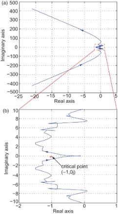
It is clear, according to Figure 5(a) and 5(b), that the Nyquist contour of the open-loop system, traversed in the sense of growing frequencies (), does not encircle the critical point (−1, j0). Hence, based on results in Keel and Bhattacharyya (2010) and Mohsenizadeh et al. (2012), the designed RST controller stabilizes the closed-loop system.

4.4. Experimental results

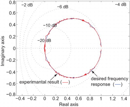
The computed RST controller (12) was placed in the unity feedback configuration as in Figure 3. Then, a harmonic analysis is performed by applying a reference input signal. This later is composed of a sinusoidal signal superimposed on a DC offset component. The DC offset component is about 15 cm, whereas the sinusoidal signal with a unity amplitude is applied using the same set of frequencies . The obtained experimental results of the closed-loop system are drawn in the Nyquist plane as depicted in Figure 6, which also shows the desired frequency response, H*(jw) (see Equation (15)). As shown in Figure 6, the experimental closed-loop frequency response is very close to the desired frequency response, which means that the implemented RST controller achieves the required performance for the water coupled tank system.

Fig. 6. Experimental and simulation Nyquist plots of the closed-loop system (H_cl(jw) and H*(jw)).

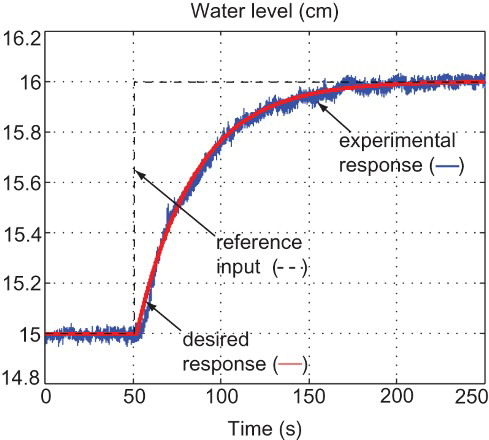
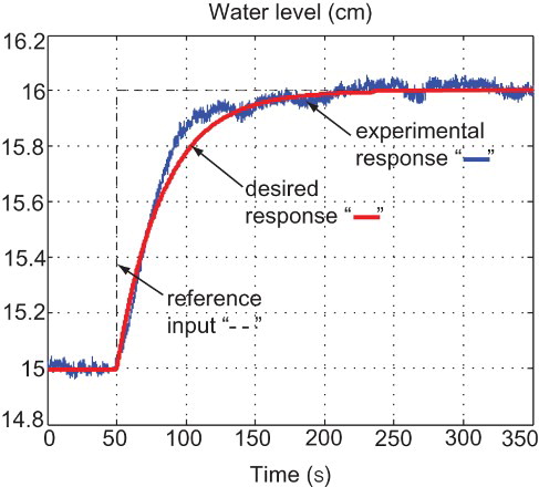
Using an initial water level in tank T2 of 15 cm, Figure 7 shows the experimental closed-loop response when a step reference input of magnitude 16 cm is used. The same figure shows the step response of the reference model (14) to show the difference between the experimental step response and the desired step response. As shown in Figure 7, the difference between both responses is small. Thus, the controller has achieved the desired closed-loop performance in terms of overshoot, settling time (which is about  s) and steady-state error.

Fig. 7. Comparison between the experimental and desired closed-loop step responses.

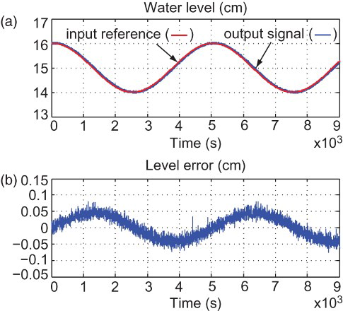
We have also evaluated the tracking performance of the water coupled tank system when a sinusoidal input reference trajectory (having a frequency of  Hz) is used. Figure 8(a) presents the experimental results obtained when the computed RST controller is applied, where it is clear that the output tracks the reference input quite well.

Fig. 8. Tracking characteristics with the RST controller.

Now, we attempt to solve the same problem as before using another structure for the RST controller. For that, we consider the design of the following RST controller with T(s)=R(s):

The design problem of this later RST controller is equivalent to the design of a proportional-integral (PI) controller C(s), where . We follow the same procedure as before to derive the corresponding controller parameters: a₀ and a₁. It has been found that minimizing the cost function (10) with penalty coefficients ρ_k=1 results in the following controller parameters: and a₁=0.212. The same procedure presented in Section 4.3 has been used to check the stability of the resulting closed-loop system when the PI controller (i.e. the RST controller given in Equation (16)) is applied. When the designed PI controller is implemented, the experimental frequency and step responses of the closed-loop system are shown in Figures 9 and 10, respectively. Figure 9 shows that the experimental frequency response is close to the desired frequency response. According to Figure 10, the implemented PI controller resulted in a closed-loop response that meets the desired design requirements. In fact, the achieved closed-loop performance can be described as follows: small overshoot, settling time about 105 ms which is acceptable in such an application and small static error of less than 5%. In this particular application, it has been found that the designed RST controller (12) provides an improved closed-loop performance over the designed PI controller (16).

Fig. 9. Experimental Nyquist plot of the closed-loop system with a PI controller compared to the desired response.

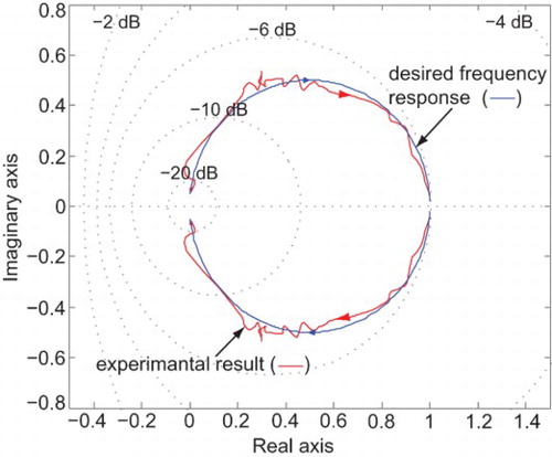
Fig. 10. Experimental closed-loop (with a PI controller) and desired step responses.

5. Conclusion

In this paper, we have addressed the problem of designing fixed-structure RST controllers for SISO linear systems using measured frequency-domain data. It has been shown that the design problem of polynomial RST controllers can be formulated as a minimization problem of the integral of the square error between the closed-loop frequency response and a desired frequency response, which meets some desired closed-loop performance specifications. The PSO algorithm has been used to solve such a design problem. Such an algorithm is able to deal with relatively high number of the polynomial coefficients of the RST controller. The proposed control design method allows us to design low-order RST controllers by simply imposing the degree of their polynomials. In addition, since no mathematical model is required, the controller design does not depend on the increasing order or complexity of the system. The proposed approach has been experimentally applied to control water level of a coupled tank system. The experimental results obtained have demonstrated the efficacy of the proposed approach to design fixed-structure RST controllers for unknown systems using frequency-domain data. In addition, closed-loop stability check based on a frequency response approach has been established. One of our future research works will be focused on designing a robust and adaptive measurement-based controller for unknown uncertain systems.

This work was made possible by NPRP grant NPRP09-1153-2-450 from the Qatar National Research Fund (a member of Qatar Foundation). The statements made herein are solely the responsibility of the authors.

REFERENCES

- Athans, M., Rohrs, C. E., Valavani, L., & Stein, G. (1982). Robustness of adaptive control algorithms in the presence of unmodeled dynamics. 21st IEEE Conference on Decision and Control, Orlando, FL, 8–10 December, pp. 3–11.
- Campi, M. C., Lecchini, A., & Savaresi, S.M. (2002). Virtual reference feedback tuning: A direct method for the design of feedback controllers. Automatica, 38, 1337–1346. doi: 10.1016/S0005-1098(02)00032-8
- Datta, A., Layek, R., Nounou, H., Nounou, M., Mohsenizadeh, N., & Bhattacharyya, S.P. (2013). Towards data based adaptive control. International Journal of Adaptive Control and Signal Processing, 27, 122–135. doi: 10.1002/acs.2339
- Floudasa, C. A., Akrotirianakisa, I. G., Caratzoulasa, S., Meyera, C. A., & Kallrathb, J. (2005). Global optimization in the 21st century: Advances and challenges. Computers and Chemical Engineering, 29 1185–1202. doi: 10.1016/j.compchemeng.2005.02.006
- Garcia, D., Karimi, A., & Longchamp, R. (2003). Data-driven controller tuning based on a frequency criterion. 42nd IEEE Conference on Decision and Control, Maui, HI, 9–12 December, pp. 127–132.
- Garcia, D., Karimi, A., & Longchamp, R. (2006). Data-driven controller tuning using frequency domain specifications. Industrial and Engineering Chemistry Research, 45 4032–4042. doi: 10.1021/ie0513043
- den Hamer, A. J. (2010). Data-driven optimal controller synthesis: A frequency domain approach (PhD dissertation). Eindhoven University of Technology.
- Hjalmarsson, H., Gevers, M., Gunnarsson, S., & Lequin, O. (1998). Iterative feedback tuning: Theory and application. IEEE Control Systems Magazine, 18 26–41. doi: 10.1109/37.710876
- Horowitz, I. M. (1993). Quantitative feedback design theory (QFT). Boulder, CO: QFT publications.
- Horst, R., & Tuy, H. (1996). Global optimization: Deterministic approaches. Berlin: Springer.
- Hou, Z. S., & Jin, S.T. (2011). A novel data-driven control approach for a class of discrete-time nonlinear systems. Transactions on Control Systems Technology, 19 1549–1558. doi: 10.1109/TCST.2010.2093136
- Ioannou, P. A., & Kokotovic, P.V. (1984). Instability analysis and improvement of robustness of adaptive control. Automatica, 20 583–594. doi: 10.1016/0005-1098(84)90009-8
- Kallakuri, P., Keel, L. H., & Bhattacharyya, S.P.. (2011). Data based design of PID controllers for a magnetic levitation experiment. 18th IFAC World Congress, Milan, Italy, 28 August–2 September, pp. 10231–10236.
- Karimi, A., & Galdos, G. (2010). Fixed-order H∞ controller design for nonparametric models by convex optimization. Automatica, 46 1388–1394. doi: 10.1016/j.automatica.2010.05.019
- Karimi, A., Miskovic, L., & Bonvin, D. (2004). Iterative correlation-based controller tuning. International Journal of Adaptive Control and Signal Processing, 18 645–664. doi: 10.1002/acs.825
- Keel, L. H., & Bhattacharyya, S.P.. (2008). Controller synthesis free of analytical models: Three term controllers. IEEE Transaction on Automatic Control, 53 1353–1369. doi: 10.1109/TAC.2008.925810
- Keel, L. H., & Bhattacharyya, S.P.. (2010). A bode plot characterization of all stabilizing controllers. IEEE Transactions on Automatic Control, 55 2650–2654. doi: 10.1109/TAC.2010.2067390
- Kennedy, J., & Eberhart, R. (1995). Particle swarm optimization. Proceedings of the IEEE International Conference Neural Networks, vol. IV, Perth, Australia, 1942–1948.
- Lanzon, A., Lecchini, A., Dehghani, A., & Anderson, B.D.o. (2006). Checking if controllers are stabilizing using closed-loop data. 45th IEEE Conference on Decision and Control, San Diego, CA, 13–15 December, pp. 3660–3665.
- Mohsenizadeh, N., Darbha, S., Keel, L. H., & Bhattacharyya, S.P.. (2012). Model-free synthesis of fixed structure stabilizing controllers using the rate of change of phase. IFAC Conference on Advances in PID Control, Brescia, Italy, 28–30 March, pp. 745–750.
- Park, U. S., & Ikeda, M. (2004). Data-based stability analysis for linear discrete-time systems. 43rd IEEE Conference on Decision and Control, Atlantis, Bahamas, 14–17 December, pp. 1721–1723.
- Rojas, J. D., Flores-Alsina, X., Jeppsson, U., & Vilanova, R. (2012). Application of multivariate virtual reference feedback tuning for wastewater treatment plant control. Control Engineering Practice, 20 499–510. doi: 10.1016/j.conengprac.2012.01.004
- Rojas, J. D., & Vilanova, R. (2012). Data-driven robust PID tuning toolbox. 2nd IFAC Conference on Advances in PID Control, Brescia, Italy, 28–30 March, pp. 134–139.
- Sala, A., & Esparza, A. (2005). Extensions to “virtual reference feedback tuning: A direct method for the design of feedback controllers”. Automatica, 41 1473–1476. doi: 10.1016/j.automatica.2005.02.008
- Schaffler, S. (2012). Global optimization: A stochastic approach. New York: Springer.
- Shi, Y., & Eberhart, R.C. (1999). Empirical study of particle swarm optimization. Proc. IEEE International Conference on Evolutionary Computation, Washington, DC, July, 1945–1950.
- Sotiropoulos, D. G., Stavropoulos, E. C., & Vrahatis, M.N.. (1997). A new hybrid genetic algorithm for global optimization. Nonlinear Analysis, Theory, Methods and Applications, 30 4529–4538. doi: 10.1016/S0362-546X(96)00367-7
- Torn, A., & Zilinskas, A. (1989). Global optimization. Berlin: Springer-Verlag.
- Yasumasa, F., Duanm, Y., & Ikeda, M. (2005). System representation and optimal tracking in data space. 16th IFAC World Congress, Prague, Czech Republic, 4–8 July.