Application of distributed control on a large-scale production/ distribution/inventory system

ABSTRACT

Distributed control can be used against centralized control in terms of computational burden and functional issues. The current paper focuses on offline application of distributed control (by receding horizon approach) to a large-scale production/distribution/inventory network or in the other words, a supply chain system. In some industries, long-term demands are given or forecasted regarding product nature and therefore, the use of online repetitive control is unnecessary and non-economic. Of course, for avoiding wrong demands, a demand inspection unit (online adaptation unit) can be considered that evaluates applied demands in definite time periods and in fact makes a quasi-online concept. Each node is controlled separately by a local full-time receding horizon controller and then gives a logistical programme to the decision-maker or node manager and shares its information with neighbour nodes in a cascade organization. This method leads to an effective economic distributed solution for large-scale supply chains with certain variations.

KEYWORDS:

• Supply chain management system
• receding horizon control
• distributed control
• logistical programme
• inventory
• demand

1. Introduction

The decision for producing a product begins from customers. Customers request a favourable commodity by visiting retailers in a distribution network and this motive is transferred to manufacturers to meet the opportunity through a network of suppliers, manufacturers, distributors, and retailers. This network is named a production/distribution/inventory system because it consists of an inventory management part, a logistic network, and production programming. In a more general concept, this network is recognized namely as the supply chain management system. In a supply chain, a set of decision-maker facilities (suppliers, manufacturers, warehouses, distributors, and retailers) cooperate for getting the demands or forecasting them, ordering, procuring materials or outsourcing parts of the production procedure, manufacturing or assembling and finishing final products, stocking inventory, transporting, and finally delivering the final products to customers. Supply chains should be programmed by an efficient manager (or set of managers) who applies previous experiences with modern methods. This combination is named a supply chain management system and runs two processes of decisions and actions as orders and shipments.

In some of the industries, such as industries that have a definite customer or contract, change in demand pattern across time rarely happens. In the supply chain of these products, in a specific time such as at the beginning time of contract or at the beginning time of production, a correct pattern of customer demand is forecasted by famous methods, and production planning goes ahead for having a suitable customer demand planning. The problem is solved offline in this time as zero time and its output is used for programming and scheduling shipments between supply chain entities, manufacturing planning, and holding or managing inventory volumes. Therefore, in this situation, the optimization problem of the supply chain management system considering the required constraints is just solved for zero time and then production, warehousing, and distribution plans are given to related persons, managers, and employers of each division.

The programming and control (decision-making) of supply chain can be made by different methods, such as deterministic analytical models, stochastic analytical models, and simulation models coupled with desired optimization objectives and network performance measures (Beamon, 1998).

To employ control methods with prediction abilities is very suitable for supply chain management systems because decision prediction by looking to future demand exists inherently. Receding horizon control (RHC) is one of them that uses the rolling horizon concept and constrained steady-state model-based optimization among prediction and control horizons to find out a practicable solution with reasonable computational volumes. In recent years, numerous research have been conducted in this field and some of them are addressed in the reference list (Dunbar & Desa, 2007; Mastragostino, Patel, & Swartz, 2014; Subramanian, Rawlings, & Maravelias, 2014).

In this paper, a discrete time difference model is used that shows normal relationships between units in a production–delivery chain (Seferlis & Giannelos, 2004). This model has a modular structure and is extensible to any large-scale supply. Also, an RHC method is used beside the model for considering predictions and uncertainties (Chopra & Meindl, 2004; Wang & Rivera, 2005). In large-scale supply chains, distributed structures are used for decreasing input dimensions and complexity of solution and also operational issues (Sarimveis, Patrinos, Tarantilis, & Kiranoudis, 2008). The considered solution is based on distributed RHC in order to apply past and present control actions in future predictions (Camacho & Bordons, 2004; Findeisen, Allgöwer, & Biegler, 2011). This method decreases computational complexity and fault damages.

The paper shows an offline application of distributed RHC for an uncompleted supply chain system including one plant, two warehouses, four distribution centres, and four retailers. In uncompleted supply chains, node connection is not complete; thus, downstream nodes have no connection with all of the neighbour nodes in the upstream echelon. Also, a demand inspection unit is designed to evaluate applied demands in definite time periods and so by this way, the solution is equipped by a quasi-online adaptor algorithm. Each node is optimized separately by a local full-time receding horizon controller and then a specific programme is planned to keep safety inventory and satisfying customers. Finally, the simulations show the efficiency of this method in the field of easy operations and customer satisfaction with reasonable costs in facing unforeseen changes.

2. Inventory management system

The inventory management model with related upstream suppliers is described under concept of discrete time difference formulation, a complete modular and convenient with each type of multi-product, multi-echelon, multi-channel with specifying delays as individual parameter for each specific node and different demands. DP, P, RS, W, D, and R indicate the following parameters subsequently: a set of desired products manufactured at plants, plants, resources, warehouses, distributors, and retailers. The model is described as Equations (1)–(3) based on Figure 1. The model is categorized into three stages: production, distribution, and delivery, and pivotally shows the concept of production/distribution/inventory system in a supply chain. Safety inventories should be kept on warehouses and distributors and retailers. Of course, it is very economic that any inventory does not be stored as an ideal situation. Each defined echelon can include many dependent sub-echelons that they are defined as nodes of the network. A plant fabricates new products of semi-products or resources supplied by suppliers, or assembles semi-products and uncoupled devices. Finished products are shipped to warehouses and then are distributed, retailed, and delivered to final customers. In this procedure, some orders that are missed and that don't satisfy should be returned and reordered to upstream agents.

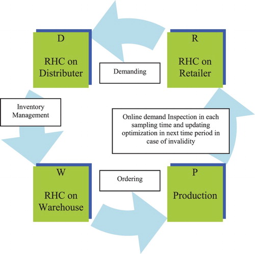
Figure 1. Quasi-online distributed RHC of a supply chain management system.

Control actions are taken at time periods on the bases of hours, days, weeks, and season and the length of the action should be selected based on dynamic characteristics of the supply chain, and the supply chain manager or decision-maker should be careful not to underestimate long period dynamics, because the effect of high-frequency variables may be omitted or ignored in optimization periods and calculations (Perea, 2007).

As mentioned, each echelon can be formed by some nodes and their number or indicator is addressed by k. There are neighbours for each specific node which are defined as downstream nodes, , because of their proximity to the plant echelon and upstream nodes, , because of their proximity to customers. Each node k is supplied by upstream nodes and supply downstream nodes by designed channels and subsequently. As mentioned, in the present work, there are no complete communication between nodes in neighbour echelons, and hence, transportation acts could not be started from all of the defined upstream neighbour nodes towards axial node k and then don't lead to all of the defined downstream neighbour nodes.

The following equations show a real interpretation of engagement between supply chain facilities based on an input/output analysis. These discrete time equations define supply and logistics procedures as product shipment between echelons and its cumulative effect on inventory accumulation at time instances t and t + 1. T is defined as the general time period and DP as desired products. The following equation represents inventory flows in warehouses and distributers where the inventory of product i in each node k, , at time instance (period) t + 1 is equal to the inventory of the same product in the same node at time instance t plus the transferred products of type i to node k from related upstream nodes through the transportation route , , delayed with the transportation lag at time instance t minus the delivered products of type i to downstream node from related upstream nodes through the transportation route , , at time instance t. (1)

The transportation lag is the delay factor defined as a multiple of the time period. The second and third equations specify product flows in retailer nodes. In the below equation, the inventory of product i in each typical retailer node k, , at time instance (period) t + 1 is equal to the inventory of the same product in the same node at time instance t plus the transferred products of type i to node k from related upstream nodes through the transportation route , , delayed with the transportation lag at time instance t minus delivered items to the customer, , at time instance t. (2)

The third equation defines back orders and their influences on customer satisfaction. The unsatisfied demand is indicated as labelled back orders based on product type, time period, and node number. (3)

Regarding this equation, , the back order of product i in node k at time instance t + 1 is equal to the back order of the same product in the same node at time instance t plus , the requested products of type i from node k, minus the delivered products of type i to the customer and lost orders of type i from node k, , at time instance t (Sterman, 2002).

3. Receding horizon control

There are two main elements in supply chain negotiations to access better efficiency. The first element is customer satisfaction and the second element is the cost problem. Customer satisfaction can be met by reducing back orders, meaning that maximum customer demand will be satisfied in the request period. The costs including warehousing, transportation, sharing networks, etc., should be controlled and optimized for achieving more profit RHC as a general form of state-space model predictive control methods can represent the fact that past and present control actions affect the future response of a supply chain management system. As previously mentioned, the discrete time models formulated by Equations (1)–(3) are forecasting tools of supply chain actions. They are used under the prediction horizon of a predictive optimizer (objective function) over time.

From the perspective of control science with the interpretation of the model, the state variables are defined as follows:

• The product inventory levels at stock nodes that are indexed by y.

• The back orders at retailer nodes indexed by BO.

Also, the input control variables are defined in two categories as follows:

• The products distributed by allowed transportation channels between nodes and echelons indexed by x.

• The delivered products to end users indexed by d.

In the current study, the output variables are considered as equivalent with the state variables.

Generally, in the RHC structure, there are two divisions: modelling (or model identification) and optimization. In each sampling time (or specified time duration), state-space model, parameters, disturbances, and uncertainties are identified and then a specified objective function is optimized by input control variables based on the model with defined prediction and control horizons (the prediction horizon to specify the influence of time for penalizing and subduing state and output variables and the control horizon to specify the influence of time for penalizing and subduing control and input variables and also related rates). Based on this procedure, in each sampling time (or specified time duration), the optimization problem is completely solved and then the first array of resultant input (or some of the first arrays) is saved and applied to the model, and all of the optimization and identification processes will continue in the next repetitive stages in future sampling times till the end of the simulation time (planning and operation duration) and finally will form a complete input.

In the available work, regarding the online nature of the receding horizon and also the effect of prediction on the efficiency of supply chain procedures, especially in the category of demands, a quasi-online distributed RHC for uncompleted supply chain management systems is developed. Distributed control has less computational burden and operational issues than centralized control. Of course, in fact, decentralized control efficiency should close to the ideal cooperation of centralized control. The focus is on long-term demand industries in which demands are given or forecasted for a long duration and don't change, or in a worst case situation, change in certain time intervals. It is completed depending on the product nature and, therefore, the use of online repetitive control is uneconomical.

The mentioned quasi-online method is based on a demand inspection or supervisory unit that is applied to an uncompleted supply chain system including one plant, two warehouses, four distribution centres, and four retailers. In this procedure, the optimization problem of each node in each echelon (that can be a retailer or a warehouse or a distributor) with the defined structure of local full-time receding horizon controllers and forecasted long-term demands is solved separately and completely. In zero time, in the first step, the first echelon (retailer) is solved and results are saved and common inputs are shared as measurable disturbances with upstream neighbour nodes in the upstream echelon. In the second step, the second echelon (distributor) is solved and results are saved and common inputs are shared as measurable disturbances with upstream neighbour nodes in the upstream echelon. In the third step, the third echelon (warehouse) is solved and results are saved. In the next stage, the automated inspection unit reviews and evaluates current demand and decides to issue license for the validity of results regarding inspections. In the case of invalidity, the steps should be repeated again by considering new demands.

The centralized objective function compliant with the discrete time model of supply chain management systems including four parts, such as inventory tracking, transportation penalty, back order, and transportation rate penalty, is described as follows (Miranbeigi, Moshiri, & Rahimi-Kian, 2014; Miranbeigi, Moshiri, Rahimi-Kian, & Razmi, 2015): (4)

In the above total penalty equation, P and C are sequentially the representatives of prediction horizon and control horizon. In the first term of the equation, inventory tracking, the inventory level in node k and for product i is penalized and directed towards a definite non-negative inventory level (regarding inventory capacity of node and current need) by penalty weight and over the prediction horizon. In the second part, transportation penalty, product quantities of type i transported throughout upstream node to downstream node (control inputs) are penalized to access a definite non-negative transportation level (regarding capacity of transportation network) by penalty weight and over the control horizon. The next term is related to back orders in retailer nodes and tries to zero it by penalty weight and over the prediction horizon. The final term penalizes deviations of transportation quantities between two successive times in a specified channel by weight and over the control horizon. This term also is named a move suppression term and is very useful for robustness and avoiding the bullwhip effect in a supply chain. The weight factors are selected according to a correct background of the system to recognize targets, appropriate speed, total costs, suitable rate of input changes, acceptable range of back-order rate, transportation delays, output response, and training procedures. As explained, a move suppression term increases robustness, but on the other hand it decreases response speed and adverse customer lead time. In addition, the desired points of inventory levels, setting the weights, selecting the horizons, demand forecasting, sharing information, cooperation procedures, applying delays with appropriate estimation, and move suppression term are similar to parts of puzzles that should be organized for having a comprehensive and effective trade-off. One of them can disturb or improve control of the supply chain management system.

The target level of transportation is considered to be about zero to access better profit, and total performance index equation (4) regarding local models (1)–(3) and decomposing the performance index to three local functions corresponding to each independent echelon and its related nodes is written as the below comprehensive cascade objective function: (5)

In this optimization problem, , and are sets of permissible time durations subsequently for retailer nodes, distributor nodes and warehouse nodes that show clearly distributed control and cascade regimes.

According to Figure 1, first of all, customer demands are forecasted by retailers or third-party predictors and then given to retailers as measurable disturbances. In this phase, complete RHC optimization problems of retailer nodes in the first echelon are locally minimized based on the inputs (entrance transportation quantities) regarding the first floor of the cascade object function described in Equation (5) and then the obtained common inputs are used as measurable disturbance for RHC of the distribution echelon. In next phase, in a farther step, distribution nodes receive the measurable disturbances and underpin optimization problems to produce logistics decisions of product transportation towards the end customer. They solve their complete RHC optimization problem and then share the coupled input information as measurable disturbance for RHC of the next echelon (warehouse). Warehouse echelon is the last decision field in the supply chain and similarly, their nodes solve their local complete RHC optimal control problem among the earlier defined horizons and finally, the rate of production by the plant will be indicated. After a complete scan of the supply chain management system, all of the decision quantities are known and are sent for application by node managers and then a demand inspection agent will review and evaluate demand patterns. If demands are not changed, the gained control values are valid and used as transportation values; otherwise, all the local RHC procedures will be recalculated and new quantities replaced. Therefore, when the customer demand forecasted in the previous long-term time period is valid, an offline management package is established. In fact, inspection action is completely online and distributed RHCs are completely offline for valid forecasts. By the procedure, a quasi-online (offline) distributed RHC is built that reduces the previous extra complexity and draws the system to a more operational problem.

4. Simulations

In this paper, an uncompleted large-scale production/ distribution/inventory system including one plant, two warehouses, four distribution centres and four retailers according to Figure 2 is considered. Regarding uncompleted and separated communications, all the nodes should be solved and be formed in a complete distributed structure. In this formation, nodes of each echelon can be far from each other and this distance can be modelled by different transportation delays. CU refers to end customers and demands independently are defined by related customers.

Figure 2. The uncompleted large-scale four echelon production/distribution/inventory (supply chain management) system described in three stages.

The model will be actuated by three long-term demand types that their effect time will be detected by an inspection unit. The prediction horizon and control horizon are considered as 10 days and 3 days, also for every time.

The rest of the parameters are defined according to Table 1.

Table 1. The definition of supply chain parameters.

Structural base agent	Warehouse	Distributer	Retailer
Max. inventory level	500	300	200
Desired inventory (initial inventory)	350	200	100
Transportation weights (transportation deviation weights)	0.5	0.5	0.3
Inventory weights	0.5	0.5	0.5
Back-order weights	–	–	0.6
Transportation lags	3	2	2

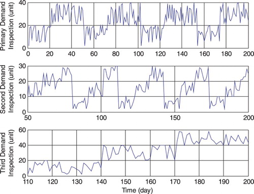
The simulation times are divided into three parts of different long (medium)-term demands. These demands and their beginning time are detected by the inspection unit that is located in the retailer echelon. Also, the penalty of input rate applied in performance index Equation (5) decreases and suppresses deviations of considered values and increases robustness against uncertainties and switches between demand patterns. The simulation stage is operated for 200 time periods. The demands sensed through the forecasting and inspection units are shown in Figure 3. These inspections can be done by parametric comparison between old and new patterns, or traditional vision based on market experience (information references) and then new long-term demands will be forecasted. As shown, in two disjunction points (form change from demand template number one to number two on the 50th day and form change from demand template number two to number three on the 110th day), the patterns are changed and in these time periods, control procedures should be updated according to the defined method described in Equation (5) and Figure 1.

Figure 3. The demand patterns changed in three time stages and inspected by an inspection unit.

In the available case study, each node can be solved independently and share their information with upstream neighbours. The nodes can be simulated under different parameters such as transportation lags, constraints, receding and control horizons, and sharing methods, but in the existing simulations, the parameters of each echelon are the same.

Regarding Figure 2 and the defined structure, until the transition stage between production and distribution (warehouse to distributor), there is a complete symmetric and homogeneous building and order, and delivery communications of the warehouse echelon are symmetric in sequence. Forecasted customer demands are pleaded with retailer nodes as average and equal values and then consequent orders are requested from distributors through retailer nodes, and this procedure is continued as ordering to plant unit by warehouses. This structure can be very useful in one product food industries which some cooperator companies share their sales to supply and to make a special supply chain and to satisfy defined customer demand in a region such as a province or a city (food supply chain in large scales and regions needs more complicate communication and asymmetric). The sharing is because of the large value of the total order that a manufacturer cannot promise to comply to, and hence is compelled to divide the production and distribution and stocking commitments as equal or defined values for satisfying middle nodes and eventually the end customer.

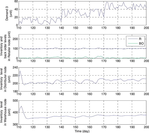
According to Figure 3, the primary demand has an approximate periodicity of 50 time instances, the second demand has an approximate periodicity of 30 time instances, and the third demand has an approximate periodicity of 30 time instances with defined offsets. The complete demand is shown in Figure 4 which shows the deviation steps well. The complete scenario can be explained through this procedure: first of all, in step 1, the problem is completely solved according to the solution stated in the previous part. Step 2 begins by sensing a considerable change in the previous demand pattern (primary demand) on the 50th day and then the inspection unit forces to repeat the solution based on the second forecasted demand and initial values given in the first step. If there is no' change after step 1, the rest of the solution from the first distributed RHC can be continued till the end of the simulation. Also, step 3 is similar to step 2 and is based on the third demand and the change on the 110th day. The simulation results are shown in Figures 5 (based on the primary demand), 6) based on the second demand), and 7 (based on the third demand).

Figure 4. The complete demand.

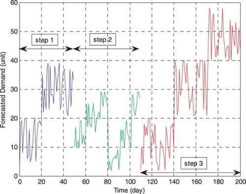
Figure 5. Demand and output variables in the beginning of supply chain decision-making are first confronted with a demand.

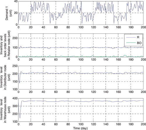
Figure 6. Demand and output variables after confronted with demand 2 at the 50th time instance.

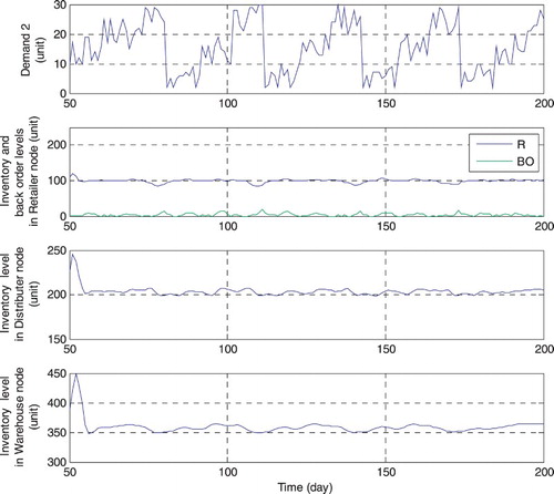
Figure 7. Demand and output variables after confronted with demand 3 at the 110th time instance.

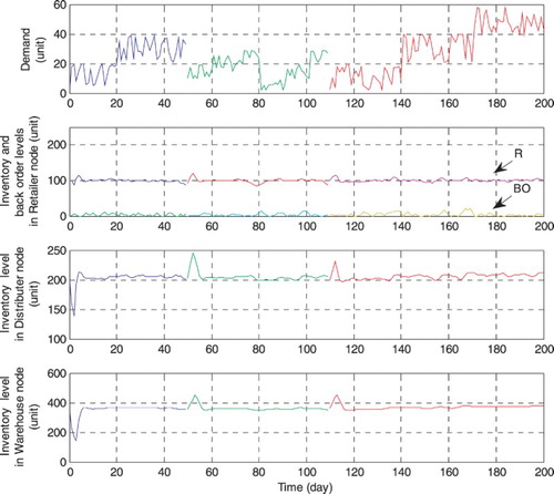
By using the mentioned control procedures, all of the inventories are organized and controlled in limited amplitudes with reasonable deviations in the defined scales very well. Also, the applied RHC is economic and can be settled according to different demand breakpoints by control and prediction horizons and other definable parameters. (Figure 8).

Figure 8. The complete supply chain management plan.

5. Conclusion

In this paper, a distributed control procedure based on RHC and an online inspection unit is utilized. The simulation results show that this method is very impressive in the supply chain field, especially in the field of cooperation and economizing. By this method, as summarized, inventory management for keeping inventories in a band of defined set points, decreasing lead times, increasing robustness, large-scale application, demand inspection, decreasing computational burden by decentralized structure, offline application of distributed control, and customer satisfaction is considered and established. The simulations show that in the case of long-term demands, there is no' need to update control calculations, and predictions permanently; instead, a suitable balance should be made between different influence objects such as sampling times, control and prediction horizons, sharing methods, acceptable delivery time and inventory levels, and back orders.

Disclosure statement

No potential conflict of interest was reported by the authors.

References

- Beamon, B. (1998). Supply chain design and analysis: models and methods. International Journal of Production Economics, 55, 281–294. doi: 10.1016/S0925-5273(98)00079-6
- Camacho, E., & Bordons, C. (2004). Model predictive control (p. 13). Springer.
- Chopra, S., & Meindl, P. (2004). Supply chain management strategy, planning and operations (p. 58). NJ: Pearson Hall Press.
- Dunbar, W., & Desa, S. (2007). Distributed model predictive control for dynamic supply chain management. In R. Findeisen, F. Allgöwer, & L. T. Biegler (Eds.), Assessment and future directions of nonlinear model predictive control (Vol. 358, pp 607–615). Springer.
- Findeisen, R., Allgöwer, F., & Biegler, L. (2011). Assessment and future directions of nonlinear model predictive control. Springer.
- Mastragostino, R., Patel, S., & Swartz, C. (2014). Robust decision making for hybrid process supply chain systems via model predictive control. Computers & Chemical Engineering, 62, 37–55. doi: 10.1016/j.compchemeng.2013.10.019
- Miranbeigi, M., Moshiri, B., & Rahimi-Kian, A. (2014). Decentralized manufacturing management by a multi-agent optimal control method. Transactions of the Institute of Measurement and Control, 36(8), 935–945. doi: 10.1177/0142331214525799
- Miranbeigi, M., Moshiri, B., Rahimi-Kian, A., & Razmi, J. (2015). Demand satisfaction in supply chain management system using a full online optimal control method. The International Journal of Advanced Manufacturing Technology, 77(5), 935–945.
- Perea, E., Grossmann, I., Ydstie, E., & Tahmassebi, T. (2007). Dynamic modeling and classical control theory for supply chain management. Computers and Chemical Engineering, 24, 1143–1149. doi: 10.1016/S0098-1354(00)00495-6
- Sarimveis, H., Patrinos, P., Tarantilis, D., & Kiranoudis, T. (2008). Dynamic modeling and control of supply chain systems: A review. Computers & Operations Research, 35, 3530–3561. doi: 10.1016/j.cor.2007.01.017
- Seferlis, P., & Giannelos, N. (2004). A two-layered optimization-based control strategy for multi-echelon supply chain networks. Computers and Chemical Engineering, 28, 799–809. doi: 10.1016/j.compchemeng.2004.02.022
- Sterman, J. (2002). Business dynamics systems thinking and modelling in a complex world (p. 113). Mcgraw Hill Press.
- Subramanian, K., Rawlings, J. B., & Maravelias, C. (2014). Economic model predictive control for inventory management in supply chains. Computers & Chemical Engineering, 64, 71–80. doi: 10.1016/j.compchemeng.2014.01.003
- Wang, W., & Rivera, R. (2005). A novel model predictive control algorithm for supply chain management in semiconductor manufacturing. Proceedings of the American control conference (Vol. 1, pp. 208–213).