Gradient-based step response identification of overdamped processes with time delay

Abstract

In this paper, a step response identification method is proposed for overdamped industrial processes with time delay from sampled data by developing a gradient searching approach to minimize the output prediction error. Based on establishing a least-squares fitting of the time domain expression of a low-order process model, i.e. first-order-plus-dead-time (FOPDT) or second-order-plus-dead-time (SOPDT), with respect to a step change, the rational model parameters together with the delay parameter can be simultaneously estimated, while the computation effort can be significantly reduced compared to the existing step identification methods based on using the time integral approach for model fitting. Both cases of repetitive poles and distinct poles are considered for the identification of an SOPDT model, along with a guideline for a suitable choice of the model structure for practical applications. The convergence and accuracy of the proposed algorithms are analysed with a strict proof. Four illustrative examples from recent references are used to show the effectiveness of the proposed method.

Keywords:

• step response identification
• overdamped process
• time delay
• second-order-plus-dead-time model
• gradient searching

1. Introduction

For control-oriented model identification in industrial engineering applications, step response tests have been widely used for identifying a transfer function model between the process input and output, owing to its implemental simplicity and economy. In the past decades, the identification of process models with time delay has received increasing attention in view of the fact that time delay is usually involved with industrial processes and system operations (Liu, Wang, & Huang, 2013). Although linear model identification methods have been extensively explored by Rake (1980) and Richard (2003), the extension to identifying a transfer function model with time delay is not straightforward and could become very difficult due to the identification nonlinearity introduced by time delay (Ljung, 1999).

Early references (Gawthrop & Nihtilä, 1985) proposed the approximation of time delay by using Padé approximation and Laguerre expansion, resulting in a higher order rational transfer function model that contains more parameters to be estimated and may cause unacceptable fitting error when the process response has a long time delay. By fitting a few representative points in the transient output response to a step change, Rangaiah and Krishnaswamy (1996) and Huang, Lee, and Chen (2001) reported alternative identification methods for obtaining a first-order-plus-dead-time (FOPDT) or second-order-plus-dead-time (SOPDT) model. Furthermore, based on numerical integral to the time domain expression of step response, Bi et al. (1999) proposed a time integral method for the identification of an FOPDT model, and it has been extended to identify a th order process model by introducing -fold multiple integrals in the lecture, e.g. Wang, Guo, and Zhang (2001) and Wang and Zhang (2001). To cope with load disturbance or nonzero initial conditions, modified step response tests were proposed by Wang et al. (2008), Hwang and Lai (2004) and Wang, Liu, and Hang (2005) to develop robust identification algorithms. Liu, Wang, Huang, and Hang (2007) suggested the use of multiple piecewise step tests to establish LS fitting conditions. In contrast, another robust identification algorithm, proposed by Liu and Gao (2008), was developed for obtaining a low-order transfer function model with time delay by using transient system response data from both adding and removing the step change. The idea was further extended to identify the dynamics of inherent-type load disturbance by Liu, Zhou, Yang, and Gao (2010). Note that these multiple-integral-based identification methods can give good accuracy and robustness in comparison with previous methods, but the computation load is relatively high and the use of multiple time integrals for parameter estimation may be sensitive to the test data length. To avoid the use of multiple time integrals for model identification, Ahmed, Huang, and Shah (2006, 2007) developed an iterative identification method based on using a linear filter. By comparison, a frequency domain step identification method was proposed by Liu and Gao (2010) to relieve the computation effort by introducing a damping factor to the step response for the computation of the Laplace transform.

For the identification of time delay systems, adaptive identification methods for iteratively estimating the linear model parameters and the delay parameter were proposed in the references, e.g. Orlov, Belkoura, Richard, and Dambrine (2003), Ren, Rad, Chen, and Lo (2005), and Na, Ren, and Xia (2014), obtaining good convergence against measurement noise. A generalized expectation–maximization algorithm was proposed for robust global identification of linear parameter-varying systems with fixed input delay (Yang, Lu, & Yan, 2015). For identifying a canonical state space model with state delay, a recursive least-squares parameter identification algorithm was presented by Gu, Ding, and Li (2014) based on using a state filter. To tackle the identification nonlinearity arising from the time delay, a few numerical optimization methods were developed for estimating all the linear model parameters and the delay parameter, e.g. hierarchical identification strategies (Chen, Garnier, & Gilson, 2015; Previdi & Lovera, 2004; Yang, Iemura, Kanae, & Wada, 2007), Gradient searching algorithm (Ding, Liu, & Chu, 2013), Newton iteration approach (Ji, Xu, Xiong, & Chen, 2015), and the Levenberg–Marquardt optimization method (Sung & Lee, 2001; Baysse, Carrillo, & Habbadi, 2011). Note that these numerical optimization methods were developed based on using persistent excitation tests such as the pseudo-random binary sequence (PRBS), and thus are not suitable for step response tests as preferred in many industrial applications.

In this paper, model identification for overdamped industrial processes with time delay is studied to facilitate model-based control design for such a process in industrial applications. A gradient-based identification method is proposed which can simultaneously identify the linear model parameters together with the delay parameter from the step response data. Based on the time domain expression of the process transfer function model with respect to a step change of the input, a modified Gauss–Newton iteration algorithm for parameter estimation is established with computation efficiency for minimizing the output prediction error. Owing to the use of a step test, it is verified that the cost function of prediction error becomes convex with respect to all the model parameters, such that global convergence can be guaranteed. Moreover, no time integral is required for computation, significantly reducing the computation effort compared with recently developed step response identification methods based on using the time integral approach. For clarity, the paper is organized as follows. Section 2 presents the overdamped process models to be identified. The corresponding identification methods are detailed in Section 3. The convergence of the proposed method is analysed in Section 4, together with some guidelines for the choice of a suitable model structure. Four numerical examples are shown in Section 5 to demonstrate the effectiveness of the proposed identification method. Finally, some conclusions are drawn in Section 6.

2. Overdamped process model

For industrial overdamped processes, e.g. multi-component blending reactors and fermentation tanks, a low-order model of FOPDT or SOPDT is widely used for control system design and tuning (Seborg, Mellichamp, Edgar, & Doyle, 2010). Without loss of generality, two model forms are studied in this paper, one has a single or repetitive poles, (1) and the other has two distinct poles, (2) where denotes the process static gain, is the process time delay, , and are time constants, and is the number of repetitive poles or the model order.

It should be noted that higher-order overdamped processes can be effectively described by the above models (Seborg et al., 2010; Liu & Gao, 2012).

Under a step test, the input excitation with a magnitude of can be described by (3)

Correspondingly, the output response subject to measurement noise may be written as (4) where denotes the true output, and is usually assumed to be a white noise with zero mean.

Generally, the process static gain, , can be directly computed from (5) where is obtained by averaging 20–30 measured output values after the process response moves into a steady state in a step test.

Define the model prediction error and cost function, respectively, as (6) (7) where , denotes the estimation of unknown parameters, is the output prediction, denotes the collected data length, and () are the sampled instant which should be chosen such as . Denote by a column vector all the unknown parameters to be identified.

Hence, the identification objective is to estimate the unknown parameters in Equation (1) or Equation (2) from the input–output observations (), satisfying (8)

3. Proposed identification algorithms

Two gradient-based identification algorithms are developed to identify overdamped process models in Equations (1) and (2), as detailed in the following two subsections.

3.1. Time delay model with single or repetitive poles

Letting in Equation (1) leads to an FOPDT model. Correspondingly, the time domain step response under zero initial conditions can be expressed by (9) where , and the static gain is computed by Equation (5).

Similarly, for the case of in Equation (1), the time domain step response can be derived as (10)

For brevity, the identification procedure is detailed for the case of , which can be simply extended to a case of .

To estimate the unknown model parameters, we let (11)

The prediction error can be computed from Equation (9) as (12)

To minimize the cost function in Equation (7), we take the first-order derivative for Equation (12) with respect to and , respectively, obtaining (13) (14)

The Jacobian matrix of Equation (12) is defined by (15)

Denote (16)

The gradient matrix of with respect to is therefore defined by (17)

The corresponding Hessian matrix is formulated by (18)

Hence, the parameter vector can be estimated using a Gauss–Newton iteration approach, i.e. (19) where and can be computed from Equations (17) and (18) in terms of estimated from the previous iteration step. The initial estimation of may be taken as a vector composed of small positive real numbers while the delay parameter may be taken roughly about the minimal output response delay as can be observed from a step test.

It is well known that the standard Gauss–Newton iteration method may give a very slow convergence rate in the initial stage of the iterative process for parameter estimation, causing a considerable computation effort. To overcome the deficiency, we propose the use of an adaptive step length for iteration based on the Armijo line searching strategy (see, e.g. Wright & Nocedal, 1999), i.e. (20) where denotes the searching direction, and are generally required for computation, and is the minimal nonnegative integer satisfying (20).

To accomplish the identification objective in Equation (8) using less computation effort, it is suggested to take the searching step, (21) (22) and for the implementation of (20). Note that is step-wise varying with respect to the prediction error. Initially, there is likely to be a larger difference between and , which may turn out to be a larger value of from Equation (21) that results in a larger step for searching and thus expedites the convergence rate (i.e. reducing the number of external loop iteration relating to the searching step). The lower limit in Equation (22) is set to avoid an over large value of that may cause severe increment of the iteration number of the internal loop iteration for determining . As the iteration goes on, and gradually approach the identity, resulting in that guarantees the searching step not very small to maintain the convergence rate. Owing to the fact that (), there follows which satisfies the general requirement of the Armijo line searching method.

Another issue involved with the Gauss–Newton iteration method is that a suitable initial value is required for iteration, since a local minimum of solution might be turned out for an arbitrary choice of the initial value. To address the issue, numerical simulations are explored to study the relationship between and the model parameters based on using different input excitations for identification. Consider a second-order process with time delay described by where and . The input excitation is taken as a unity step change or a PRBS sequence with the variance of respectively, for comparison. The number of measured output data is and the sampling period is (s). 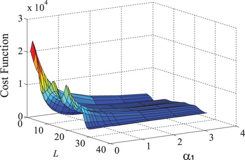Assuming that the searching ranges of the model parameters are and , the corresponding between the process response and model response are plotted in Figures 1 and 2 to the input excitations of the step change and PRBS sequence, respectively. It is seen from Figure 1 that there is a unique global minimum, owing to the fact that a step change mainly includes low-frequency components that provoke the output response basically in the low-frequency range. This indicates that using a step test for model identification is not sensitive to the initial choice of model parameters for iteration. In contrast, it is seen from Figure 2 that there are multiple local minimums, which implies that different choices of initial model parameters for iteration will turn out different identification results converging to any local minimums of .

Figure 1. Plot of the identification cost function under a step test.

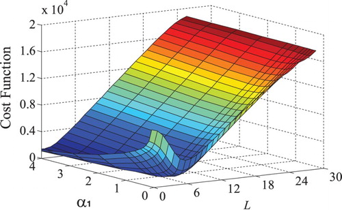
Figure 2. Plot of the identification cost function under a PRBS excitation.

Based on the above analysis, it is suggested to take the initial values of all the model parameters in Equation (1) or Equation (2) as a small positive real number for iteration. To improve the convergence rate, the delay parameter may be taken roughly about the minimum of the possible range as can be observed from a step test.

Hence, the above algorithm named Algorithm I for obtaining a time delay model with a single or repetitive poles can be summarized as

1. Collect the input–output observations () from a step test, and compute the process static gain in terms of Equation (5).

2. Take the initial estimation of as a vector composed of small positive real numbers while the delay parameter may be taken roughly about the minimal output response delay as can be observed from a step test.

3. Compute the prediction error and using Equations (12) and (7).

4. Determine the searching direction by computing the gradient matrix in Equation (17) and the Hessian matrix in Equation (18).

5. Take the searching step in terms of Equation (22).

6. Update , where , and is the minimal nonnegative integer that satisfies (20) with the choice of Equation (22).

7. End the algorithm if the fitting condition, , is satisfied, where is a user specified fitting threshold, or the maximum iteration number is attained. Otherwise, let and go to step (iii).

3.2. Second-order time delay model with distinct poles

The time domain step response of the process model in Equation (2) is in the form of (23) where , , and .

Denote the parameter vector for estimation, (24)

The prediction error can be computed based on the static gain estimated by Equation (5) as (25)

To minimize the cost function in Equation (7), we take the first-order derivative for Equation (25) with respect to , and , respectively, obtaining (26)

Correspondingly, the gradient matrix of and the Hessian matrix can be computed in terms of Equations (17) and (18), respectively.

Hence, an identification algorithm named Algorithm II for obtaining an SOPDT model with distinct poles can be summarized as

1. Collect the input–output observations () from a step test, and compute the process static gain in terms of Equation (5).

2. Take the initial estimation of as a vector composed of small positive real numbers while the delay parameter may be taken roughly about the minimal output response delay as can be observed from a step test.

3. Compute the prediction error and cost function using Equations (25) and (7).

4. Determine the searching direction by computing the gradient matrix in Equation (17) and the Hessian matrix in Equation (18).

5. Take the searching step in terms of Equation (22).

6. Update , where , and is the minimal nonnegative integer that satisfies (20) with the choice of Equation (22).

7. End the algorithm if the fitting condition, , is satisfied, where is a user specified fitting threshold, or the maximum iteration number is attained. Otherwise, let and go to step (iii).

Remark 1

It can be seen from the above algorithms that the identification procedure is relatively independent of the time length of the step response and use no time integral for computation, significantly reducing the computation effort compared with the recently developed step identification methods based on using single or multiple time integrals to the step response data (Ahmed, Huang, & Shah, 2008; Liu et al., 2007, 2010).

4. Analysis on consistency estimation

For practical application in the presence of measurement noise, it should be clarified if consistent estimation could be guaranteed by the proposed method. To address this issue, the following proposition is given accordingly.

Proposition 1

Assuming that is differentiable with respect to in a neighbourhood of the bounded level set , and the Jacobian matrix in Equation (16) is full row rank together with the positive-definite Hessian matrix in (18), both Algorithms I and II guarantee uniform convergence satisfying (27) where .

Proof

By assuming is differentiable with respect to in the bounded set , there follows for some positive constants and that (28) (29)

where denotes the matrix 2-norm.

It can be verified that there exists a constant such that (30)

Owing to that is full column rank, there stands for a sufficient large constant, , such that (31)

Denote by the intersection angle between the negative gradient direction, , and the Gauss–Newton searching direction, . It can be derived using Equations (30) and (31) that (32)

From the Armijo condition in (20), we obtain (33) where .

Summing (33) over all indices of yields (34)

Considering that is a bounded value, we ensure that is finite for all , and therefore take the limit to both sides of (34), obtaining (35) which implies that (36) With , is positive definite, and , it follows that

This completes the proof.

Note that the convergence result shown in Equation (27) indicates that the cost function converges to a steady value when , that is to say, the estimated model parameters converge to the true values for perfect model match with the plant, leading to .

According to Proposition 1, the proposed algorithm guarantees convergence in the presence of measurement noise, owing to the fact that (37) and (38)

Therefore, the iterative process of the proposed algorithm will not be affected by the measurement noise, guaranteeing good robustness for convergence.

Note that it is often encountered in practical applications that the true model structure of the process to be identified cannot be known exactly. It is desirable to determine an optimal model structure for representing the process dynamic response characteristics from a step test. The following hypothesis testing condition, which was introduced in Liu and Gao (2010), can be taken for the choice of optimal model order, (39) where and denote, respectively, the measured process output and the model output to the step change, denotes the current model order and a higher order to be verified.

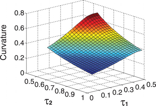
It can be seen from Equation (39) that a higher model order should be accepted only if the output prediction error is larger than one-tenth of that of the current model with . To determine if an SOPDT model with repetitive poles or distinct poles should be chosen, we define the curvature (see, e.g. Rynne & Youngson, 2000) of such a model response to a step change by (40) where and denote the first-order and second-order derivatives, respectively. The maximal curvature for the normalized ranges of , and in these two models is plotted in Figures 3 and 4, respectively. It is seen from Figure 3 that an evidently larger curvature occurs for an SOPDT model with repetitive poles compared with Figure 4 for an SOPDT model with distinct poles. Therefore, it is suggested to take an SOPDT model with repetitive poles if the process response to a step change has an obviously larger curvature.

Figure 3. The maximal curvature of an SOPDT model with repetitive poles.

Figure 4. The maximal curvature of an SOPDT model with distinct poles.

5. Illustration

Four examples from the recent literatures are studied here to illustrate the performance of the proposed method. Examples 1–3 are given to show good accuracy of the proposed algorithms for identifying low-order processes in terms of the exact model structures, together with measurement noise tests to demonstrate identification robustness. Example 4 is used to show the effectiveness of the proposed algorithm for identification of higher order processes. In the following examples, the measurement noise level is evaluated in terms of the noise-to-signal ratio, (41)

The following time domain fitting criterion is used to assess identification accuracy, (42) where is the actual process output and is the response of the estimated model.

The parameter estimation error is assessed by the following criterion: (43) where is an estimation of the true parameter vector .

Example 1

Consider the first-order inertial system with time delay studied by Bi et al. (1999),

Based on a unity step response test, Bi et al. (1999) gave a FOPDT model, , by using a time domain integral of the output response for LS fitting. For illustration, the same step test is performed with the sampling interval ( s) and the sampling time (s). According to the proposed guideline for choosing the initial values for iteration, is taken to apply the proposed Algorithm I, resulting in the exact model parameters based on any data length longer than the transient step response time.

Then assume that the process output measurement is corrupted by a Gaussian white noise with NSR = 10% and NSR = 20%, respectively. The estimation results are listed in Table 1 together with the iteration results. It can be seen from Table 1 that the proposed algorithm converges quickly regardless of poor initial estimation for iteration. Moreover, 100 Monte Carlo tests are conducted under a variety of random measurement noise level (NSR = 10%, 20%) for using the proposed algorithm. Table 2 lists the simulation results where the internal loop indicates the iteration number for determining in (20), and the external loop indicates the iteration number of searching step for converging to the optimal estimation. It is seen from Table 2 that the proposed algorithm guarantees a fast convergent speed and maintain good robustness against measurement noise. The computation load of the proposed method is listed in Table 3 in comparison with that of the time integral method given by Bi et al. (1999), where denotes the number of sampled data for identification and is the number of iterative steps. Owing to the fact that is much larger than , the computation load is significantly reduced by the proposed method.

Table 1. Identification results under different noise levels for Example 1.

NSR	Iterative step			ERR (%)
10%	1	77.3769	−90.85	8446.80
	5	30.8218	−49.83	4167.30
	10	10.5482	−13.45	1224.50
	20	1.2032	0.91	15.73
	30	0.9816	0.99	1.35
20%	1	77.8236	−91.11	8481.00
	5	32.1390	−52.4817	4376.00
	10	12.1918	−17.06	1502.49
	20	1.5376	0.72	42.97
	30	0.9638	0.99	2.67
	35	0.9633	0.99	2.70
True value		1	1	0

Table 2. Averaged iteration numbers under 100 Monte Carlo tests for Example 1.

NSR	External loop	Internal loop	Success ratio
10%	48	81	100
20%	49	84	99

Table 3. Comparison of the computation load for Example 1.

Methods	Addition	Multiplication
Proposed
Bi et al. (1999)

Example 2

Consider a second-order process with repetitive poles studied by Liu et al. (2007), (44)

A square wave with an amplitude 1 and a period (s) was adopted as the input excitation in lecture Liu et al. (2007), obtaining an estimated model,

For illustration, a unity step response test is used in the proposed method where the sampling period is taken as (s) and the overall sampling time is (s).

To test identification robustness against measurement noise, assume that the noise level is NSR = 10% in the step test. By performing 100 Monte Carlo tests in terms of randomly varying the ‘seed’ of the noise generator, the proposed algorithm gives which indicates improved identification accuracy.

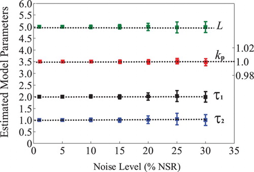
To demonstrate consistent estimation against measurement noise, the identification results for different noise levels (NSR = 5%, 10%, 15%, 20%, 25%, 30%) are shown in Figure 5, where the result for each model parameter to a given noise level is shown as a vertical linear segment along with the sample standard deviation in parentheses for 100 Monte Carlo tests. The square solid point in each linear segment denotes the mean of 100 identification results, and the upper and lower bars correspond to the maximum and the minimum of parameter estimation, respectively. It is seen that good identification accuracy and consistent estimation are obtained against different noise levels. Moreover, it can be easily verified that, given a measurement noise level, the sample standard deviation of the proposed estimation error is much smaller than that of the measurement noise.

Figure 5. The results of 100 Monte Carlo Tests for Example 2 against measurement noise.

Figure 6 shows the estimation results of the proposed method for different lengths (N) of data in a range from 165 to 8000 with . For data collection with respect to different data lengths, the sampling interval is taken as . It is seen that good identification accuracy can be obtained for a wide range of data lengths and the estimation results become better as the number of data points increases or the sampling interval decreases. Moreover, the computation load is listed in Table 4 in comparison with that of Liu et al (2007) based on using the time integral approach, indicating that the computation effort is significantly reduced by the proposed method.

Figure 6. Parameter estimation with respect to data length for Example 2.

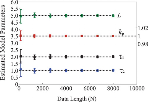
Table 4. Comparison of the computation load for Example 2.

Methods	Addition	Multiplication
Proposed
Liu et al. (2007)

Example 3

Consider a second-order process with distinct poles studied by Wang, Liu, Hang, and Tang (2006), (45)

By performing a step test with a sampling period (s) and the sampling time (s), the proposed Algorithm II gives an exact estimation of the process model based on any data length longer than the transient step response time.

Then assume that the process output measurement is corrupted by a white noise causing . The iteration process of the proposed Algorithm II is listed in Table 5 with an initial choice of , indicating good convergence rate and identification accuracy.

Table 5. Parameter estimation results for Example 3.

Iterative step				ERR (%)
1	10.0000	3.3333	0.10	103.78
10	7.0847	0.6124	10.83	98.21
20	3.6830	0.6836	8.36	60.10
30	5.0930	0.5387	5.68	18.68
40	4.9999	1.0274	4.57	1.20
True value	5	1	4.5	0

Example 4

Consider the fifth-order system with time delay studied by Wang et al. (2001)

Based on a step test, Wang et al. (2001) derived an SOPDT model, , corresponding to the mean-squared output fitting error, . For comparison, the same step test is performed for the sampling time (s) with the sampling interval (s). The proposed Algorithm II gives an SOPDT model, , corresponding to .

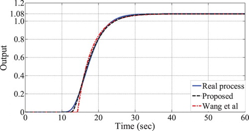
Then assume that the output measurement noise level is NSR=10%, the proposed method gives , corresponding to , compared with that proposed by Wang et al. (2001) , corresponding to . The step responses of these models are shown in Figure 7, well demonstrating good fitting of the proposed method.

Figure 7. Step response fitting for Example 4.

6. Conclusions

A step response identification method has been proposed for overdamped industrial processes with time delay, along with a proof on the convergence and consistency in the presence of measurement noise. By developing a gradient-based searching approach to minimizing the output prediction error, the linear model parameters together with the delay parameter can be simultaneously identified from the time domain expression of a low-order model response to a step change, specifically for the identification of an FOPDT or SOPDT model. A guideline of model structure selection has been given for identifying an SOPDT model with repetitive poles or distinct poles. The computation effort can be significantly reduced compared to recently developed step response identification methods (e.g. Ahmed et al., 2008; Liu et al., 2007, 2010) based on using the time integral to step response data and, moreover, the proposed algorithms are not sensitive to the data length for model identification, therefore facilitating practical applications. Four illustration examples from the literature have well demonstrated that the effectiveness and accuracy of the proposed identification algorithms. It should be noted that the proposed method cannot be applied to an underdamped process with complex poles that hinder the use of a gradient searching strategy for minimizing the output prediction error, which will be studied in our future work.

Additional information

Funding

This work is supported in part by the National Thousand Talents Program of China, NSF China Grants 61473054, and the Fundamental Research Funds for the Central Universities of China.

References

- Ahmed, S., Huang, B., & Shah, S. L. (2006). Parameter and delay estimation of continuous-time models using a linear filter. Journal of Process Control, 16(4), 323–331. doi: 10.1016/j.jprocont.2005.07.003
- Ahmed, S., Huang, B., & Shah, S. L. (2007). Novel identification method from step response. Control Engineering Practice, 15(5), 545–556. doi: 10.1016/j.conengprac.2006.10.005
- Ahmed, S., Huang, B., & Shah, S. L. (2008). Identification from step responses with transient initial conditions. Journal of Process Control, 18(2), 121–130. doi: 10.1016/j.jprocont.2007.07.009
- Baysse, A., Carrillo, F. J., & Habbadi, A. (2011). Time domain identification of continuous-time systems with time delay using output error method from sampled data. The 18th IFAC World Congress, Milano, Italy.
- Bi, Q., Cai, W. J., Lee, E. L., Wang, Q. G., Hang, C. C., & Zhang, Y. (1999). Robust identification of first-order plus dead-time model from step response. Control Engineering Practice, 7(1), 71–77. doi: 10.1016/S0967-0661(98)00166-X
- Chen, F., Garnier, H., & Gilson, M. (2015). Robust identification of continuous-time models with arbitrary time-delay from irregularly sampled data. Journal of Process Control, 25, 19–27. doi: 10.1016/j.jprocont.2014.10.003
- Ding, F., Liu, X., & Chu, J. (2013). Gradient-based and least-squares-based iterative algorithms for Hammerstein systems using the hierarchical identification principle. IET Control Theory & Applications, 7(2), 176–184. doi: 10.1049/iet-cta.2012.0313
- Gawthrop, P. J., & Nihtilä, M. T. (1985). Identification of time delays using a polynomial identification method. Systems & Control Letters, 5(4), 267–271. doi: 10.1016/0167-6911(85)90020-9
- Gu, Y., Ding, F., & Li, J. (2014). State filtering and parameter estimation for linear systems with d-step state-delay. IET Signal Processing, 8(6), 639–646. doi: 10.1049/iet-spr.2013.0076
- Huang, H. P., Lee, M. W., & Chen, C. L. (2001). A system of procedures for identification of simple models using transient step response. Industrial & Engineering Chemistry Research, 40(8), 1903–1915. doi: 10.1021/ie0005001
- Hwang, S. H., & Lai, S. T. (2004). Use of two-stage least-squares algorithms for identification of continuous systems with time delay based on pulse responses. Automatica, 40(9), 1561–1568. doi: 10.1016/j.automatica.2004.03.017
- Ji, K., Xu, L., Xiong, W., & Chen, L. (2015). Newton iterative algorithm based modeling and proportional derivative controller design for second-order systems. Journal of Applied Mathematics and Computing, 49(1), 557–572. doi: 10.1007/s12190-014-0853-7
- Liu, M., Wang, Q. G., Huang, B., & Hang, C. C. (2007). Improved identification of continuous-time delay processes from piecewise step tests. Journal of Process Control, 17(1), 51–57. doi: 10.1016/j.jprocont.2006.08.002
- Liu, T., & Gao, F. (2008). Robust step-like identification of low-order process model under nonzero initial conditions and disturbance. IEEE Transactions on Automatic Control, 53(11), 2690–2695. doi: 10.1109/TAC.2008.2007172
- Liu, T., & Gao, F. (2010). A frequency domain step response identification method for continuous-time processes with time delay. Journal of Process Control, 20(7), 800–809. doi: 10.1016/j.jprocont.2010.04.007
- Liu, T., & Gao, F. (2012). Industrial process identification and control design: Step-test and Relay-experiment-based Methods. London: Springer.
- Liu, T., Wang, Q. G., & Huang, H. P. (2013). A tutorial review on process identification from step or relay feedback test. Journal of Process Control, 23(10), 1597–1623. doi: 10.1016/j.jprocont.2013.08.003
- Liu, T., Zhou, F., Yang, Y., & Gao, F. (2010). Step response identification under inherent-type load disturbance with application to injection molding. Industrial & Engineering Chemistry Research, 49(22), 11572–11581. doi: 10.1021/ie1015427
- Ljung, L. (1999). System identification: Theory for the user. 2nd ed. Englewood Cliff, NJ: Prentice-Hall.
- Na, J., Ren, X. M., & Xia, Y. (2014). Adaptive parameter identification of linear SISO systems with unknown time-delay. Systems & Control Letters, 66, 43–50. doi: 10.1016/j.sysconle.2014.01.005
- Orlov, Y., Belkoura, L., Richard, J. P., & Dambrine, M. (2003). Adaptive identification of linear time- delay systems. International Journal of Robust and Nonlinear Control, 13(9), 857–872. doi: 10.1002/rnc.850
- Previdi, F., & Lovera, M. (2004). Identification of non-linear parametrically varying models using separable least squares. International Journal of Control, 77(16), 1382–1392. doi: 10.1080/0020717041233318863
- Rake, H. (1980). Step response and frequency response methods. Automatica, 16, 519–526. doi: 10.1016/0005-1098(80)90075-8
- Rangaiah, G. P., & Krishnaswamy, P. R. (1996). Estimating second-order dead time parameters from underdamped process transients. Chemical Engineering Science, 51(7), 1149–1155. doi: 10.1016/S0009-2509(96)80013-3
- Ren, X. M., Rad, A. B., Chen, P. T., & Lo, W. L. (2005). Online identification of continuous-time systems with unknown time delay. IEEE Transactions on Automatic Control, 50(9), 1418–1422. doi: 10.1109/TAC.2005.854640
- Richard, J. P. (2003). Time-delay systems: an overview of some recent advances and open problems. Automatica, 39(10), 1667–1694. doi: 10.1016/S0005-1098(03)00167-5
- Rynne, B. P., & Youngson, M. A. (2000). Linear functional analysis. London: Springer.
- Seborg, D. E., Mellichamp, D. A., Edgar, T. F., & Doyle, III F. J. (2010). Process dynamics and control. 3rd ed. Hoboken, NJ: John Wiley & Sons.
- Sung, S. W., & Lee, I. B. (2001). Prediction error identification method for continuous-time processes with time delay. Industrial & Engineering Chemistry Research, 40(24), 5743–5751. doi: 10.1021/ie0100636
- Wang, Q. G., Guo, X., & Zhang, Y. (2001). Direct identification of continuous time delay systems from step responses. Journal of Process Control, 11(5), 531–542. doi: 10.1016/S0959-1524(00)00031-7
- Wang, Q. G., Liu, M., & Hang, C. C. (2005). Simplified identification of time-delay systems with nonzero initial conditions from pulse tests. Industrial & Engineering Chemistry Research, 44(19), 7591–7595. doi: 10.1021/ie050104o
- Wang, Q. G., Liu, M., Hang, C. C., & Tang, W. (2006). Robust process identification from relay tests in the presence of nonzero initial conditions and disturbance. Industrial & Engineering Chemistry Research, 45(12), 4063–4070. doi: 10.1021/ie051317g
- Wang, Q. G., Liu, M., Hang, C. C., Zhang, Y., Zhang, Y., & Zheng, W. X. (2008). Integral identification of continuous-time delay systems in the presence of unknown initial conditions and disturbances from step tests. Industrial & Engineering Chemistry Research, 47(14), 4929–4936. doi: 10.1021/ie071532s
- Wang, Q. G., & Zhang, Y. (2001). Robust identification of continuous systems with dead-time from step responses. Automatica, 37(3), 377–390. doi: 10.1016/S0005-1098(00)00177-1
- Wright, S. J., & Nocedal, J. (1999). Numerical optimization. New York, NY: Springer.
- Yang, X., Lu, Y., & Yan, Z. (2015). Robust global identification of linear parameter varying systems with generalised expectation–maximisation algorithm. IET Control Theory & Applications, 9(7), 1103–1110. doi: 10.1049/iet-cta.2014.0694
- Yang, Z. J., Iemura, H., Kanae, S., & Wada, K. (2007). Identification of continuous-time systems with multiple unknown time delays by global nonlinear least-squares and instrumental variable methods. Automatica, 43(7), 1257–1264. doi: 10.1016/j.automatica.2006.12.026