Fuzzy fault-tolerant-predictive control for a class of nonlinear uncertain systems

ABSTRACT

In this paper, a fault-tolerant fuzzy model-predictive control with the integral action method for a class of nonlinear uncertain systems is proposed. Nonlinear uncertain systems subject to actuators and/or sensors faults are represented by the Takagi–Sugeno (T-S) fuzzy model. The objective is to design a stable, robust and efficient fault-tolerant controller based on a T-S fuzzy observer with measurable premise variables. The proposed T-S fuzzy observer estimates state vector and faults. Based on Lyapunov theory, the trajectory tracking performances and the closed-loop system stability are analysed. The gains of the fuzzy observer and the pre-stabilized control law are obtained by solving linear matrix inequalities. Simulation results illustrate the robustness of the proposed controller with respect to uncertainties on an academic mathematical system.

KEYWORDS:

• T-S models
• fault and state estimation
• model-predictive control
• nonlinear uncertain systems
• linear matrix inequalities

1. Introduction

In the presence of faults, the fault-tolerant controller (FTC) aims are to conserve the stability and the performances of the nonlinear uncertain system. Nonlinear uncertain systems subject to faults could be represented by T-S fuzzy models. The T-S fuzzy modelling is adopted in this paper to describe the nonlinear system dynamics behaviour. In Takagi and Sugeno (1985), the overall system behaviour is approximated with N submodels around several operational areas. In Tanaka, Ikeda, and Wang (1996), Tanaka, Hori, and Wang (2001), the stability and stabilization of T-S fuzzy models are studied. Formulation of the stability conditions in terms of LMI derived from Lyapunov theory are used. Tanaka, Ikeda, and Wang (1998) studied quadratic stability and they showed that it is difficult to obtain a common Lyapunov matrix satisfying a set of LMIs, as well as the number of submodels increases. In Johansson (1999), Tanaka, Hori, and Wang (2003), authors developed polyquadratic and non-quadratic approaches. Chadli, Aouaouda, Karimi, and Shi (2013) deal with the FTC design based on T-S fuzzy modelling for a vertical takeoff and landing aircraft subject to external disturbances and actuator faults. Aouaouda, Chadli, Khadira, and Bouarara (2012) used descriptor redundancy property and L optimization to attenuate the unknown inputs effect. They have proposed a solution in terms of bilinear matrix inequalities to control a model of the wastewater treatment plant. Estimation and observation techniques of some nonlinear dynamics parameters are required for the FTC design. In Bergsten and Palm (2002), these approaches are extended for observer design applied to state and unknown input estimation. In Aouaouda, Chadli, and Ichalal (2013), the stability and stabilization of T-S fuzzy models subject to faults are studied. The authors proposed an FTC strategy based on T-S fuzzy observer for vehicle lateral dynamics. In our previous works (Ben Hamouda, Bennouna, Ayadi, and Langlois, 2014b,c), fuzzy model-based observer was developed for T-S fuzzy models. The objective is to ensure the convergence of the state estimation errors to zero. The proposed control strategy is based on a combination between parallel distributed compensation (PDC) and model-predictive control (MPC) with the T-S fuzzy approach. MPC solves an optimization to achieve the desired set points and control objectives (Maciejowski, 2002). The feasibility of the optimization problem provides the guarantee of the nominal asymptotic stability (Kale and Chipperfield, 2005). However, the optimization can be infeasible due to faults. This motivates the development of the proposed approach to recover feasibility with respect of constraints imposed on control inputs and system states. In order to point the approaches proposed in Ben Hamouda, Bennouna, Ayadi, and Langlois (2014a), Ben Hamouda et al. (2014b,c), the uncertain case is considered. In Chadli et al. (2013) and Aouaouda et al. (2012), the authors proposed a robust FTC for uncertain and disturbed T-S fuzzy models. The authors synthesized an FTC ensuring trajectory tracking for a nonlinear uncertain system represented by the T-S model. In Kumar Dohare, Singh, and Kumar (2015), it has been observed that MPC shows good performances even in the presence of uncertainties on the BTX (benzene–toluene–o-xylene ) system. The variation of these parameters is for the nominal values of the feed flow rate, feed composition and liquid split factor. In Jamal Alden and Wang (2015), a novel robust control framework based on LMI is proposed for a power-generation system with time delays, model uncertainties and disturbances. In Fekih and Seelem (2015), a proposed approach is designed to maintain vehicle stability, dynamics and manoeuvrability in the event of a faulty steering system. A sensor fusion-based fault detection and identification approach is proposed to accurately detect and identify sensor faults when they occur. A weight adjustment algorithm is considered to ensure accurate detection while providing robustness against parameter variations and uncertainties. The authors proposed a controller which incorporates a linear quadratic regulator (LQR)-based algorithm with afeed-forward gain.

This papers deals with the tracking problem for the uncertain T-S and faulty models. The main contribution of the paper is to propose an LMI formulation to derive the proposed FTC law with respect to uncertainties on the model parameters. The layout of this paper is as follows: in Section 2, a faulty T-S fuzzy uncertain model representation is given. Then in Section 3, fuzzy model-predictive control (FMPC) with integral action method for uncertain nonlinear systems is proposed. Section 4 shows the simulation results. Conclusion is presented in the last section.

2. T-S Fuzzy modelling

2.1. T-S Model representation

Let h and g be two nonlinear functions and the output such that the system state space representationis (1) where stands for the state and denotes the control input. The T-S fuzzy model is based on rules as those of Takagi and Sugeno (1985): IF PREMISE THEN CONSEQUENCE. Premises represent the system nonlinearities and consequences correspond to submodels. The considered T-S fuzzy model is based on an interpolation between N local linear models. Three several methods can be employed to obtain a T-S model, through identification and parameters estimation from experimental data, direct transform of an affine model in the state and linearization around different operating points. Tanaka et al. (1996) obtain a convex polytopic representation by a direct transform of an affine model in the state. This method does not generate an approximation error and has the advantage of reducing the local model number. Polytope is obtained with peaks, where r is the number of premise variables. In Ben Hamouda, Bennouna, Ayadi, and Langlois (2013), a non-stationary linearization method of a class of nonlinear system subject to faults is proposed to obtain a T-S fuzzy model. The fuzzy model obtained is constituted by two sets of sub-linear time invariant (LTI) model representing the lower and upper bounds , as described in Orjuela, Marx, Maquin, and Ragot (2008); Orjuela, Marx, Ragot, and Maquin (2009), Rodrigues, Adam-Medi, Theilliol, and Sauter (2008) and Ichalal, Marx, Maquin, and Ragot (2012). The precise knowledge of the upper and lower bounds is not always possible. In fact, premise variables depend on nonlinearities system. For some systems, the lower and upper bounds are unknown. The influence of this problem is discussed in Nagy (2010) through an example. The T-S fuzzy model obtained is given by the following relation (Tanaka et al., 2001): (2) where , and are constant matrices. The submodel matrices are assumed to be asymptotically stable. θ represents the premise variables vector depending on system states and input and is the ith activation function. determines the activation degree of the ith associated local model, by providing a gradual transition from this model to local model neighbours. These functions satisfy the following properties: (3) The knowledge of the activation functions is fundamental for designing the control law. The choice of the premise variables is based on a set of criteria. In Bergsten and Palm (2002), these criteria are constructed in accordance with stability analysis and/or observability objectives. The structure fuzzy model is described by the weighting functions . Indeed, the ith linear model describes the system dynamics around the ith operating point. Variations of the vector θ are represented by a set of the M^th peak matrices which define the polytope. Under the condition that the matrix M is considered as a matrix of submodels. The following sub-section gives a T-S fuzzy representation of faulty uncertainsystems.

2.2. Faulty uncertain T-S Model

In the faulty case, it is supposed the nonlinear model (2(2) ) can be described by (4) with and where , , and represent, respectively, the faulty state, faulty measured output vectors, the FTC signal and the fault signal vectors. and are, respectively, the actuator fault and the sensor fault matrices and represents the uncertainty matrix with appropriate dimensions. The uncertainty matrix represents a parameters variation equal to for the nominalvalues.

In the next section, a T-S fuzzy controller for uncertain nonlinear systems subject to faults is proposed. The main objective is to tolerate faults while achieving tracking desired trajectory.

3. Fault-tolerant controller design

3.1. Studied MPC-based strategy

For nonlinear systems, there exist some forms of constraints due to physical, economic, safety or performance requirements on system states, control inputs and control rates. The advantage of MPC is the possibility to handle the prediction algorithm with the respect of constraints on the states and inputs. The MPC structure allows FTC to be embedded: constraints can be redefined, internal model and the control objectives can be changed. The desired state of the reference model is subtracted from the measured plant state. The MPC controller has a regulator form. The aim of MPC is to minimize a cost function J to compute the optimal control: (5) where the following constraints are considered: and is the predicted response and is the output desired trajectory. The matrices Q and R weigh the corresponding control errors and control actions. The R matrix helps to keep the control inputs within bounds, making sure that smooth control actions result. and are output and control prediction horizons, respectively. The prediction horizon is chosen bigger than the control horizon. A short control horizon is chosen to make the system more robust to uncertainties. The model defines the internal dynamic model. The controllability condition is required. This condition ensures the feasibility at each step of the MPC optimization solved. Only the first control increment is implemented and the optimization is re-solved at each step.

In the next sub-section, an FTC strategy is proposed to recover feasibility with the respect of control inputs, system state constraints and uncertainty system parameters.

3.2. Structure of the proposed FMPC strategy

The proposed FTC strategy uses a T-S fuzzy observer to estimate system states and to detect faults. The proposed FMPC approach should maintain system output close to the desired trajectories and preserve stability conditions even when the faults occur. In our previous work (Ben Hamouda et al., 2014b,c), the proposed ith control law signal generated in the nominal operating is given by the following: (6) where , are the integral action gain, represents the estimated state, are the N state feedback gains and the ith predicted control input signal calculated by the FTC. is set to zero, after the end of the control horizon. The control law applied becomes (7) Providing further robustness and accuracy is the second feedback aim (Ben Hamouda et al., 2013). This strategy guarantees the nominal closed-loop stability (Afonso and Galvao, 2010). The integral action helps to drive the tracking error to zero. The fault-tolerant controller is shown in the scheme of Figure 1.

Figure 1. The fault-tolerant control strategy based on the faulty uncertain T-S model.

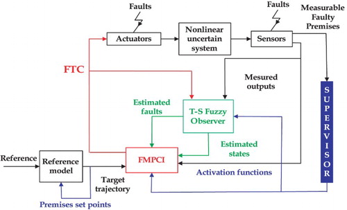
The strategy given in Figure 1 is proposed to determine the control inputs such that:

• the closed-loop system is stable,

• converges asymptotically to the reference state vector even in the presence of faults and uncertainties on the system parameters.

In our previous work (Ben Hamouda et al., 2014b,c), the following FTC strategy based on the interpolation mechanism is proposed: (8) where is the fault estimate vector and is the stabilized predicted control input in the nominal operating given by Equations (5(5) )–(7(7) ). The nominal control represents a combination between the PDC and the MPC with the integral action method. The MPC optimization problem to solve is a quadratic programmable (QP) problem. The activation functions and are defined by (9) where . The FMPC objective is to compute in such a way that the closed-loop system including the state and fault estimations is stable. To estimate simultaneously and , a T-S fuzzy observer is used for system (4(4) ): (10) The state and fault estimation errors are defined by and : (11) (12) The dynamics of the estimation error can be rewritten as (13) By adding and subtracting , the relation (8(8) ) can be rewritten as (14) The tracking error is given by (15) The dynamics of is given by (16) The combination of Equations (15(15) ), (16(16) ), (13(13) ) and (4(4) ) allows the formulation of the dynamics , , , and such as (17) where The stability analysis of the system (17(17) ) allows to introduce Equation (18(18) ).

Theorem 3.1.

The system (17(17) ) that generates tracking error state estimation error fault estimation error output error and faulty state is stable, if there exists symmetric positive-definite matrices and gain matrices and such that the following LMIs are verified: (18) The gains of the controller are and the gains of the observer are given by and .

The gains of the T-S observer and the PDC are obtained by solving LMIs derived from Lyapunov theory.

Proof.

The proof is given in the appendix.

4. Simulation results

Consider the nonlinear academic system described by the following differential equations form

(Ben Hamouda et al., 2013) : (19) The above model is constituted by one nonlinearity , under the assumption: . Consequently, the nonlinear model (19(19) ) can be presented by Equation (2(2) ), where with and . The choice of the values is made based on the basis of the activation function propriety. The objective is to design a constrained FMPC. A T-S fuzzy model with the faulty measurable premise variable is used to design the observer and the controller. Simulations of Figure 2 allow the comparison of the healthy T-S model output to the faulty uncertain model output. The tuning parameters used in the MPC are given in Table 1. Both the scenario actuator fault and the scenario sensor fault are given in Figure 3: Faults affecting the system are supposed to be constant (). This figure shows the time evolution of the faults with their estimate. Solving the optimization problem results in the following matrix: The LMIs given by Equation (18(18) ) are solved with the YALMIP toolbox (Lofberg, 2004) and the semidefinite programming SeDuMi-Solver. The designed controller and observer gains are

Figure 2. Output signals of the uncertain fault system vs. time. (a) In the actuator fault case and (b) in the sensor fault case.

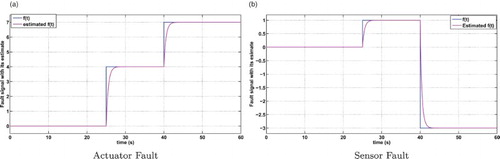
Table 1. Controller tuning parameters.

Sample time, Te	0.5 s
Prediction horizon,	8 Te
Control horizon,	6 Te
Input constraints
Output constraints	,
Input weights, R	0.1
Output weights, Q	1
Actuator fault matrix,
Sensor fault matrix,

Figure 3 shows the high precision of the actuator and sensor faults estimation. From Figure 4, it is shown that the nominal control law obtained using the FTC strategy is equal to before fault occurrence. Figure 5 illustrates the state estimation and Figure 6 illustrates the state tracking errors. Figure 7 shows the evolution of the activation functions. Through these figures, simulation results demonstrate the effectiveness and the applicability of the proposed FTC strategy even in the occurrence of actuator and sensor faults.

Figure 3. Faults and their estimates. (a) Actuator fault and (b) sensor fault.

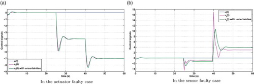
Figure 4. Nominal control and FTC of the uncertain faulty system vs. time. (a) In the actuator faulty case and (b) in the sensor faulty case.

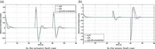
Figure 5. State estimation error signals vs. time. (a) In the actuator fault case and (b) in the sensor fault case.

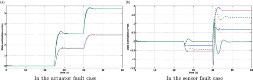
Figure 6. State tracking errors signals vs. time. (a) In the actuator fault case and (b)in the sensor fault case.

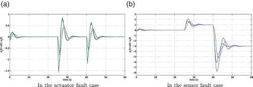
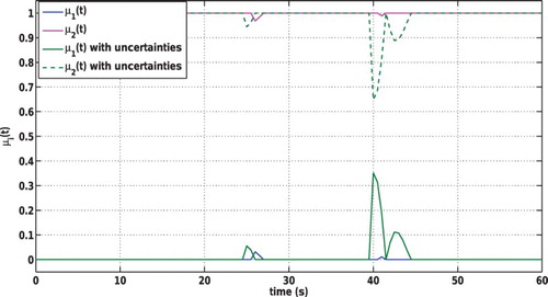
Figure 7. Membership functions evolution vs. time.

5. Conclusion

This paper has presented a fault-tolerant tracking controller for nonlinear uncertain systems. A T-S fuzzy observer is designed for the proposed strategy in order to estimate unmeasurable states and faults. Thus, the FMPC maintained good tracking performances between the faulty uncertain system and the healthy reference model. Infeasibility problems, instability and constraints dissatisfaction are not caused by the occurrence of faults. New sufficient conditions are developed for the existence of the robust FTC in terms of LMI constraints. From simulation results, we conclude that the proposed FTC strategy ensured nonlinear system stability and uncertainties on the model parameters.

Disclosure statement

No potential conflict of interest was reported by the authors.

Additional information

Funding

The authors gratefully thank ‘Ecole Doctorale Sciences et Techniques de l'Ingénieur de Tunis’, MESRST and ‘Région Haute Normandie’, FEDER for financially supporting this work within the framework of the VIRTUOSE project.

Appendix. Proof

Lemma .1.

Let us consider two matrices X and Y of appropriate dimensions. The following inequality is verified for each matrix Q (Ichalal et al., 2012):

Lemma .2

(Schur complement)

The following two inequalities are equivalent:

1. where and

2. .

The following Lyapunov's function is used for the Proof of the Theorem 3.1: (A1) where the matrix P is defined as follows: The derivative of is written as (A2) (A3) with . where denotes the Hermitian of the matrix X: . The derivative of the Lyapunov function is negative if the following inequality is satisfied , using the lemma of congruence as follows: (A4) The following inequality is obtained: (A5) where with . The inequality (A5(A3) ) can be written as (A6,A7) Using Lemma A.1, the inequality (A6(A4) ) becomes (A8,A9) where Θ is a symmetric definite positive matrix. Using Lemma A.2, we obtain the LMIs of Theorem 3.1, with and . The matrices , , and do not appear in the LMI after the variable change, its wise to choose them as identify matrices.

References

- Afonso, R. J. M., & Galvao, R. K. H. (2010). Predictive control of a helicopter model with tolerance to actuator faults. Conference on control and fault-tolerant systems, Nice, pp. 744–751.
- Aouaouda, S., Chadli, M., & Ichalal, D. (2013). Observer-based fault tolerant tracking control for vehicle lateral dynamics. IEEE international conference on control decision and information technologies, Hammamet, Vol. 5, pp. 051–056.
- Aouaouda, S., Chadli, M., M. T. Khadir, & T. Bouarar (2012). Robust fault tolerant tracking controller design for unknown inputs T-S models with unmeasurable premise variables. Journal of Process Control, 22(5), 861–872.
- Ben Hamouda, L., Bennouna, O., Ayadi, M., & Langlois, N. (2013). Quasi-LPV model predictive reconfigurable control for constrained nonlinear systems. Conference on control and fault-tolerant systems, Nice, pp. 590–595.
- Ben Hamouda, L., Bennouna, O., Ayadi, M., & Langlois, N. (2014a). Fuzzy model predictive reconfigurable control for nonlinear systems subject to actuators faults. International conference on automation and computing, Bedfordshire, pp. 140–145.
- Ben Hamouda, L., Bennouna, O., Ayadi, M., & Langlois, N. (2014b). Quadratic stability and LMIs for tolerance to faults: Fuzzy model predictive control. International conference on system theory, control and computing, Sinaia, pp. 387–392.
- Ben Hamouda, L., Bennouna, O., Ayadi, M., & Langlois, N. (2014c). Fuzzy fault tolerant control based on unmeasurable premise variables: Quadratic stability and LMIs. XVI Congreso Latinoamericano de Control Automático, Cancùn, pp. 319–324.
- Bergsten, P., & Palm, R. (2002). Observers for Takagi–Sugeno fuzzy systems. IEEE Transactions on Systems, Man and Cybernetics, Part B, (32), 114–121.
- Chadli, M., Aouaouda, S., Karimi, H. R., & Shi, P. (2013). Robust fault tolerant tracking controller design for a VTOL aircraft. Journal of the Franklin Institute, 350(9), 2627–2645.
- Fekih, A., & Seelem, S. (2015). Effective fault-tolerant control paradigm for path tracking in autonomous vehicles. Systems Science and Control Engineering, 3, 177–188.
- Ichalal, D., Marx, B., Maquin, D., & Ragot, J. (2012). Nonlinear observer based sensor fault tolerant control for nonlinear systems. IFAC Symposium on fault detection, supervision and safety of technical processes, Mexico City, pp. 1053–1058.
- Jamal Alden, M., & Wang, X. (2015). Robust control of time delayed power systems. Systems Science and Control Engineering, 3, 253–261.
- Johansson, M. (1999). Piecewise of linear control systems (PhD thesis). Department of Automatic Control, Lund Institute of Technology, Sweden.
- Kale, M. M., & Chipperfield, A. J. (2005). Stabilized MPC formulations for robust reconfigurable flight control. Control Engineering Practice Journal, 13(6), 771–788.
- Kumar Dohare, R., Singh, K., & Kumar, R. (2015). Modeling and model predictive control of dividing wall column for separation of Benzene-Toluene-o-Xylene. Systems Science and Control Engineering, 3, 142–153.
- Lofberg, J. (2004). Yalmip: A toolbox for modeling and optimization in MATLAB. IEEE in proceedings of the CACSD conference, Taipei, pp. 284–289.
- Maciejowski, J. M. (2002). Predictive control with constraints. Englewood Cliffs, NJ: Prentice-Hall.
- Nagy, A. M. (2010). Analyse et synthèse de multimodèles pour le diagnostic. Application à une station d'épuration (thesis). INPL, Nancy.
- Orjuela, R., Marx, B., Maquin, D., & Ragot, J. (2008). State estimation for non-linear systems using a decoupled multiple model. International Journal of Modelling Identification and Control, 4(1), 59–67.
- Orjuela, R., Marx, B., Ragot, J., & Maquin, D. (2009). Observer design for nonlinear systems described by multiple models. IFAC Symposium on fault detection, supervision and safety of technical processes, Barcelona.
- Rodrigues, M., Adam-Medi, M., Theilliol, D., & Sauter, D. (2008). A fault detection and isolation scheme for industrial systems based on multiple operating models. Control Engineering Practice Journal, 16, 225–239.
- Tanaka, K., Hori, T., & Wang, H. O. (2001). A fussy Lyapunov approach to fuzzy control and design. American control conference, Arlington, pp. 4790–4795.
- Tanaka, K., Hori, T., & Wang, H. O. (2003). A multiple Lyapunov function approach to stabilization of fuzzy control systems. IEEE Transactions on Fuzzy Systems, 4(11), 582–589.
- Tanaka, K., Ikeda, T., & Wang, H. O. (1996). Robust stabilisation of uncertain nonlinear systems via fuzzy control: quadratic stability, Hinf control theory and LIMs. IEEE Transactions on Fuzzy Systems, 4(1), 1–13.
- Tanaka, K., Ikeda, T., & Wang, H. O. (1998). Fuzzy regulators and fuzzy observers: relaxed stability conditions and LMI-based designs. IEEE Transactions on Fuzzy Systems, 6(2), 250–265.
- Takagi, T., & Sugeno, M. (1985). Fuzzy identification of systems and its application to modeling and control. IEEE Transactions. Systems, Man and Cybernetics, 15, 116–132.