Parametric covariance assignment using a reduced-order closed-form covariance model

ABSTRACT

This paper presents a novel closed-form covariance model using covariance matrix decomposition for both continuous-time and discrete-time stochastic systems which are subjected to Gaussian noises. Different from the existing covariance models, it has been shown that the order of the presented model can be reduced to the order of original systems and the parameters of the model can be obtained by Kronecker product and Hadamard product which imply a uniform expression. Furthermore, the associated controller design can be simplified due to the use of the reduced-order structure of the model. Based on this model, the state and output covariance assignment algorithms have been developed with parametric state and output feedback, where the computational complexity is reduced and the extended free parameters of parametric feedback supply flexibility to the optimization. As an extension, the reduced-order closed-form covariance model for stochastic systems with parameter uncertainties is also presented in this paper. A simulated example is included to show the effectiveness of the proposed control algorithm, where encouraging results have been obtained.

KEYWORDS:

• Reduced-order closed-form covariance model
• parametric covariance assignment
• stochastic systems
• eigen-decomposition

1. Introduction

Covariance analysis permeates almost all of system theory (Hotz and Skelton, 1987). Based on the covariance analysis, the couplings among random signals can be described. Therefore, the associated covariance control problem became one of the most significant research problems for multi-variable stochastic systems with the development of the stochastic control theory. Since the identification theory, Kalman filtering theory and model reduction theory are widely used in practice, the covariance estimation and control are significant to all of these research areas and applications (Åström and Eykhoff, 1971; Gelb, 1974; Rissanen and Kailath, 1972), while the covariance is an ideal tool to analyse the performance of the stochastic systems for both mean-square analysis and probabilistic decoupling analysis (Zhang, Zhou, Wang, and Chai, 2015).

During the past two decades, the covariance control theory (Hotz and Skelton, 1987) has made great progresses. The main result of this theory is based on the Lyapunov equation, and several conditions and controllers (Collins and Skelton, 1987; Grigoriadis and Skelton, 1997; Yasuda, Skelton, and Grigoriadis, 1993; Yaz and Skelton, 1991) have been proposed to control the covariance of the stochastic systems using the determined control signals. However, all of the controllers mentioned have no closed-form. Since the closed-form model of state covariance (Khaloozadeh and Baromand, 2007) presented in 2007, Baromand and Khaloozadeh designed different controllers and models (Baromand and Khaloozadeh,2010; Baromand and Labibi, 2012) to solve state covariance assignment (SCA) problem. All these literatures focus on the states of the stochastic systems rather than outputs of the stochastic systems and also the closed-form covariance model increases the dimension of the system variables from n-dimensional vector to -dimensional vector.

There are two unsolved problems remained so far using the closed-form model for covariance assignment problem. Firstly, the order of the controller must be more than the order of original systems which leads to the high-order controller, in addition, the computational complexity increases with it. For applications, the order of the controller is limited unfortunately, for example, the controller of the Hubble Space Telescope cannot be high order due to the limited space and computational complexity (Zhu, Grigoriadis, and Skelton, 1995). Secondly, the states cannot be measured in practice, thus how a controller can be designed using outputs of the stochastic control systems directly is still a challenging issue.

To solve these problems, this paper presents a novel reduced-order closed-form output covariance model for both continuous-time and discrete-time linear stochastic systems. With the proposed model, the order of the controller can be reduced comparing with the conventional covariance models and the computational complexity can be reduced. Moreover, the parameters of the proposed model are obtained using the Kronecker product operator and the Hadamard product operator directly. Based on this novel model, the state and output covariance control problems are simple to be solved with any state and output feedback control methods. To justify the feasibility and efficiency of the proposed model, the state and output covariance assignment problems are considered using parametric approaches (Konigorski, 2012; Roppenecker, 1986), which can supply flexibility to optimize covariance controllers. The main contributions of the work are characterized as follows: (1) using the eigen-decomposition approach, Kronecker product and Hadamard product, a novel reduced-order closed-form covariance control model has been presented; (2) based on this model, two parametric control algorithms are proposed for state and output covariance assignment problems; and (3) the extension of the presented model is developed for the stochastic systems with parameter uncertainties.

This paper is organized as follows: in Section 2, the reduced-order closed-form covariance model is presented. Section 3 presents two parametric feedback algorithms by the state and the output of stochastic systems. The numerical examples as simulations are given to illustrate the design produced and the usage of the presented model in Section 4. Finally, the reduced-order close-form covariance model is extended to stochastic systems with parameter uncertainties and conclusions are drawn in Sections 5 and 6, respectively. Meanwhile, the following notations will be used throughout this paper. denotes the vector-valued n-dimensional real space. denotes the covariance matrix of variable x. and are the real eigenvalue diagonal matrix and associated orthogonal matrix of , respectively. denotes the coefficient of the covariance model. U and Q are the covariance matrices of control input u and random noise w, respectively.

2. Reduced-order closed-form covariance model

In this section, a novel closed-form covariance model is presented using eigen-decomposition for continuous-time linear stochastic systems and discrete-time linear stochastic systems.

2.1. Discrete-time reduced-order covariance model

Consider the discrete-time linear stochastic systems subjected to Gaussian noises, which are represented as follows: (1) where and denote the state vector and output vector of the systems. is the control input vector and is the Gaussian noise vector. A,B,D and C are real constant matrices with appropriate dimensions.

Assume that the Gaussian noise vector satisfies:

H1 : , (2) where is the Dirac delta function.

Similar to the assumption of the noise, Baromand and Khaloozadeh (2010) assume that the control signal is restricted as (3) where .

Once the mean value of the control signal vector is restricted to zero, we have (4)

Based on the definition of the covariance matrix, the state and output covariance matrices of the given system are given by (5)

The covariance matrices can be restated using the system model and the associated dynamic Lyapunov equation is given by (6)

In Baromand and Khaloozadeh (2010) and Baromand and Labibi (2012), the covariance matrices are transformed to vectors using vectorization, which increases the order of the transformed model. To overcome this shortcoming, the eigen-decomposition is used to reduce the order of the model.

The covariance matrices are rewritten as follows: (7) where , , and are real diagonal matrices. , , and are associated orthogonal matrices. All of the matrices are with the same dimensions as the associated vectors.

The new formula of the dynamic Lyapunov equation can be obtained as follows: (8) where and .

Notice that for matrices G, F and with compatible dimensions, we have (9) where is the vectorization operator and ⊗ denotes Kronecker product (Liu and Trenkler, 2008).

Based on Equation (9(9) ), the dynamic Lyapunov equation can be transformed as follows: (10) where , , and .

Since the matrices and are diagonal, the associated vectors of and are with and zero elements, respectively. Thus, the elimination matrices and can be defined by (11) where , p=n,m.

Pre-multiplying and by and , the standard state-space model with uniform parameter expression can be given by (12)

where , , and denote eigenvalue vectors. The coefficient matrices can be calculated using Hadamard product (Liu and Trenkler, 2008) as follows: (13)

Remark 2.1.

It has been shown that Equation (12(12) ) satisfies the dynamic Lyapunov equation when the time trends to be infinite and the order of the model equals to the original system model.

2.2. Continuous-time reduced-order covariance model

Similar to the case of discrete-time system, the model for continuous-time systems is presented briefly.

Consider the continuous-time linear stochastic system subjected to Gaussian noise (14) where and denote state vector and output vector of the systems. is the control input vector and is the p-dimensional Wiener process. A,B,D and C are real constant matrices with appropriate dimensions.

Notice that the Wiener process is used to represent the integral of a Gaussian white noise process and it yields (15) where w is a standard Gaussian white noise.

Therefore, the system can be rewritten as follows: (16)

Compared with the assumption for the discrete-time system, the following assumption is given. H2 : , (17) where is the Dirac delta function.

Also, all the discrete-time variables defined above can be redefined as continuous-time variables by replacing k to t, and the covariance matrix for continuous-time system satisfies the following dynamic Lyapunov function: (18)

Using the similar approach, the eigenvalue matrix equation is given by (19) where and .

Notice that for matrices F and G with compatible dimensions, we have (20) where I denotes identity matrix.

Then, Equation (18(18) ) can be restated by vectorization as follows: (21)

Finally, using the elimination matrix (11(11) ), Equation (19(19) ) can be further expressed as a standard state-space model: (22) where , and can be obtained using Equation (13(13) ). Reserve the diagonal elements of which forms a diagonal matrix , then .

Remark 2.2.

For continuous-time linear stochastic systems, the output covariance assignment problem can be solved simply based on the proposed model following the approach similar to discrete-time linear stochastic systems. The design procedure and the illustrative example are certainly omitted here.

Remark 2.3.

The novel model presented in this section can be considered as the coordinate transformation of the original dynamic Lyapunov equation associated with the covariance matrix.

3. Parametric covariance assignment algorithms

Based on the reduced-order closed-form covariance model, the parametric state and output feedback control algorithms are developed to assign the covariance values. To simplify the contents of the paper, the control algorithms are proposed using a discrete-time model; on the other hand, the similar algorithms using a continuous-time model are omitted. The control objective of covariance assignment problem can be formulated as follows: (23) where denotes any pre-selected reference covariance matrix and is the state or output covariance matrix.

H3 : In this section, assume that the reduced-order closed-form covariance model is controllable.

3.1. State covariance controller design

For the SCA, the reference covariance matrix can be rewritten using eigen-decomposition as (24)

Since the diagonal matrix can be arranged as vector , the covariance assignment problem transfers to state tracking problem using the presented reduced-order covariance model if we set .

To track the desired state covariance vector, the integrator should be considered in the control scheme. The error vector is treated as the extended state and substitutes the error into the closed-loop system.

Then, the closed-loop system in the state-space form can be obtained as follows: (25) where

For this control system with error vector, a full-state feedback can be designed using a parametric state-feedback approach, which is presented by Roppenecker (1986) (26) and the feedback gain can be obtained by (27) where the modified parameter vectors are denoted by as free parameters.

In the case of a common open-loop and closed-loop eigenvalue, other parameters in Equation (27(27) ) can be determined as follows: (28) where and denote the open-loop eigenvectors and eigenrows of the model (25(25) ). and are given by model (25(25) ). is the kth column of the matrix . is a unit vector where the kth element is 1. In the other case, there is no common eigenvalue, , so that the parameters of Equation (27(27) ) can be selected by (29)

To reverse the transformation, can be obtained by and the actual control signal for original model can be given by (30) where denotes the standard Gaussian white noise.

Remark 3.1.

The actual control law is nonlinear though the original system model is linear.

Controller designing procedure can be summarized as Algorithm I:

Step 1. Choose the reference covariance matrix and calculating the eigenvalues and eigenvectors of the desired covariance matrix.

Step 2. Transform the stochastic systems from the original model to reduced-order closed-form covariance model.

Step 3. Transform the closed-form model to reference tracking model by adding the error vector.

Step 4. Choose poles and free parameters for closed-loop covariance control model and design the state covariance controller via parametric feedback approaches.

Step 5. Calculate the control signal for original systems using control law of covariance model.

Step 6. Substitute the control signal into the original systems.

3.2. Output covariance controller design

The output feedback is widely used when the system state cannot be measured. Similar to the state covariance controller design, the error vector should be introduced to these control systems, and the new state-space model with output equation can be described by (31) where

For this extended system, assume that the following conditions hold.

H4 : (Kimura's condition, Konigorski, 2012) .

The output feedback control law can be designed by a parametric output feedback approach, which is presented by Konigorski (2012) (32) and the feedback gain G can be obtained by (33) where can be calculated by kernel space and can be calculated by exterior algebra (see Konigorski, 2012 for calculation).

Once the control input is obtained, the actual control law can also be calculated by Equation (30(30) ).

The procedure of the controller design can be summarized as Algorithm II:

Step 1. Choose the reference covariance matrix and calculating the eigenvalues and eigenvectors of the desired covariance matrix.

Step 2. Transform the stochastic systems from the original model to reduced-order closed-form covariance model.

Step 3. Transform the closed-form model to reference tracking model by adding the error vector.

Step 4. Choose poles and free parameters for closed-loop covariance control model and design the output covariance controller via parametric feedback approaches.

Step 5. Calculate the control signal for original systems using control law of covariance model.

Step 6. Substitute the control signal into the original systems.

4. A numerical example

To verify this new model and the control algorithms proposed in this paper, one numerical example is presented in this section.

The original model can be shown as follows:

The covariance matrix of disturbance white noises is

To assign the covariance matrix, we choose the reference covariance matrix as

4.1. Case for state covariance

From the reference covariance matrix, the reference signal for covariance matrix eigenvalue model can be obtained as follows:

Simply, the reduced-order covariance model can be described as follows:

Based on this model and parametric state-feedback approach, the state covariance can track the given reference matrix by transformation and choosing different free parameter matrices

The state covariance feedback gain can be obtained as follows:

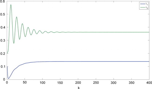
The results have been shown below. In Figures  1 and 2, the state covariance curves have been given using different feedback gains and . Both the control laws can assign the covariance to the reference covariance matrix; however, different free parameters of the controller lead to different performance. Figures 3 and 4 show the curves of the eigenvalues of the state covariance matrix, that is, the state vector of the reduced-order closed-form covariance model. From the curves, it has been shown that is better than for this example.

Figure 1. State covariance using .

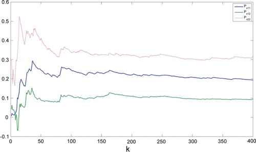
Figure 2. State covariance using .

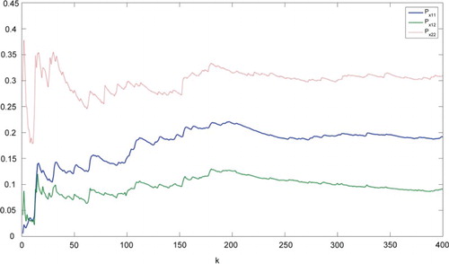
Figure 3. Eigenvalues of the state covariance matrix using .

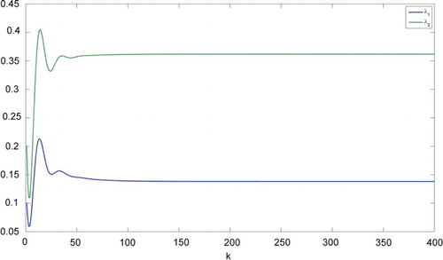
Figure 4. Eigenvalues of the state covariance matrix using .

4.2. Case for output covariance

As the above-mentioned approach, the eigenvectors can be chosen in the same way as and then we have

Based on this model and parametric output feedback approach, the output covariance can track the given reference matrix by transformation and choosing alternative free parameter matrix

Finally, the feedback gain can be calculated as follows:

To avoid repeating the results which is similar to the state covariance controller design, the curves for output covariance controller have been omitted.

Remark 4.1.

From the results of the simulation, different free parameters associated with the feedback gain bring different performance to the covariance model. It means that optimal free parameters can be obtained for a given performance criterion, such as minimum sensitivity and minimum control energy . The control algorithms presented in this paper can be extended simply which is helpful to apply in practice.

5. The reduced-order closed-form covariance model for stochastic systems with parameter uncertainties

In this section, the presented novel reduced-order closed-form model is extended for continuous-time and discrete-time stochastic systems with parameter uncertainties.

5.1. Discrete-time covariance model for stochastic systems with parameter uncertainties

Consider the discrete-time linear stochastic systems subjected to Gaussian noises, which are represented as follows: (34) where and denote state vector and output vector of the systems, respectively. is the control input vector and is the Gaussian noise vector. A,B,D and C are real constant matrices with appropriate dimensions. , , and are parameter uncertainties associated with A,B,D and C.

Using the similar operation, the reduced-order closed-form covariance model can be expressed as (35)

The parameter matrices can be obtained by Equation (13(13) ) and following equations: (36) where , , and .

5.2. Continuous-time covariance model for stochastic systems with parameter uncertainties

Consider the continuous-time stochastic systems with parameter uncertainties, which are subjected to Gaussian noise (37) where and denote state vector and output vector of the systems, respectively. is the control input vector and is the p-dimensional Wiener process. A,B,D and C are real constant matrices with appropriate dimensions. , , and are parameter uncertainties.

Thus, the reduced-order closed-form covariance model can be expressed as (38) where , and can be obtained using Equation (13(13) ). Reserve the diagonal elements of which forms a diagonal matrix , then . , and can be obtained by Equation (36(36) ). Similarly, .

Remark 5.1.

Due to the fact that the covariance model and original system model are the same in form, the robust control algorithms can be applied to solve the covariance control problem. Moreover, this model can be reduced as models (12(12) ) and (38(38) ) if the parameter uncertainties are zeros, which implies that the covariance model with parameter uncertainties can be considered as an extension to models (12(12) ) and (38(38) ).

6. Conclusions

For continuous-time and discrete-time stochastic systems subjected to Gaussian white noises, a novel model for state and output covariance assignment problems has been proposed using eigen-decomposition in this paper which are named the reduced-order closed-form covariance model. The coefficient matrices of this presented model can be obtained by uniform formulas which imply the uniform expression. Based on this model, two nonlinear control laws have been formulated following two presented control algorithms by parametric state-feedback approach and parametric output feedback approach, where the free parameters can be further used to optimize other control criterion.

Moreover, the presented model is also extended to stochastic systems with parameter uncertainties. With the numerical example, it has been shown that the covariance assignment problem can be solved effectively using the presented reduced-order closed-form covariance control model. Based upon this novel model, some further advanced topics can be investigated as future works, for example, the proposed control algorithm can be extended using the non-fragile state estimation (Hou, Dong, Wang, Ren, and Alsaadi, 2016; Yang, Dong, Wang, Ren, and Alsaadi, 2016; Yu, Dong, Wang, Ren, and Alsaadi, 2015), while the robustness of the control algorithm for covariance assignment problem is enhanced.

Acknowledgments

The authors would also like to thank the editor and the reviewers for their kind advice about this paper.

Disclosure statement

No potential conflict of interest was reported by the authors.

Additional information

Funding

The authors acknowledge the National Natural Science Foundation of China [grant number 61573022], [grant number 61290323] and [grant number 61333007].

References

- Åström, K. J., & Eykhoff, P. (1971). System identification – a survey. Automatica, 7(2), 123–162. doi: 10.1016/0005-1098(71)90059-8
- Baromand, S., & Khaloozadeh, H. (2010). On the closed-form model for state covariance assignment problem. IET Control Theory and Applications, 4(9), 1678–1686. doi: 10.1049/iet-cta.2009.0546
- Baromand, S., & Labibi, B. (2012). Covariance control for stochastic uncertain multivariable systems via sliding mode control strategy. IET Control Theory and Applications, 6(3), 349–356. doi: 10.1049/iet-cta.2010.0625
- Collins Jr., E. G., & Skelton, R. E. (1987). Theory of state covariance assignment for discrete systems. IEEE Transactions on Automatic Control, AC-32(1), 35–41. doi: 10.1109/TAC.1987.1104443
- Gelb, A. (1974). Applied optimal estimation. Cambridge, MA: MIT Press.
- Grigoriadis K. M., & Skelton, R. E. (1997). Minimum-energy covariance controllers. Automatica, 33(4), 569–578. doi: 10.1016/S0005-1098(96)00188-4
- Hotz, A., & Skelton, R. E. (1987). Covariance control theory. International Journal of Control, 45(1), 13–32. doi: 10.1080/00207178708933880
- Hou, N., Dong, H., Wang, Z., Ren, W., & Alsaadi, F. E. (2016). Non-fragile state estimation for discrete Markovian jumping neural networks. Neurocomputing, 179, 238–245. doi: 10.1016/j.neucom.2015.11.089
- Khaloozadeh, H., & Baromand, S. (2007). State covariance assignment problem. IET Control Theory and Applications, 4(3), 391–402. doi: 10.1049/iet-cta.2008.0359
- Konigorski, U. (2012). Pole placement by parametric output feedback. Systems and Control Letters, 61(2), 292–297. doi: 10.1016/j.sysconle.2011.11.015
- Liu, S., & Trenkler, G. (2008). Hadamard, Khatri-Rao, Kronecker and other matrix products. International Journal of Information and Systems Science, 4(1), 160–177.
- Rissanen, J., & Kailath, T. (1972). Partial realization of random systems. Automatica, 8(4), 389–396. doi: 10.1016/0005-1098(72)90098-2
- Roppenecker, G. (1986). On parametric state feedback design. International Journal of Control, 43(3), 793–804. doi: 10.1080/00207178608933503
- Yang, F., Dong, H., Wang, Z., Ren, W., & Alsaadi, F. E. (2016). A new approach to non-fragile state estimation for continuous neural networks with time-delays. Neurocomputing, 197, 205–211. doi: 10.1016/j.neucom.2016.02.062
- Yasuda, K., Skelton, R. E., & Grigoriadis, K. M. (1993). Covariance controllers: A new parametrization of the class of all stabilizing controllers. Automatica, 29(3), 785–788. doi: 10.1016/0005-1098(93)90075-5
- Yaz, E., & Skelton, R. E. (1991, December 11–13). Continuous and discrete state estimation with error covariance assignment. Proceedings of the 30th IEEE conference on decision and control (Vol. 3, pp. 3091–3092), Brighton.
- Yu, Y., Dong, H., Wang, Z., Ren, W., & Alsaadi, F. E. (2015). Design of non-fragile state estimators for discrete time-delayed neural networks with parameter uncertainties. Neurocomputing, 182, 18–24. doi: 10.1016/j.neucom.2015.11.079
- Zhang, Q., Zhou, J., Wang, H., & Chai, T. (2015, December 15–18). Minimized coupling in probability sense for a class of multivariate dynamic stochastic control systems. Proceedings of the 54th IEEE conference on decision and control (pp. 1846–1851), Osaka.
- Zhu, G., Grigoriadis, K. M., & Skelton, R. E. (1995). Covariance control design for Hubble space telescope. Journal of Guidance, Control, and Dynamics, 18(2), 230–236. doi: 10.2514/3.21374