System science and control techniques for harnessing nuclear energy

ABSTRACT

Scientists and researchers are optimistic about safe usage of nuclear power even after several accidents. The control system is a crucial subsystem of the reactor, and accounts for its safe operation. In this review article, several types of control problems in nuclear reactors are presented and discussed, particularly the direct and indirect effects of temperature changes on the reactivity. The first part of the article describes the architecture for instrumentation and control, and outlines various reactivity feedback. Nuclear fuel handling control and turbine speed control are illustrated. The second part considers simulation techniques used in practice, including simulations of the effects of internal feedback and external reactivity perturbations, simulation techniques used to model the different types of problems, and the control schemes used to control reactor parameters. The paradigm of each control algorithm is explained. Techniques to simulate or to model a reactor coupled with different types of loads are explained.

KEYWORDS:

• Nuclear power
• reactivity implications
• control

1. Introduction

Fission of an U²³⁵atom by a thermal neutron releases two fragments, 2 or 3 neutrons, and ∼200 MeV of energy (Figure 1). In a reactor that is operating at a steady state, the rates of production and loss of neutrons are balanced exactly and the reactor power remains constant in time. Any deviation in this balance by mechanisms like control rod motion, flow changes, or fuel burn-up will cause the power output to vary over time. The study of this transient behaviour is referred to as reactor kinetics. Studies of reactor kinetics and reactor control can be used in designing a safe nuclear plant or maintaining its safety margins. The purpose of this article is to list all factors that can cause reactor operation to deviate from steady state, and control schemes that can be used to return reactor operation to a steady state.

Figure 1. Fission of a ²³⁵U atom.

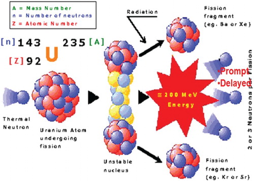
Neutrons that appear within 10⁻¹⁷ s of the fission event are called prompt neutrons; these can be assumed to appear instantaneously. Neutrons that appear long after the fission event are called delayed neutrons; they constitute a very small fraction, β, of the total neutron population (0.65% for ²³⁵U). Delayed neutrons originate in the decay by neutron emission of nuclei that are produced following beta-decay of fission fragments. Production of prompt neutrons in an overcritical reactor system can lead to accidents. Production of delayed neutrons (that appear within few milliseconds to a few minutes) makes the chain reaction controllable.

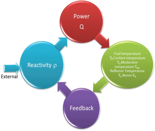
The reactor core is composed of several entities, including fuel segments or blocks, coolant, moderator, and reflector which are packed together inside a pressure vessel; all of these are enclosed by a containment building. Reactor power is mainly controlled by changing the position of the control rods, which in turn varies the sensitive parameter known as reactivity ρ = (k−1)/k, where k is stated as the ratio of the neutrons generated by fission in one generation to the number of neutrons lost through absorption and leakage in the preceding generation. The temperatures of the fuel, coolant, moderator, and reflector are interdependent and they change cyclically as shown in Figure 2. The amount of external ρ to be added by using the control rods depends on the instantaneous power of the reactor.

Figure 2. Physical phenomenon.

Technologies in industrial environment to manage process measurement, condition monitoring, predictive maintenance, plant safety, internal communication, and personnel monitoring have been evolving rapidly. If wireless technology is used in the nuclear plants then sensors and signals can be supplied without cost or requiring time to evaluate, install, and manage the wiring and conduits, but the nuclear industry is slower to adopt new technologies than are other industries, because the nuclear industry is dedicated to safety and must ensure defense in depth against any problem that use of a new technology could cause.

The control systems, including control rods design, are the most important part of the reactor system. Human interaction with human-machine interface can be error-prone; therefore an automatic control system can be used to eliminate such errors. In this article, the necessity of precise control in reactor operation is established by Section 2, by analysing the Chernobyl reactor accident. Section 3 outlines the hardware design of control systems for nuclear reactors. Section 4 explains the basics of reactivity phenomena, and Section 5 explains various simulation techniques used to solve engineering problems for accessing nuclear energy.

2. Necessity of precise control

The necessity for precise control is exemplified by the Chernobyl accident that happened on 26 April 1986. The Reaktor Bolshoy Moshchnosti Kanalnyy type of reactor had been built in Chernobyl, Ukraine, by the Soviet Union. The reactor had a power rating of 3200 MWt. Designers claimed that the residual momentum and steam pressure were sufficient to run the coolant pumps for 45 s, eliminating the time duration between an external power failure and the full availability of the emergency generators. This capability was required to be confirmed experimentally for the reactor at Chernobyl. The reactor was under manually operated control. A part of the experimental procedure entailed conducting a steam turbine experimental test at 800 MWt of power; so the operator reduced the reactor power from 3200 to 800 MWt, but the control system did not account for the Xenon poison, which has an absorption cross-section of ∼2.65 × 10⁶ barns at 0.025 eV. Thus, the reactor power went on reducing automatically and reached 30 MWt (Figure 3).

Figure 3. Reactor power against time.

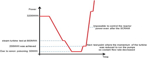
To perform the experimental test the operator decided to increase the reactor power. The control system could not raise the reactor power back to the 800 MWt level due to increased Xenon poisoning even after pulling out the control rod, but somehow the operator managed to raise the power to 200 MWt. Four Main Circulating Pumps (MCPs) were in active condition out of six active MCPs used during regular operation. Also, the reactor was designed with a positive feedback of void (steam void/bubble) coefficient of reactivity. The prompt power rise was initiated by a low coolant flow rate. This caused water to boil. Officials decided to perform the steam turbine test at the 200 MWt power level, but the reactor was unstable at that power level. The control system could not control the reactor power even after the SCRAM (an emergency shutdown) operation. The leading edge of the control rod contained a graphite tip that had no neutron absorber and that moved out of the neutron-absorbing fluid (water); as a result the reactivity was increased and the reactor power increased drastically (Figure 3). Two prompt neutron spikes of increasing amplitudes were generated; these raised the reactor power from 200 to 3800 MW and then to 120 times the rated power of the reactor (Lee & Mc Cormick, 2011), and the reactor was totally out of control. Thus, the key challenges in core power control to assure safety and reliability are to:

1. Control displacement of the control rods exactly.

2. Control the reactor power while preserving neutron flux profile. But reactor power is a function of the reactivity, which is a function of the temperatures of the fuel, coolant, moderator, and reflector; therefore to maintain power, these parameters must all be controlled.

3. Control the coolant mass flow rate.

With the advances in nuclear science and engineering, methods to overcome these challenges are available. Practically, an instrumentation and control (I&C) system is used to control the nuclear plant, but simulation studies with a nuclear plant are used to predict how a reactor will behave during transient or accident scenarios. The nuclear power plant (NPP) control also involves control for fuel handling, turbine speed control, and other processes which are completed manually. Simulation studies are very important both for design calculation during the normal operation and for taking precautions against accident scenarios.

3. Instrumentation and control

3.1. Control room

A modern digital I&C system mainly manage two tasks.

1. Reduction of the operator’s workload by using computerized control.

2. Reduction of the maintenance work load by using self-diagnosis functions.

The architecture for I&C (Figure 4) can be subdivided into four subsystems.

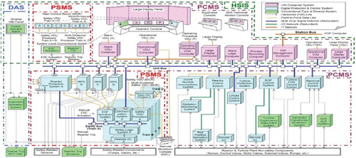
1. The protection and safety monitoring system (PSMS) used for safety functions.

2. The plant control and monitoring system (PCMS) used for non-safety functions.

3. The diverse actuation system (DAS) in analogue form used for protection against software common cause failure in PSMS and PCMS.

4. The human–system interface system (HSIS) used by the operator to interact with PSMS, PCMS, and DAS.

Figure 4. Overall architecture of the I and C system (Kenji & Hiroshi, 2014).

This modern architecture for the I&C system has the following advantages.

Reliability: Redundancy in the architecture leads to reliable operation of the I&C system. Human efficiency is enhanced by using a multi-division operator workstation. This system can be used for sustained operation; it has been tested without unplanned outage from equipment failure.

Maintainability: The surveillance workload is reduced substantially by including extensive self-diagnosis features. The number of spare parts is reduced by using a standardized digital platform.

Simplicity: Use of visual display units means that safety functions can be easily overviewed at a glance. Extensive usage of data communication provides correlations among various subsystems and simplifies decision-making processes.

3.2. Control rod position monitoring system

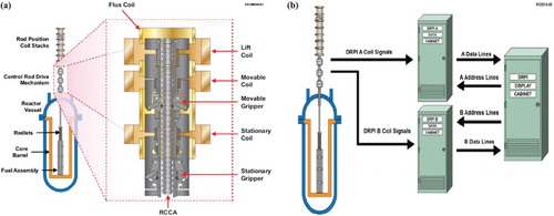
The pressurized water reactor (PWR) control rod drive mechanism manufactured by L&T and other organizations has a set of coils; the control rod is moved by using regulated DC voltage to apply a magnetic field in the coils. The energy required to hold, withdraw, or insert each of the control rods is given by regulated voltage signals that are produced outside containment at the rod control cabinet. The digital control rod position indicator (DRPI) also has a coil stack which is set up on top of the control rod drive mechanism system (Figure 5(a)). Forty-two individual coils are present inside each coil stack, and are excited by an AC voltage. These 42 coils are divided into two groups: DPRI A and DPRI B. Both the groups are inter-spaced with a distance of six steps of control rod drive mechanism (CRDM). The DRPI data cabinets are placed inside a containment building and are used to monitor the coil currents and convert them to digital form (Figure 5(b)). The DPRI display cabinet in the control room continuously sends a seven-bit control rod address to the data cabinets while the corresponding data cabinet sends the six-bit control rod position.

Figure 5. Control rod drive position monitoring system. (a) Digital control rod position indicator. Rod positioning coil stack is placed on top of the CRDM system (Hashemian, Morton, & Shumaker, 2009) and (b) digital control rod position indicator. Signal flow between DRPI coils, data cabinet and display cabinet (Hashemian et al., 2009).

For a crucial CRDM system, reliability testing must be performed by observing the latch time of the stationary gripper of CRDM. The reliability should be determined by observing the consistency of the results from rod to rod, step to step, and plant to plant. Data containing faults are compared with reliable data. Thus, any actual or induced fault is identified.

3.3. Control rod worth

The reactivity changes very little per unit distance when the control rods are just introduced into a reactor or completely inserted into it (Figure 6). The main reason for this phenomenon is that the flux is very small and therefore the rods absorb few neutrons during the transient; hence the effect of control rods when neither inserted completely nor fully withdrawn must be considered. Reitsma et al. measured the reactivity of the control rods for a pebble bed reactor at ASTRA Critical Facility at the Russian Research Centre (Reitsma & Naidoo, 2003).From Figure 6, reactivity changes can be observed.

Figure 6. Differential reactivity worth of the CR5 control rod (Nojiri, Shimakawa, Fujimoto, & Goto, 2004).

3.4. Digital computer-based automatic control

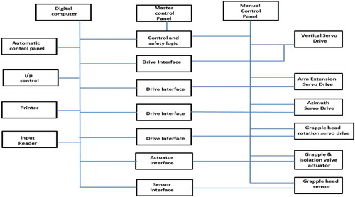
The reactor is refuelled by removal of depleted fuel blocks and the addition of fresh fuel periodically. The controlling process to achieve this purpose is explained with an example of digital computer-based automatic control for a high-temperature gas-cooled reactor (HTGR) at Fort St. Vrain which is shut down presently. Automatic control of the fuel-handling process is approximately five times faster than manual operation using the same machine. Moreover, operator errors are eliminated, and an accurate log of all fuel movements is recorded. The refuelling system for the Fort St. Vrain Nuclear Generating Station used a small digital computer to automatically control the distributions and positions of the approximately 3000 fuel and reflector blocks that constitute the reactor core (Smith & Mathie, 1973). The computer had complete control of the handling mechanism, including four degrees of freedom in motion. For inventory purposes, the computer also logged information concerning all fuel movements. The HTGR core was designed to produce 330 MWe power, and contains about 3000 removable reflectors and fuel blocks located inside a pre-stressed concrete pressure vessel. Each year, about one-sixth of the fuel blocks in the reactor were replaced.

The important consideration in this control system was to maintain a fail-safe condition throughout operation and to prevent operator error. Hence, extensive hardware interlocks and failure detection devices were used (Figure 7). This safety system was functional in automatic, manual, and semi-automatic modes of operation. An annunciator was supplied with 50 status and alarm messages to warn the operator about any problem that could occur and provided guidance to take corrective actions. The software could control all machine functions, but needed sequence and coordinate data input before initiating a cycle of fuel block management. Changes to the refuelling process or sequence could be made without reassembling the computer software system. The position feedback in digital format was read into the computer; this issued a digital positioning command, and then controlled the velocity of the drives while they were moving. A position error signal was evaluated by digitally subtracting the commanded position from the position provided by shaft encoders in the drive system. Motors were driven by the analogue signal obtained from conversion of the corresponding digital error signal. The computer used the relay contact outputs to control the grapple and the cask isolation valve. Machine status was provided by various contact inputs to the computer. The control system could be operated in Automatic, Semi-automatic, or Manual modes.

Figure 7. Hardware block diagram for handling hexagonal blocks.

3.5. Distributed control system for turbine control

In a secondary side or power conversion system of the nuclear plant, control of the turbines is essential to ensure safe operation of a nuclear reactor. The intent of the system is to preclude damage to turbines, which must be run below a certain angular velocity. During generation of AC electricity, the speed of the turbine must be controlled precisely. An over-speed trip can occur when the acceleration of the turbine rotor is out of control. In the over-speed scenario, the nozzle valves that control the flow of steam to the turbine must be closed. When this corrective action fails, the turbine may continue to accelerate until it breaks apart, often with unfortunate consequences. Turbines are among the most expensive components used in the NPP, and are manufactured from special-quality materials. The old analogue technology in the Turbine Control of Bruce Nuclear Plant Unit 1 and Unit 2 has been replaced by a distributed control system due to equipment ageing, unavailability of parts, high maintenance, and numerous turbine trips (Gray & Basu, 2009). A distributed control system uses remote main control processors and local valve control processors. To minimize signal losses and noise, a local panel is located on the turbine deck and all signals are sent to the remote control equipment room panel via redundant fibre optics (Figure 8).

Figure 8. Distributed control system for turbine control. (a) Turbine overall layout (Gray & Basu, 2009). Upgrade of the turbine control system for Bruce nuclear plant units 1 and 2 and (b) Distributed control system overview in Gray and Basu (2009).

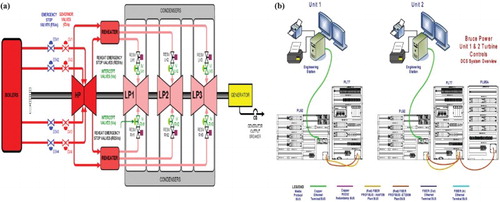
Benefits of this distributed control system include increased safety margin, availability, and reliability because of redundancy of components and on-site availability of spare parts. With the mean down time (MDT) of 4 h, that is, 4.566×10⁻⁴ y and mean time between failures (MTBF) of 37.7 y, the availability becomes

4. Reactivity implications

Reactivity determines the rate at which the reactor power changes. As fissile materials such as U²³⁵and Pu are consumed, fission products build up; these include Xenon, which can damp (poison) the reaction. Also, the temperatures of the fuel, heat transport fluid (coolant), and moderator change during reactor operation. The changes in reactivity that result from temperature changes must be considered. The formation of voids in the coolant or moderator due to boiling or accidental loss of fluid is closely related to temperature changes. Therefore, void formation and its effect on reactivity also must be considered.

The Temperature Coefficient of Reactivity is defined as the change in reactivity per unit increase in temperature (mk/°C). Temperature changes occur not only in fuel and in the heat transport system but also in the moderator and therefore temperature coefficients for each separate material must be considered (Bel & Glasstone, 1970; Duderstadt & Hamilton, 1976; Glasstone & Sesonski, 1963; Lamarsh, 1966; Lewis, 1977). To ensure that the reactor is self-regulating, the overall temperature coefficient should be negative.

Reactivity can change with temperature. Factors that cause these changes can be divided into three main categories as follows.

I. Mechanical changes

Temperature changes cause decrease in density of the moderator and of the heat transport fluid. These changes reduce the rate at which neutrons are slowed down and captured; therefore the diffusion length increases and the chances of the neutrons escaping increase, so reactivity decreases.

II. Direct nuclear effects

Temperature changes cause Doppler Broadening, which describes the effect of thermal energy on the probability that a neutron will strike a target nucleus. The probability that resonance capture occurs at neutron energies is calculated with the assumption that the target nucleus is at rest. If the uranium is hot and the nuclei are vibrating rapidly, a neutron that would be outside the resonance peak may encounter a nucleus which is moving at the necessary speed to put their relative velocity in the resonance peak. Thus the neutron, which might have escaped cold fuel, is captured when uranium is hot and there is decrease in resonance escape probability (); as a consequence the reactivity decreases.

III. Indirect nuclear effects via neutron temperature

Temperature in the reactor also affects the neutron temperature. The thermal neutrons in a reactor core have a distribution of energies that approximates the Maxwellian distribution of energies of molecules. Any increase in temperature of the fuel, heat transport fluid, or moderator will in turn raise the energies of thermal neutrons that enter the fuel and thereby increase their temperatures; this change can cause decrease or increase in reactivity depending on the type of reactor.

4.1. Temperature reactivity coefficients

4.1.1. Fuel temperature coefficient of reactivity

The reactivity changes due to increased fuel temperatures are mainly due to (i) increase in the effective temperature of the thermal neutrons causing a reduction in the number of neutrons produced per neutron absorbed for fully irradiated fuel and (ii) increase in resonance capture, with a resulting reduction in resonance escape probability (p) due to Doppler Broadening.

In a reactor that uses the same type of fuel throughout its core, the fuel temperature coefficient is expressed as the milli-k change in reactivity per °C (or °F). Because of the above effects, the expected values for a Douglas Point nuclear plant for equilibrium fuel are in the micro-k range (Table 1).

Table 1. Bifurcation of reactivity changes.

Parameter	Reactivity (mk/°C)
Neutron temperature	+0.0036
Doppler effect	−0.014
Total fuel temperature coefficient	−0.0104

When the fuel temperature coefficient is negative, excess reactivity must be provided in the reactor to balance the decrease in reactivity that occurs as the fuel heats up when the reactor power is increased.

4.1.2. Coolant temperature coefficient of reactivity

An increase in the temperature of the heat transport system will result in a change of reactivity because:

1. The temperature increase again causes an increase in neutron energy with the same results as with the fuel temperature coefficient above and

2. A reduction in density causes an increase in thermal utilization (f), fast fission factor (), and decrease in resonance escape probability (p).

The overall heat transport temperature coefficient is usually negative with fresh fuel but becomes progressively less negative as the fuel is consumed. The problem in returning to high power following a reactor trip is generated by a negative value for this coefficient; so should such a trip occur, the heat transport temperature should be kept as high as possible until the reactor is back at high power. To keep temperature high, the steam generator must be isolated from the turbine, so that heat from the heat transport system is not being used to produce steam for the turbine. When the algebraic sum of the fuel and heat transport temperature coefficients is positive, the reactivity increases as reactor power increases and the problem of returning to high power following a reactor trip does not occur, but such a system is less stable because a transient increase in power leads to a rise in temperature which results in an increase in reactivity which tends to raise the power further.

4.1.3. Moderator temperature coefficient of reactivity

Changes in reactivity with increase in moderator temperature are mainly caused by

1. Increase in the effective neutron temperature with the same results as with the fuel temperature coefficient above.

2. Reduction in moderator density with resulting increase in diffusion length () and hence in neutron leakage. Reduction in moderator density also causes a decrease in p and an increase in thermal utilization f. With new fuel, the moderator temperature coefficient is negative. A negative moderator temperature coefficient would allow some additional reactivity to be obtained, to help counteract a Xenon transient following a reactor trip, by cooling the moderator.

4.1.4. Effects due to void formation

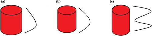
Voids are formed if either the moderator or heat transport system boils. This boiling could be caused by an increase in heat generation, a decrease in cooling flow, or a reduction in pressure due to a failure in the system. Usually, if a reactor is over-moderated, that is, with moderator/fuel ratio in excess of that needed to just thermalize the neutrons, then a void can form in the moderator, and this void will cause an increase in reactivity. If the reactor is not over-moderated, an increase in reactivity can still result. The size of the void and its location are significant in determining whether its formation will cause an increase or decrease in reactivity.

The void coefficient of reactivity is defined as the change in reactivity per 1% change in water (coolant) volume. Excessive positive or negative void coefficients should be avoided if possible. An excessively large positive coefficient will generate large power surges during the void formation, and the surges will cause severe damage to the reactor if the protective system does not respond quickly enough. In contrast, excessively negative coefficients cause a rapid decrease in power when the void is formed; the decrease is corrected by the regulating system, but when the void fills, a power surge results.

4.2. Reactivity effects due to fuel irradiation

The long-term reactivity effects arise due to changes occurring in the fuel as a result of fuel irradiation. These changes are: (i) accumulation of fission products in the fuel and (ii) burn-up of ²³⁵U and build-up of Pu. These can also cause a transient change in reactivity on reactor shutdown which can affect the availability of the reactor in a base load station.

Most of the fission products are classified as reactor poisons because they all absorb neutrons to some extent. However, the two most important poisons are ¹³⁵Xe and ¹⁴⁹Sm. They have very large thermal neutron capture cross-sections and therefore cause substantial changes in reactivity as they build up in the fuel. The one important difference between them is that ¹³⁵Xe is radioactive, whereas ¹⁴⁹Sm is stable. The two isotopes will be discussed separately.

4.2.1. Xenon oscillations

During the reactor operation, Xenon is produced in two ways (Figure 9, Table 2):

1. Directly as a fission product and

2. Indirectly from the decay of ¹³⁵I which, in turn, is produced as a fission product or from the decay of fission product ¹³⁵Te.

Figure 9. Xenon chain.

Table 2. Parameters for the Xenon chain.

Parameter
Fission yield	0.0639	0.00237
Decay constant (s^−1)

The time dependence of the concentrations of ¹³⁵I and ¹³⁵Xe based on the simplified scheme can be written as (1) (2) where is the macroscopic fission cross-section in fuel, is the microscopic absorption cross-section in Xenon, and is the space-averaged flux. Following terms are used to explain the Xenon oscillations (Lee, Jones, & McCoy, 1971).

1. Axial shape index (ASI): This is the ratio of the difference between the core power P_B at the bottom and the core power P_T at the top to the sum of these powers: (3)

2. Equilibrium shape index (ESI): This is the value of the ASI determined at rated power with equilibrium Xenon concentration when all the control rods are withdrawn. Axial offset (AO) and ASI are interchangeable terms.

The equilibrium flux profile of the core is dependent on the age of the reactor core (Figure 10). In a new core the flux peak is nearer the bottom of the core than the top due to the initial condition of the control rods or the negative moderator temperature coefficient of the reactivity.

Figure 10. The sketches for flux changes of the PWR core with respect to age of the core.

As the fuel is consumed, the flux peak shifts towards the centre of the core. Thus, during the middle age of the core, the flux profile of the core follows the chopped cosine distribution. Over time, the fuel in the centre of the core gets burned more than the fuel at the top and bottom; so near the end of the core lifespan, a bimodal flux profile is generated with one peak in the top of the core and another peak near the bottom of the core. The axial oscillations of Xenon can be explained as follows.

Let the initial flux profile of the core be as illustrated in Figure 11(a). When the control rods are inserted, the flux profile of the core is changed to that as in Figure 11(b). The amplitude of the flux is lower in the top position than in the bottom; so less Xenon is burned out in the top than in the bottom. Moreover, the iodine (¹³⁵I) decays to ¹³⁵Xe; so the concentration of the ¹³⁵Xe increases in the upper zone of the core (Figure 11(c)). As the Xenon concentration increases, the reactivity in the top of the core decreases and the fission power is consequently reduced. In contrast, the increased power in the lower zone burns more ¹³⁵Xe than in the upper zone; this process decreases the ¹³⁵Xe concentration in the lower zone and consequently further increases the core power in the lower zone (Figure 11(c)).

Figure 11. Xenon build-up in an asymmetrical manner over the period in the PWR.

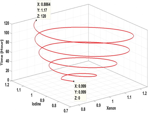
Because the fission yield of Iodine ¹³⁵I is 6.39% (more than that of ¹³⁵Xe), more ¹³⁵I than ¹³⁵Xe is produced in the lower zone of the reactor core. This ¹³⁵I eventually decays to ¹³⁵Xe. This reduces the fission power in the lower zone (Figure 11(d)). The Xenon oscillation has a period of ∼30 h. The Xenon oscillations can be convergent (Figure 11(e)) or divergent (Figure 12). These oscillations can be dampened by appropriate insertion of the part length control rod. ASI should be usually maintained within 0.05 units of the ESI value. The free running oscillations of Xenon on the phase plane of Xenon and Iodine are depicted in Figure 13. The time-optimal control to kill the spatial Xenon oscillation was obtained by Schulz and Lee (1980).

Figure 12. Diverging Xenon or flux oscillations.

Figure 13. Oscillations of Xenon and Iodine after external perturbation in the upper half of the reactor core.

Schulz et al. have presented Xenon oscillations in the equilibrium state as or , where control input is constrained as . The state vector is defined as , where and denote Xenon and Iodine amplitude, respectively, and A, B are coefficient matrices (Schulz & Lee, 1980).

The concentrations of Xenon before and after the shutdown are shown together in Figure 14 for the average flux value of 10¹⁴/cm² S. As illustrated the steady-state Xenon concentration reaches an equilibrium level after the start-up of the reactor at about 10⁵s. This concentration induces reactivity of about 4$. The Xenon concentration starts increasing after the shut down, and reaches a maximum at 10.29 h after shutdown (Figure 14).

Figure 14. Xenon concentration before and after shutdown (S) for an average flux of 10¹⁴/cm² s.

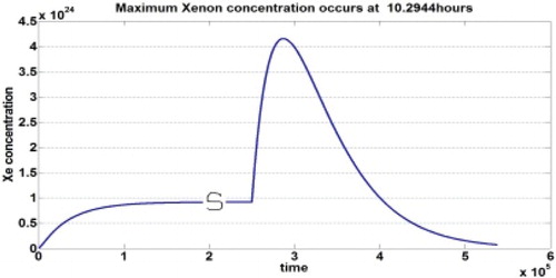
When the reactor power is decreased or shut down by inserting neutron-absorbing control rods, the neutron flux is reduced and the ¹³⁵Xe concentration starts increasing. The ¹³⁵Xe concentration peaks at about 10.29 h after the shutdown. Because ¹³⁵Xe has a 9.2-h half-life, the ¹³⁵Xe concentration takes >72 h to decay to low levels.

The temporarily high level of ¹³⁵Xe with its high neutron absorption cross-section makes it unmanageable to restart the reactor for several hours. The neutron absorbing ¹³⁵Xe acts like a control rod, reducing the reactivity. The inability of a reactor to be started due to the effects of ¹³⁵Xe is called as Xenon precluded start-up and the duration of time for which the reactor is unable to override the effects of ¹³⁵Xe is called the reactor or Xenon dead time (Figure 15).

Figure 15. Xenon reactivity.

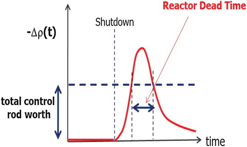
For a reactor that has a negative moderator temperature coefficient of reactivity, some of the required additional reactivity can be supplied by cooling the moderator. Nonetheless, the best method of providing this reactivity is to insert extra fuel, in the form of a booster rod, into the reactor during the reactor dead time. Booster rods have been widely used in Indian nuclear reactors, but use of a booster rod prevents some amount of fuel in the core because the booster rod is only used after the shutdown.

4.2.2. Build-up of samarium poison

Among the stable poisons, the most notable is ¹⁴⁹Sm, which is formed by the decay of ¹⁴⁹Pm, which is formed by decay of ¹⁴⁹Nd. ¹⁴⁹Sm poison reaches its equilibrium in much the same way as ¹³⁵Xe. Because ¹⁴⁹Sm is stable it is not removed by decay and its rate of removal by neutron capture is slower than that of Xenon. Nonetheless, ¹⁴⁹Sm accumulates more slowly than ¹³⁵Xe, and therefore reaches equilibrium more slowly than does ¹³⁵Xe. The ¹⁴⁹Sm equilibrium load is only slightly greater than 0.2 times that of ¹³⁵Xe (Henry, 1997).When the reactor trips, or is shut down, the concentration of ¹⁴⁹Sm increases much in the same way as the ¹³⁵Xe. However, because ¹⁴⁹Sm does not decay, it continues to increase until all the ¹⁴⁹Pm has decayed. The maximum ¹⁴⁹Sm load will be two or three times the equilibrium operating load.

5. Simulation techniques

Measurement of temperature (T), pressure (P) with fine and accurate distribution inside the reactor core is not practically possible, and the consequences of different types of perturbation on temperature and pressure cannot be observed with fine and accurate distribution; so simulations are developed to predict reactor core behaviour in different circumstances. In this section, various control algorithms and their applications to various problems in reactor control are discussed.

5.1. Fuzzy logic control

Researchers have developed many approaches to control the reactor power. The first control system based on fuzzy rules was developed for a laboratory-scale steam engine (Mamdani & Assilian, 1975). This pragmatic solution acted as a direct replacement of the well-established conventional control algorithms such as proportional (P) controller or proportional plus derivative (PD) or proportional plus integral (PI) controller, which are all forms of the PID controller (van der Wal, 1995; Yen, Langari, & Zadeh, 1995). Applications of fuzzy logic in nuclear reactor control have been reviewed in detail (Heger, Alang-Rashid, & Jamshidi, 1995). Fuzzy logic controllers (FLCs) have been used for automatic manipulation of control rods in boiling water reactor (BWR) plants (Kinoshita, Fukuzaki, Stoh, & Miyake, 1988), the feedwater-control system in a Fugen heavy water reactor (HWR) (Tertmuma, Kishiwada, Takahashi, Iijima, & Hayashi, 1988), and the steam generator water level control in a PWR (Akin & Altin, 1991; Kuan, Lin, & Hsu, 1992). An FLC (Figure 16, Table 3) was developed to control the power of the BR1 (Belgium’s first research reactor) (Ruan & van der Wal, 1998).

Figure 16. Control scheme for BR1. MOPA: motion of control rod A; MOPC: motion of control rod C; PORA: current position of control rod A; PORC: current position of control rod C. Depending upon the error signal and previous position of control rod A, the motion of the control rods A and C are evaluated by the fuzzy logic controller.

Table 3. Control rules for the FLC of BR1.

PORA	IL		NIL		AC		NWL		WL
DP	MOPA	MOPC	MOPA	MOPC	MOPA	MOPC	MOPA	MOPC	MOPA	MOPC
NL	WB	NA	WB	NA	WB	NA	WS	WS	NA	WS
NM	WM	NA	WM	NA	WM	NA	WS	WS	NA	WB
NS	WS	NA	WS	NA	WS	NA	WS	NA	NA	WS
NZ	NA	NA	NA	NA	NA	NA	NA	NA	NA	NA
PS	NA	IS	IS	NA	IS	NA	IS	NA	IS	NA
PM	NA	IS	IS	IS	IM	NA	IM	NA	IM	NA
PB	NA	IB	IS	IS	IB	NA	IB	NA	IB	NA

POR: position of rod; this signal has five values (Insertion limit (IL), Near Insertion Limit (NIL), Around Centre (AC), Near Withdrawal Limit (NWL), and Withdrawal Limit (WL)). DP: difference between set point (desired power) and actual power; DP has seven linguistic values: Negative Large (NL), Negative Medium (NM), Negative Small (NS), Near Zero (NZ), Positive Small (PS), Positive Medium (PM), and Positive Big (PB). MOPA: motion of control rod A: Withdrawal Big (WB), Withdrawal Medium (WM), Withdrawal Small (WS), No access (NA), Insertion Small (IS), Insertion Medium (IM), and Insertion Big (IB). MOPC: motion of control rod A; it has the same values as MOPA, except WM and IM are absent (NA).

Several reactor models have been developed to account for phenomena of nuclear fission. Considering the reactor as a point, the reactor power and concentration of delayed precursors s can be calculated using point kinetics equations: (4) where (Lamarsh, 1966). These differential equations can be solved using the Runge–Kutta method. Prompt neutron life time Λ of a neutron depends upon the type of reactor (thermal reactor or fast reactor). In a thermal reactor, Λ ∼ 4.0 × 10⁻⁴ s (Wang, 2003); in a fast reactor Λ ∼ 10⁻⁷ s (Hetrick, 1971). For the molten salt reactor, modified point kinetics equations are used (Ablay, 2013; Suzuki & Shimazu, 2008).

5.2. Reactivity perturbations with a pebble bed reactor

Some control schemes have been developed for HTGRs which are also known as very high-temperature reactors (VHTRs or HTRs) because of their very high operating temperatures. This is one of six types of GEN IV reactors that are being developed internationally with emphasis on features like inherent safety with high negative temperature coefficient of reactivity and high thermal-to-electric conversion efficiency (LaBar, 2002). A high-temperature pebble bed reactor (HTPBR) model has been used for development of a control system and to see the effect of reactivity perturbations (Badgujar, Singh, Singh, & Revankar, 2012).

5.3. Pi control for the steam generator level of a PWR

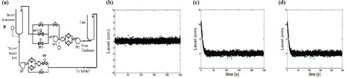
Pietrykowski, Guo, and Smidts (2013) designed a distributed test facility to reproduce BWR conditions, and used a PI controller to control the facility (Figure 17(a)). A steam pump (SP) and a steam valve (SV) are used to control the rate of water represented by a ‘steam liquid exit’. SP speed is constant to create adequate pressure; SV is controlled by the PI controller. The thermal power of the reactor (simulated core) is attached to a steam generator. The full power level is 3350 MWt in this scenario. The rate of water flowing into the steam generator is controlled by an auxiliary feed pump (FP1), a main feed pump (FP2), a main feed valve (MFV), and a bypass feed valve (BFV). The MFV is controlled by a PI controller. By forcing the MFV or SV open, transients are generated, which cause increase or decrease the water level in the SG. In simulations in which the initial water level was in a steady state (Figure 17(b)), the PI controller quickly adjusted transients back to the steady state (Figure 17(c) and 17(d)).

Figure 17. Distributed test facility, and simulation results (Pietrykowski et al., 2013). In these results, the difference from the corresponding steady state are shown; hence all the values are zeroes during the steady state. (a) Steam generator level controller, (b) water level during the steady state, (c) water level after feed water transient and (d) water level after steam transient.

5.4. Fuzzy-PID control for a pebble bed reactor

A reactor can be modelled using a linear system approach. When it is represented as a linear system, it should be expressed by using a transfer function, or by using a look-up table to express the non-linearities in the system. Badgujar, Satpute, Revankar, Lee, and Kim (2012) have investigated a fuzzy-PID controller (Figure 18) for HTPBR, and obtained a linearized model of the HTPBR at different operating powers. The following equations were used to account for feedback reactivity with a homogenized pebble bed reactor core: (5) (6) (7) (8) (9) (10) (11)

Figure 18. HTPBR control. (a) Kinetic model for HTPBR and (b) PID controller.

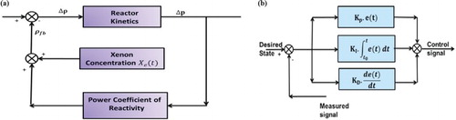
where is the controller output (cm/s), is the reactivity worth () of the control rod per unit length and is dependent on position of control rod in the core, is the dynamic power coefficient of reactivity),is the internal feedback reactivity due to change in power in , is the static power coefficient, is a time-delay constant to account for the reactivity change (s). I is the Iodine concentration (), X is the Xenon concentration (), is the macroscopic fission cross-section of fuel (), is the macroscopic absorption cross-section of Xenon (), is the space-averaged flux (), is the internal feedback reactivity due to Xenon in , is the fuel temperature (K), T_g,ij is the coolant temperature (K), h is the heat transfer coefficient between the fuel and coolant (W/cm²K), and A is the heat transfer area (cm²). The reactor kinetics model was developed and efforts were made to account for Xenon reactivity and the power coefficient of reactivity. In analysis, five power ratings of 100%, 80%, 60%, 40%, and 20% of the rated power were considered. Transfer functions of the reactor at these ratings in the Laplace domain were

For 100% rated power, (12)

For 80% rated power, (13)

For 60% rated power, (14)

For 40% rated power, (15)

For 20% rated power, (16)

Corresponding to these five demands of power, five PID controllers with different sets of PID gains were designed. The five sets of PID gains are represented as Gaussian membership functions (Figure 19). The fuzzy sets for are represented as Gaussian membership functions because they vary nonlinearly and smoothly. This fuzzy logic system uses five rules (Table 4); each consists of an antecedent (‘if’ part) and consequent (‘then’ part). These rules determine the membership of the variables, .

Figure 19. Gaussian membership functions for the gains (a) Membership functions for K_p, (b) membership functions for K_i and (c) membership functions for K_d.

Table 4. Fuzzy rules.

	Antecedent	Consequent
Rule	power

The fuzzy inference processes take into account input Membership functions, Logical operations, Rules to generate aggregation of consequents across the rules, and Defuzzification to generate output. The centroid method is used to generate output from the aggregate output fuzzy set. The generalized expression for the centroid method is as follows (Mendel, 2001), (17)

5.5. Receding horizon control for a steam generator and advanced high-temperature prismatic reactor core

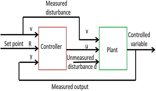
A Receding Horizon Controller (RHC) has been used to control industrial processes (Clarke & Scattolini, 1991; Garcia, Prett, & Morari, 1989; Kothare, Balakrishnan, & Morari, 1996; Kwon & Pearson, 1977; Lee, Kwon, & Choi, 1998; Lee, Kwon, & Lee, 1997; Richalet, Rault, Testud, & Papon, 1978). The behaviour of the process over P future samples is predicted at the current time instant k. The changes in the control variable are predicted to yield the required characteristics in the response of the process. The controller applies only the first computed change in the control variable (Figure 20(a) and 20(b)). This approach offers many advantages over conventional horizon control because of the finite size of the prediction window. This approach is also useful for time-varying systems. This controller has been used to control the water level of a steam generator in PWRs (Lee, Oh, Chun, & Kim, 2012; Na et al., 2005). Irving, Miossec, and Tassart (1980) have obtained the Laplace transfer function for the steam generator, for which RHC is designed.

Figure 20. Output, reference, and control input for the controlled system. (a) Reference and output of the plant (Lee et al., 2012) and (b) control signal generated by the controller (Lee et al., 2012).

To provide sufficient cooling to the reactor core, the water level in the nuclear steam generator must be maintained (Figure 21). The fixed PI gain over all power levels does not work satisfactorily in a steam generator; therefore an RHC has been coupled with a steam generator (Figure 22). In these investigations, the parameters of the system (steam generator) vary with changes in the reactor power; so both linear and non-linear models of the plant were created.

Figure 21. Schematic for the steam generator of a PWR (Kavaklioglu, 2014).

Figure 22. RHC for maintaining the water level.

In the RHC technique, the M current and future control samples are used to predict the future behaviour of the output process over a horizon of P such that P > M. The control moves are chosen so that a quadrature objective function is minimized. Out of M control moves, only the first one is used. After using the first control move, the new values of the measured output variable are obtained. The control window is then moved one step forward and the algorithm is repeated.

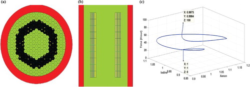
Moreover, the receding horizon control algorithms have been used to control Xenon oscillations in the Advanced High-Temperature Prismatic Reactor (AHTPR) (Badgujar & Park, 2016) (Figure 23).

Figure 23. AHTPR model and controlled Xenon oscillation. (a) Horizontal cross-section of AHTPR625, (b) vertical cross-section of AHTPR625 and (c) controlled oscillations of Xenon and Iodine after external perturbation in upper half of AHTPR625.

In these types of problems, the following type of discretised state-space modelling approach is used. (18) where x(k) is the state vector, is the manipulated control input, v(k) is the measurable disturbance; [A,B,C,E] are coefficient matrices. The output y is dependent on the state variable . For the optimization problem with finite state horizon and finite input horizon, W. H. Kwon and A. E. Pearson have guaranteed close loop stability (Kwon & Pearson, 1978; Lee et al., 1997).

5.6. Genetic-based model predictive control for APR

A genetic-based controller has been used for load following the operation of the APR+ nuclear plant (Lee et al., 2012; Na & Hwang, 2006). The future output required in an optimization problem is predicted by the support vector regression (SVR) model (Figure 24). In PWRs, the power is controlled by movement of the control ‘rods’ and chemical shim over the lifetime of the reactor. Control rods are mainly used to provide reactivity for the shutshown of the reactor and to overcome reactivity changes induced by temperature changes. However, the reactor power can be also controlled by using boric acid (chemical shim control), because Boron is a strong neutron absorber. In daily load following operation of the reactor, the concentration of the Xenon byproduct changes slowly. In this analysis, the control banks, part-strength control banks together with an adjustment of the boric acid concentration are used to control the power level and ASI.

Figure 24. MPC in the form of the GA and SVR algorithm.

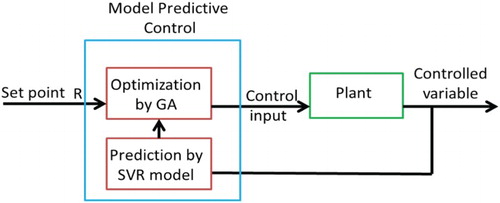
The RHC approach was used, so the future behaviour of the process output was predicted over the prediction horizon P (Figure 20). Only the first control move is applied to obtain the new response of the system. The new measurements are taken to compensate for unmeasured disturbance and model inaccuracies which cause the predicted output to deviate from the measured output. A quadratic function is used as the performance measure, with the following constraints (19) (20) (21) over the control signal. and are, respectively, the minimum and maximum control inputs, and and are, respectively, the minimum and maximum allowable control moves at every time instant. A Kernel function is used to generate the weight of the artificial neural network (ANN) by solving the no-convex unconstrained minimization problem.

The advantage of a genetic algorithm (GA) is that it initiates the search from many points simultaneously rather than from a single point like other conventional methods. Thus, GA can climb up many local maxima simultaneously and therefore is likely to find the global maximum rather than a local one (Goldberg, 1989; Mitchell, 1996). The disadvantage of GAs is that they have high time complexity. In a GA, the candidate solution to the optimization problem is known as a chromosome. GA applies selection, crossover, and mutation operations over the chromosomes to generate a pool of new chromosomes or solutions as illustrated below, with control input u with M moves fitted in a single chromosome: (22) where g = 1,2, … G and G is the total number of chromosomes. Defining crossover probability as and mutation probability as , the GA proceeds in the following steps:

Step 1: Generate G chromosomes with M moves (number of current and future samples of control input). Set iteration counter to n = 1.

Step 2: Evaluate the fitness of all chromosomes. Because the objective function is to be minimized, the reciprocal is used to calculate the total fitness of the population: (23) where is the objective function of the chromosome. The normalized fitness of each chromosome is given by

Step 3: For g = 1 to G, calculate the cumulative probability . Generate a random number 0 ≤ r₁ ≤ 1. Select the chromosome for which . At this point, select a new population of chromosomes. The chance that a chromosome is selected increases its fitness value.

Step 4: Generate another random number 0 ≤ r₂ ≤ 1. If r₂ < P_c then perform the crossover process on the chromosomes, otherwise do not. Choose the crossover site by choosing a random number 0 ≤ r₃ ≤ M−1. Perform a crossover (Table 5).

Table 5. Crossover on control inputs.

Before crossover
After crossover

Step 5: Generate another random number r₄. If r₄ is less than mutation probability P_m, then mutate the selected member. Generally, P_m ≈ 0.01; select a random binary number r_b; use it to determine the way in which a mutation will occur: (24) (25) here random number r lies between 0 and 1. The number of iterations performed and the expected final number of iterations are denoted by iter and itermax, respectively. and are the upper and lower bounds on the kth sample of the control input.

Step 6: Increase the iteration counter by 1, that is, n = n + 1, and return to Step 2.

If the maximum allowed time is expired then stop the iterations and select the chromosome having the lowest objective value.

The Korean Atomic Energy Research Institute (KAERI) has built its own code which is coupled with MATLAB to accomplish these simulations (Cho, Joo, Cho, & Zee, 2002). The code has the following features:

• The depletion problem

• Fuel pin power and pin burnup

• Xenon dynamics

• Adjoint flux determination

• Three-dimensional power shape matching

• In-core and ex-core detector signal evaluation

• Thermal hydraulics (T/H) and design-specific activities including fuel management.

The proposed control algorithm by KAERI has been developed in MATLAB and Visual C++.

5.7. Coordination control for marine NPP

Compared with commercialized NPPs Indian Arihant-class submarine power plants have a smaller core and steam generator, faster response, and stronger load following capacity. Some other researchers, Ping et al., used simulations to investigate the development of control systems for marine NPPs (Ping, Zhao, & Yun, 2012). Generally, systems are designed according to the primary circuits with the assumption of a steady state, that is, the average temperature and inlet temperatures of the coolant and fuel are constant; however, a marine NPP also requires constant pressure of the primary and secondary circuits; so design of the control system is a complex process (Peng, 2005; Peng & Ze, 2001). This work focused on the three control subsystems: (1) Control rod adjustment system including the neutronic model (2) Feedwater control system for the once-through steam generator (OTSG), thermal-hydraulic models of OTSG, turbine valve control systems, and (3) Speed control system of the feedwater pump. The simulation results show that to improve the dynamic characteristic of the system, the pump efficiency must be enhanced.

5.8. Simulations for control of load on the secondary side

5.8.1. Turbine control for electricity generation

Dulau et al. developed a model that uses a PI controller to control the speed of a steam turbine (Dulau & Bica, 2014; Xia, Su, & Zhang, 2008). The design of the gas turbine used in the Brayton cycle is different from the steam turbine. Heng Xie has developed a control system model for the transient behaviour of the gas turbine modular helium reactor (GT-MHR) gas turbine (2011) as follows. The one-dimensional model is used for flow-paths, and the turbine and compressor are considered to be zero-dimensional (Figure 25). The following mass, momentum, and energy equation are used for each component.

Figure 25. GT-MHR module (Xie, 2011).

Mass equation: (26) Momentum equation: (27) Energy equation: (28) where V is the volume (m³), is the density (kg/m³), G is the mass flow rate (kg/s), u is (m/s), velocity (m/s), A is the cross-section area (m²), F is the force (N), h is the enthalpy (J/kg), Q is the heat flow of fluid into the component (Wt), and W is the work done (Wt).

5.8.2. Hydrogen production control

Hydrogen is an environmentally benign fuel that has the potential to replace fossil fuel due to high heat of combustion, but at present Hydrogen production uses fossil fuels. Also, Hydrogen production with direct splitting of water requires a temperature >2500°C. There are several methods for Nuclear-based Hydrogen production. Here, the following two methods are discussed.

(a) the Sulphur–Iodine (SI) process and

(b) the High-temperature electrolysis (HTE) process.

(a) the SI process: The SI cycle is a pragmatic solution for hydrogen production. Some conceptual studies of nuclear-based Hydrogen production to harness Hydrogen energy have been performed by Badgujar (2013). The Hydrogen production plant acts as a heat sink when coupled with a nuclear reactor (Figure 26, Table 6).

Figure 26. Schematic of hydrogen production plant.

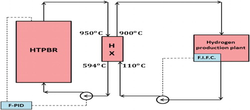
Table 6. Specification for the hydrogen production plant.

Specification	Value
Heat exchanger inlet/outlet temperature at primary (°C)	950/594
Heat exchanger inlet/outlet temperature at secondary (°C)	110/900
Mass flow rate in primary/secondary (kg/s)	135.22/60.74
Reactor power (MWt)	250
Hydrogen production (mole/s)	416

The plant is only used for Hydrogen production, so active components are powered by an external electric supply.

The SI cycle is completed in three steps. Each step is accomplished in one of the sections (Figure 27).

Figure 27. Representation of the SI cycle (Brown et al., 2002).

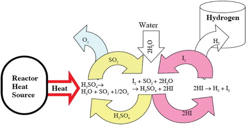
Section 1: SO₂ + I₂ + 2H₂O → 2HI + H₂SO₄ (∼100°C); this is called the Bunsen reaction. Section 2: H₂SO₄ → SO₂ + H₂O + O₂ (900°C); the SO₂ product is recycled back to Section 1.

Section 3: 2HI → H₂ + I₂ (500°C). The product H₂ is stored; the I₂ is recycled back to Section 1.

After storing the product H_2, the SO₂ and I₂ are recycled. Most of the energy required for Hydrogen production is consumed by the SA and HI decomposer (Table 7). The flowsheet described in Lee (2008) for Hydrogen production was scaled up linearly by a factor of 416 to produce Hydrogen at the rate of 416 mole/s. At this rate, the requirement of thermal power on the primary of heat exchanger is 249.184 MWt; hence the reactor model is designed to provide 250 MWt power to provide sufficient thermal energy.

Table 7. Energy requirement in KJ/mol.

Energy requirement	Energy
Section 2	411∼420
Section 3	167
Pumping	17

The valve position is controlled by a Flow indicator and Fuzzy Controller (FIFC) with five rules (Table 8).

Table 8. Fuzzy rules used to control Hydrogen production.

Rule	H2 production rate	Valve position

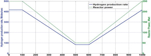
The hydrogen production rate varies with the reactor power (Figure 28). The thermal efficiency can be > 60% when parameters are optimized.

Figure 28. Hydrogen production rate (mole/s) with reactor power (MWt) against time (Badgujar, 2013).

(b) HTE process:

The chemical reactions that take place in HTE are as follows, NET reaction: H₂O→H₂ + 0.5O₂.

These reactions are illustrated in Figure 29 with the electrolysis cell as follows.

Figure 29. Unit cell for electrolysis.

In HTE, steam is decomposed at a high temperature of around 900°C. On the bench scale, a test has been carried out by INL, JAERI to investigate electrolysis characteristics for 1000 h (Hino & Miyamoto, 2004; O’Brien et al., 2009).

The working principal of the electrolysis is shown in Figure 29. Steam is dissociated by an electron supplied externally by a DC supply on the surface of the cathode. Hydrogen molecules are formed on the surface of the cathode, while oxygen ions are diffused through electrolyte and form oxygen molecules on the surface of the anode by releasing electrons. The hydrogen produced in this process has high purity. The combination of a high-efficiency power cycle with VHTR and the direct utilization of nuclear process heat can provide thermal-to-hydrogen conversion efficiency of 50% or higher.

Long-term degradation in a unit cell is caused by the degradation of the electrodes, the electrolyte, or electrode-electrolyte delamination. For a stack of 25 cells the area-specific resistance (ASR) increases ∼0.6 to 1.33 Ω cm². This is certainly an unacceptable rate of degradation beyond 1000 h. In the HTE process, there are material issues such as corrosion and degradation, issues related with hydrogen leakage rather than control issues for sustainable hydrogen production.

It should be noted that in both of these methods of hydrogen production, one of the safety issues is the migration of tritium produced in the core to the downstream process (product hydrogen). Tritium is produced through ternary fission reaction of the fuel and neutron capture reactions of Li-6, Li-7, B-10 present in the graphite and burnable poison and He-3 in the coolant. This safety concern can be overcome by isolating primary and secondary circuits with the help of an intermediate heat exchanger.

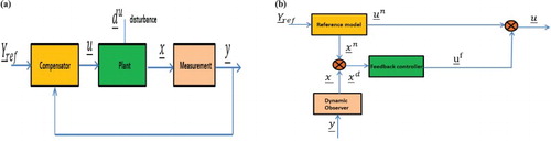
5.9. Feedforward and feedback control

Application of the Non-Linear Space-Time Nuclear Reactor Control algorithm was demonstrated on a Canadian Deutrium Natural Uranium (CANDU) reactor (Yorke & Cherchas, 1981). In this reactor, spent fuel is replaced using an on-line refuelling machine, which thereby enables control of long-term power distribution. Therefore, consideration of space-time reactor control is an important aspect of the CANDU system design. In this work, the state variables are distinguished as either directly controlled (d) or non-directly controlled (n) state variables. Neutron density is directly controlled (recognized as vector ) and amplitudes for delayed neutron precursor C(t), densities of Iodine I(t) and Xenon X(t), temperatures of the fuel T_J(t), coolant T_C(t), boiler inlet T_Bi(t), and reactor inlet coolant T_ci(t) (recognized as vector ) are indirectly controlled. The state vector is expressed as . The control input is a summation of feedforward and feedback control input (Figure 30(a) and 30(b)).

Figure 30. Control for CANDU reactor. (a) Feedback and feedforward controller for a CANDU reactor and (b) control signal.

5.10. Neural network control for PWR

Online supervision of plant condition during reactor operation is one of the most important tasks for an NPP to ensure operational safety and maintenance. Nabeshima, Inoue, Kudo, and Suzuki (2000), Nabeshima, Suzudo, Ohno, and Kudo (2002) have attempted to solve this problem. Conventionally, the fault threshold levels for each plant parameter are set and an alert signal is generated as soon as the monitored signal exceeds a predetermined or threshold level. Nonetheless, in many cases, when an anomaly is detected, it may be too developed to undo. Hence, a model-based method is used, which is better for early fault detection than are the conventional threshold level-based systems. One of the advantages of a neural network is its ability to model multi-output process systems from measurement information without using physical expressions. Therefore, neural networks can be beneficial in monitoring of nuclear reactors, in addition to other applications (Uhrig, 1991). The 22 most significant plant signals are used for plant modelling by the neural network controller. A hybrid reactor monitoring system that is a combination of a neural network and a rule-based real-time expert system has been successfully tested using the online PWR simulator.

5.11. Neural network for an accelerator-driven system

Zio, Broggi, and Pedroni (2009) used a Causal Recursive Back-Propagation algorithm to train on-line an Infinite Impulse Response–Locally Recurrent Neural Network (IIR–LRNN) to model the dynamics of an accelerator-driven system. ANNs can learn input–output relationships that are non-linear by a process of training on many different input/output sets, some of which can be noisy, incomplete, and even contradictory, but the commonly used feedforward ANN has capability to model static input–output mappings. Theses on neural networks cannot reproduce the behaviour of dynamic systems (Rumelhart, Hinton, & Williams, 1986). Currently, dynamic recurrent neural networks (RNNs), especially IIR–LRNNs, are attracting attention because of their potential to provide accurate approximations to the dynamic behaviour of non-linear systems.

5.12. Linear regulator with optimal control for a PHWR

A simulation for a near-optimal linear regulator has been designed to control Xenon-induced oscillations (Tiwari, Bandyopadhyay, & Govindarajan, 1996). It uses optimal control theory (Kirk, 1970; Sage, 1968). The neutronics of a large nuclear plant is loosely coupled; that is, change in flux at a point of the core will not instantaneously affect other points in the reactor. Also, Xenon poisoning can generate a serious situation of flux tilting. Because both fast and slow dynamic phenomena occur in the reactor, system representation with state variables causes stiffness and ill-conditioning, so optimal control for such a high-order model is not practical. A nodal model or a quasi-static model is designed by dividing the reactor core into fourteen zones in each of which material composition and flux are considered constant (Duderstadt & Hamilton, 1976; Stacey, 1969). The mathematical model of the reactor is non-linear and uses 56 states with 14 inputs to account for the Xenon–Iodine dynamics. The 56-state variable model is decomposed into a 42nd-order slow subsystem and a 14th-order fast subsystem. The problem of regulating the slow subsystem is designed as a cheap control problem to regulate a 28th-order sub-model and a 14th-order sub-model. The 14th-order fast subsystem regulator problem is also solved. This method is adopted to solve the control problem for a PHWR but it accounts only for Xenon poisoning and neglects other vital feedback. The following equations give a performance index to be minimized, and optimal control input for a system represented by a state-space representation of the reactor model: (29) where S is the solution of the Riccati equation, matrix B is from the state-space representation of the system with state vector z, Q and R are weighing matrices, and is the reactivity input. This approach ignores other vital feedback.

5.13. Linear regulator with optimal control for a PWR

A system to control reactor power should satisfy three requirements: (i) It should operate safely and reliably; (ii) It should maintain maximum power output of the reactor; and (iii) It should possess a certain stability margin, suitable peak overshoot, and transient time. Zarabadipourand and Emadi (2011) have used a balancing approximation method to reduce the order of the reactor model, and further designed an observer-controller for a reactor power control system. The simplified reactor power consists of point kinetics equations with six groups of delayed neutrons and two thermal feedback arising from changes in fuel temperature and coolant temperature. The core heat transfer is modelled as one fuel node and two coolant nodes. The simulations results satisfy above three requirements. Parameters of a Three-Mile Island-type PWR reactor were used for simulation; the performance index, and optimal control input for this system are given as (30) The value 200 was chosen to account for the fast speed of control rod . For this cost function, when the reactor power deviates, the penalty on the deviation of fuel temperature from its equilibrium value is reduced, but the penalties on coolant exit temperature deviations and control rod speed are increased (Chenand & Zhang, 2009). Alibeik and Setayeshi (2003), Arab-Alibeik and Setayeshi (2003) solved an adaptive-cost-function optimal controller design for a PWR nuclear reactor. The disadvantage of these modelling techniques is that they are based on point kinetics approximation; therefore, Li (2014) developed a two-point-based model for a PWR core. In this model, the core is divided into two equal halves (bottom and top), which are treated as points and connected by the neutron diffusion coefficient (Dong, Huang, & Zhang, 2010).

5.14. Neural network and fuzzy control for VVER

Considering the non-linearity of local power peaking of the core and safety margins for fuel temperature, controlling the nuclear reactor core during load following operation encounters some difficulties. Boroushaki, Ghofrani, Lucas, & Yazdanpanah, (2003a, 2003b) investigated ways to use an RNN and fuzzy system to identify and control a Vodo-Vodyanoi Energetichesky Reaktor (VVER) Nuclear Reactor core. A VVER type reactor core is represented by a multi-non-linear autoregressive structure with exogenous inputs (NARX), including neural networks that are trained by a heuristic compound learning method. The NARX is trained by an accurate three-dimensional (3D) core calculation code DYNCO. An intelligent nuclear reactor core controller can use the NARX neural network to generate data quickly. The controller also uses a fuzzy system that expresses the operator’s knowledge and experience in the decision-making process. The simulation results using DYNCO proves that the proposed controller can control the reactor core well during load following operations by manoeuvring groups of control rods optimally and by using a variable overlapping strategy. NARX with gradient-descent learning converges quickly and its generalization ability is better than those of recurrent multilayer perceptron (RMLP) (Lin, Horne, Tino, & Giles, 1996). This intelligent core controller model mainly includes

1. The NARX core model

2. Control Rod Group (CRG) manoeuvre generator

3. A fuzzy critic and an optimum CRGs manoeuvre finder.

To capture any process dynamics that is not included in the training set, NARX is updated with real plant data at any time interval. The fuzzy critic considers all possible CRG manoeuvres and generates the optimal CRG manoeuvres that overlap for the next time interval.

5.15. Linear fractional transformation-based control for a training, research, isotopes, general atomics (TRIGA) research reactor

For the Penn State TRIGA research reactor, a robust control design procedure for a nuclear reactor has been developed and experimentally validated (Shaffer, Edwards, & Lee, 2005). The robust controller has been used as a component of an autonomous control system. For a robust control design, two methods of specifying a low-order (fourth-order) nominal-plant model have been used: (1) by approximation based on the ‘physics’ of the process (one-effective-delayed-group point kinetics) and (2) by an optimal Hankel approximation of a higher-order plant model. To demonstrate control techniques for nuclear reactors, non-linear point kinetics models of a reactor along with two temperature feedback are used. The performance objective is chosen to minimize tracking error and control energy. The controller obtained using the optimal Hankel approximation has improved performance because under ideal conditions it has a marginally faster settling time than the controller derived using the one-group prompt-jump approximation. Nonetheless, when the two methods were compared experimentally on the TRIGA reactor these differences could not be noticed because of measurement noise (Shaffer, He, & Edwards, 2004).

5.16. Optimal control for a research reactor

Another optimal power control system design for a research nuclear reactor has been investigated by Zhao, Cheung, and Yeung (2002) to improve the desired performance over the conventional controller. To obtain the desired performance of the control system, an objective function or quadratic performance function is selected, in the time domain. Some of the parameters for the open loop transfer function were taken from Zhou (1990). This objective function is converted to the frequency domain by applying Paserval’s theorem. The optimal transfer function can be found by solving the problem in the frequency domain. With the application of the state feedback theory, the transfer function of the nuclear reactor control system is deduced to optimize the transfer function. In simulations the performance of the control system was improved; therefore the method presented is useful.

5.17. Sliding mode control for an AHWR

Bandyopadhyay, Alemayehu, Abera, and Janardhanan (2006) presented the design of sliding mode control for a higher-order system with a reduced order model. The reduced order model produces similar performance to that of the higher-order system. A switching surface s(k) = 0 is used to represent a desired system dynamics which has lower order than the given plant. A suitable control is obtained such that any state of the system outside the switching surface is forced to reach the surface in finite time. The sliding mode motion for the high-order system is generated when a sliding mode control is designed from the reduced order model and applied to the higher-order system by aggregation. Munje, Patre, Shimjith, and Tiwari (2013) considered a 90th-order model with 5 inputs and 18 outputs for an AHWR. In this work, the numerically ill-conditioned system of the AHWR was split into a 73rd-order ‘slow’ subsystem and a 17th-order ‘fast’ subsystem. The sliding mode controller was designed from the slow subsystem. Additionally, by using simple linear transformation matrices, a sliding mode controller for the full system was generated.

5.18. Autonomous control for space reactor systems

Upadhyaya et al. investigated the Autonomous Control of Space Reactor Systems. Generating a stable control in different operation modes to ensure stable transition between them is a necessary requirement of a space reactor control system. The main operating modes required for a space reactor are normal operation at different power levels, hot standby mode for system testing, scheduled mission task, transition to long-term shutdown, and cold shutdown mode for maintenance purposes. The two major transitional modes are start-up and shutdown. The reactor systems and equipment must be monitored vigilantly and controlled to guarantee compliance with safety requirements when operated in transitional modes. The space reactor control system must give the operator the capability to monitor and optimize performance and health to back up the mission for extended operation. The reactor system is anticipated to operate continuously, remotely, and independently for up to 15 years in deep-space missions because during such prolonged operation, many thermal and electric components may degrade significantly. Also, different models should be automatically updated after an interval of a minute. The model predictive controller with dynamic optimization can be implemented on the same time scale during space reactor power operation. A lumped parameter simulation model is used for the thermo-electric SP-100 reactor having a fast spectrum. It is a lithium-cooled fuel pin reactor from which waste heat is dissipated through a heat pipe distribution system and space radiators (Seo, 1986). Adaptive state estimation has been performed using a Kalman filter.

5.19. Control for a Tehran research reactor with the power probability density function

By controlling the mean and variance of the output, the stochastic system can be controlled. The algorithm is executed with the guess that the output of the system obeys the Gaussian distribution. This guess is true for many systems. Bounded output distribution control theory has been proposed (Wang & Yue, 2003) to control the output probability density function (PDF) instead of the mean or variance of the system output. B-spline functions have been used to model the reactor PDF (Abhariana & Fadaei, 2014), and the power controller is designed based on an approximation model. The modelling, controller design, and performance assessment method have been used to control the power of the Tehran research reactor. The performance assessment index is a tracing error index (31) where f is the PDF of the reactor power, g is the PDF of the specified and desired power. Particle swarm optimization (PSO) has been used to solve the control law (Kennedy & Eberhart, 1995).

5.20. control application

Naidu, Charalambous, Moore, and Abdelrahma (1994) provided controller design methods that use the two-step method and Riccati equation approach, but Dong and Yang (2008) proposed a new controller design method in terms of solutions to linear matrix inequalities (LMIs) that eliminated regularity restrictions connected to the Riccati-based solution. A method to determine the upper bound of a singular perturbation parameter has been also established to satisfy the given performance bound requirement. The problem of control synthesis for fast sampling discrete-time singularly perturbed systems is illustrated with a numerical example. Upper bounds on a singular perturbation parameter were determined for the nuclear reactor problem.

5.21. Takagi–Sugeno control application

An improved L2 gain controller synthesis for a Takagi–Sugeno fuzzy system has been investigated by Xie (2008). The L₂ gain performance criterion (Jadbabaie, 1999; Li, Wang, Niemann, & Tanaka, 2000) can be used to assess the control system performance such as external disturbance rejection, robust stability, or performance analysis towards the modelling errors, structured or unstructured parameter uncertainty, just like control performance criteria. Xie W. has developed a T–S fuzzy controller with a three-step procedure. First, a new T–S fuzzy model structure was developed; it was composed of the original T–S fuzzy plant plus stable pre- and post-filters on the input and the output of the T–S fuzzy plant. Second, an L2-gain performance controller with the LMI optimal technique for this augmented T–S fuzzy model was designed. The L2 gain performance of the T–S fuzzy controller can be reduced because the input and the output matrices of this augmented T–S fuzzy model are not dependent on the membership functions of the premise variables. In the third step, an augmented controller (composed of the controller obtained from step two and stable pre- and post-filters) with improved L2 gain performance was obtained. Badgujar, Lemma, and Won (2015) have attempted to combine the Takagi–Sugeno Neuro-Fuzzy controller with a conventional PID controller.

6. Conclusion

Some basics about nuclear fission and the dependence of reactor power on various parameters were explained. A comprehensive review for various control problems in nuclear reactors with different types of loads is presented. The causes of reactivity change have been described, and reactivity feedback arising from various parameters are considered. The causes of Xenon oscillation are discussed. In the first part, the architectures for hardware of I&C were reviewed; in the second part, simulation techniques used in the practices were explained. Various control algorithms are considered and elaborated. The controls aspects while coupling the reactor core with different types of the loads were explained.

Depending upon the complexity of the system, certain algorithms can be chosen. Determining the transfer function and designing the robust control is convenient for a system with few state variables. But this frequency-based approach cannot be generalized for systems having several state variables. Other model-based control algorithms can be designed and their performance costs can be compared while selecting the algorithm.

Acknowledgements

The author would like to thank the Division of Advanced Nuclear Engineering, POSTECH. The author would like to express gratitude to the distinguished professor and Editor-in-chief Zidong Wang from Brunel University, UK. Thanks are extended to unknown reviewers for their valuable comments to enhance the quality of this article.

Disclosure statement

The authors declare that there is no conflict of interests regarding the publication of this paper.

ORCiD

Kushal  D.  Badgujar http://orcid.org/0000-0003-2160-4447

Additional information

Funding

This work was supported by the World Class University program through the National Research Foundation of Korea funded by the Ministry of Education, Science and Technology [R31-30005]. Currently, the research is supported by BK21+ program through the National Research Foundation of Korea funded by the Ministry of Education, Science and Technology.

References

- Abhariana, A. E., & Fadaei, A. H. (2014). Power probability density function control and performance assessment of a nuclear research reactor. Annals of Nuclear Energy, 64, 11–20. doi: 10.1016/j.anucene.2013.09.018
- Ablay, G. (2013). A modeling and control approach to advanced nuclear power plants with gas turbines. Energy Conversion and Management, 76, 899–909. doi: 10.1016/j.enconman.2013.08.048
- Akin, H. L., & Altin, V. (1991). Rule-based fuzzy logic controller for a PWR-type nuclear power plant. IEEE Transactions on Nuclear Science, 38(2), 883–890. doi: 10.1109/23.289405
- Alibeik, H. A., & Setayeshi, S. (2003). Improved temperature control of a PWR nuclear reactor using an LQG/LTR based controller. IEEE Transactions on Nuclear Science, 50(1), 211–218. doi: 10.1109/TNS.2002.807860
- Arab-Alibeik, H., & Setayeshi, S. (2003). An adaptive-cost function optimal controller design for a PWR nuclear reactor. Annals of Nuclear Energy, 30(6), 739–754. doi: 10.1016/S0306-4549(02)00116-0
- Badgujar, K. D. (2013). Design of fuzzy-pid controller for hydrogen production using HTPBR. Proceedings of the 21st ICONEPOWER2013, ICONE21-15037. Chengdu, China.
- Badgujar, K. D., Lemma, W. M., & Won, S. C. (2015). Adaptive neuro-fuzzy controller for high temperature gas cooled reactor. International Journal of Soft Computing and Engineering, 5(1), 69–75.
- Badgujar, K. D., & Park, P. G. (2016). Modelling and control for eliminating flux oscillations in generation IV high temperature gas cooled reactor. IET, 52(3), 190–192.
- Badgujar, K. D., Satpute, S. R., Revankar, S. T., Lee, J. C., & Kim, M. H. (2012, October 25–26). Design of fuzzy-PID controller for high temperature pebble bed reactor. Proceedings of the Transactions of the Korean Nuclear Society Autumn Meeting, Gyeongju, South Korea.
- Badgujar, K. D., Singh, O. P., Singh, S., & Revankar, S. T. (2012, July 30–August 3). Power coefficient of reactivity determination for HTPBR and its application for reactivity initiated transients. Proceedings of the 20th ICONE POWER2012, ICONE20POWER2012-55058, Anaheim, California, USA.
- Bandyopadhyay, B., Alemayehu, G., Abera, E., & Janardhanan, S. (2006). Sliding mode control design via reduced order model. Proceedings of the IEEE ICIC 2006, International Conference, Industrial Technology, 2006 (pp. 1538−1541). Mumbai, India.
- Bel, G. I., & Glasstone, S. (1970). Nuclear reactor theory. New York: Van Nostrand Reinhold.
- Boroushaki, M., Ghofrani, M. B., Lucas, C., & Yazdanpanah, M. J. (2003a). Identification and control of a nuclear reactor core (VVER) using recurrent neural networks and fuzzy systems. IEEE Transactions on Nuclear Science, 50(1), 159–174. doi: 10.1109/TNS.2002.807856
- Boroushaki, M., Ghofrani, M. B., Lucas, C., & Yazdanpanah, M. J. (2003b). An intelligent nuclear reactor core controller for load following operations, using recurrent neural networks and fuzzy systems. Annals of Nuclear Energy, 30(1), 63–80. doi: 10.1016/S0306-4549(02)00047-6
- Brown, L. C., Besenbruch, G. E., Lentsch, R. D., Schultz, K. R., Funk, J. F., Pickard, P. S., … Showalter, S. K. (2002). High efficiency generation of hydrogen fuels using nuclear power (Technical Report, GA–A24285 Rev. 1).
- Chenand, D. K., & Zhang, D. F. (2009). Study on optimal control method for load following operation of nuclear reactors. Proceedings of the Intelligent Computing and Intelligent Systems, 2009, ICIS 2009 (vol. 2, pp. 278−281). Shanghai, China.
- Cho, B. O., Joo, H. G., Cho, J. Y., & Zee, S. Q. (2002, October). MASTER: Reactor core design and analysis code. Proceeding of the 2002 Int. Conf. New Frontiers of Nuclear Technology: Reactor Physics PHYSOR2002, Seoul, Korea.
- Clarke, D. W., & Scattolini, R. (1991). Constrained receding – horizon predictive control. IEE Proceedings D Control Theory and Applications, 138(4), 347–354. doi: 10.1049/ip-d.1991.0047
- Dong, J., & Yang, G. H. (2008). H control for fast sampling discrete-time singularly perturbed systems. Automatica, 44(5), 1385–1393. doi: 10.1016/j.automatica.2007.10.010
- Dong, Z., Huang, X., & Zhang, L. (2010). A nodal dynamic model for control system design and simulation of an MHTGR core. Nuclear Engineering and Design, 240(5), 1251–1261. doi: 10.1016/j.nucengdes.2009.12.032
- Duderstadt, J. J., & Hamilton, L. J. (1976). Nuclear reactor analysis. New York: John Wiley & Sons.
- Dulau, M., & Bica, D. (2014). Simulation of speed steam turbine control system. Procardia Technology, 12, 716–722. doi: 10.1016/j.protcy.2013.12.554
- Garcia, C. E., Prett, D. M., & Morari, M. (1989). Model predictive control: Theory and practice – a survey. Automatica, 25(3), 335–348. doi: 10.1016/0005-1098(89)90002-2
- Glasstone, S., & Sesonski, A. (1963). Nuclear reactor engineering (Vol. 1&2). New York: Van Nostrand Reinhold.
- Goldberg, D. E. (1989). Genetic algorithms in search, optimization, and machine learning. Reading, MA: Addison Wesley.
- Gray, S. F., & Basu, S. (2009, June). Turbine control system upgrade for Bruce nuclear plant units 1 and 2. Proceedings of the Electro/Information Technology, 2009. eit ‘09, IEEE International Conference (pp. 429–436). Windsor, Canada.
- Hashemian, H. M., Morton, G. W., & Shumaker, B. D. (2009, June). Advanced digital rod position indication system for existing and next generation nuclear reactors. Proceedings of the New Nuclear Frontiers, 30th Annual Canadian Nuclear Society Conference and 33rd CNS/CNA Student Conference (pp. 303–315). Calgary, Alberta, Canada: Canadian Nuclear Society.
- Heger, A. S., Alang-Rashid, N. K., & Jamshidi, M. (1995). Application of fuzzy logic in nuclear reactor control part I: An assessment of state-of-the-art. Nuclear Safety, 36(1), 109–121.
- Henry, A. F. (1997). Nuclear reactor analysis. Cambridge: Massachusetts Institute of Technology Press.
- Hetrick, D. L. (1971). Dynamics of nuclear reactors. London: The University of Chicago Press.
- Hino, R., & Miyamoto, Y. (2004). Hydrogen production by high temperature of steam (pp. 119−124). (JAERI Technical Report).
- Irving, E., Miossec, C., & Tassart, J. (1980). Toward efficient full automatic operation of the PWR steam generator with water level adaptive control (pp. 309–329). BNES, London, Boiler Dynamic and Control in Nuclear Power Stations.
- Jadbabaie, A. (1999). A reduction in conservatism in stability and L2 gain analysis of T-S fuzzy systems via linear matrix inequalities. Proceedings of the IFAC14∼ Triennial World Congress (pp. 285–289).
- Kavaklioglu, K. (2014). Support vector regression model based predictive control of waterlevel of U-tube steam generators. Nuclear Engineering and Design, 278, 651–660. doi: 10.1016/j.nucengdes.2014.08.018
- Kenji, M., & Hiroshi, S. (2014). Development and assurance of high integrity of digital I&C systems for Mitsubishi PWR plants. Nuclear Safety and Simulation, 5, 325–331.
- Kennedy, J., & Eberhart, R. C. (1995). Particle swarm optimization. Proceedings of the IEEE Int. Conf. on Neural Networks (pp. 1942–1948). WA, Australia.
- Kinoshita, M., Fukuzaki, T., Stoh, T., & Miyake, M. (1988). An automatic operation method for control rods in BWR plants, in In-Core Instrumentation and Reactor Core Assessment. Proceedings of the Specialists’ Meeting (pp. 213–220). Cadarache, France.
- Kirk, D. E. (1970). Optimal control theory – An introduction. Englewood Cliff, NJ: Prentice Hall.
- Kothare, M. V., Balakrishnan, V., & Morari, M. (1996). Robust constrained model predictive control using linear matrix inequality. Automatica, 32(10), 1361–1379. doi: 10.1016/0005-1098(96)00063-5
- Kuan, C. C., Lin, C., & Hsu, C. C. (1992). Fuzzy logic control of steam generator water level in pressurized water reactors. Nuclear Technology, 100(1), 125–134.
- Kwon, W. H., & Pearson, A. E. (1977). A modified quadratic cost problem and feedback stabilization of a linear system. IEEE Transactions on Automatic Control, 22(5), 838–842. doi: 10.1109/TAC.1977.1101619
- Kwon, W. H., & Pearson, A. E. (1978). On feedback stabilization of time varying discrete linear systems. IEEE Transactions on Automatic Control, 23(3), 479–481. doi: 10.1109/TAC.1978.1101749
- LaBar, M. P. (2002). The Gas Turbine – Modular Helium Reactor: A promising option for near term deployment (Technical Report GA-A23952).
- Lamarsh, J. P. (1966). Introduction to nuclear reactor theory. New York: Addison-Wesley.
- Lee, B. J. (2008). Analysis and optimal process development of iodine-sulfur cycle for nuclear hydrogen production (PhD thesis). Korea Institute of Science and Technology, Daejeon, South Korea.
- Lee, J. C., Jones, K. A., & McCoy, W. I. (1971). Axial stability measurements at the Rochester gas and electric reactor. Transactions of the American. Nuclear Society, 14(Suppl. 2), 15.
- Lee, J. C., & Mc Cormick, N. J. (2011). Risk and safety analysis nuclear systems. New York: John Wiley & Sons.
- Lee, J. W., Kwon, W. H., & Choi, J. (1998). On stability of constrained receding horizon control with finite terminal weighting matrix. Automatica, 34(12), 1607–1612. doi: 10.1016/S0005-1098(98)80015-0
- Lee, J. W., Kwon, W. H., & Lee, J. H. (1997). Receding horizon H tracking control for time-varying discrete linear systems. International Journal of Control, 68(2), 385–400. doi: 10.1080/002071797223686
- Lee, S. W., Kim, J. H., Na, M. G., Kim, D. S., Yu, K. J., & Kim, H. G. (2012). Design of a load following controller for Apr+ nuclear plants. Nuclear Engineering and Technology, 44(4), 369–378. doi: 10.5516/NET.04.2012.509
- Lee, Y. J., Oh, S. J., Chun, W., & Kim, N. J. (2012). The model predictive controller for the feedwater and level control of a nuclear steam generator. Nuclear Engineering and Technology, 44(8), 911–918. doi: 10.5516/NET.04.2012.002
- Lewis, E. E. (1977). Nuclear power reactor safety. New York: John Willey & Sons.
- Li, G. (2014). Modeling and LQG/LTR control for power and axial power difference of load-follow PWR core. Annals of Nuclear Energy, 68, 193–203. doi: 10.1016/j.anucene.2014.01.022
- Li, J., Wang, H. O., Niemann, D., & Tanaka, K. (2000). Dynamic parallel distributed compensation for Takagi-Sugeno fuzzy systems: An LMI approach. Information Sciences, 123(3−4), 201–221. doi: 10.1016/S0020-0255(99)00129-2
- Lin, T., Horne, B. G., Tino, P., & Giles, C. L. (1996). Learning long-term dependencies in NARX recurrent neural networks. IEEE Transactions on Neural Networks, 7, 1329–1338. doi: 10.1109/72.548162
- Mamdani, E. H., & Assilian, S. (1975). An experiment in linguistic synthesis with a fuzzy logic controller. International Journal of Man-Machine Studies, 7(1), 1–13. doi: 10.1016/S0020-7373(75)80002-2
- Mendel, J. M. (2001). Uncertain rule-based fuzzy logic systems: Introduction and new directions. Upper Saddle River, NJ: Prentice Hall PTR.
- Mitchell, M. (1996). An introduction to genetic algorithms. Cambridge: MIT Press.
- Munje, R. K., Patre, B. M., Shimjith, S. R., & Tiwari, A. P. (2013). Sliding mode control for spatial stabilization of advanced heavy water reactor. IEEE Transactions on Nuclear Science, 60(4), 3040–3050. doi: 10.1109/TNS.2013.2264635
- Na, M. G., & Hwang, I. J. (2006). Design of a PWR power controller using model predictive control optimized by a genetic algorithm. Nuclear Engineering and Technology, 38(1), 81–92.
- Na, M. G., Jung, D. W., Shin, S. H., Jang, J. W., Lee, K. B., & Lee, Y. J. (2005). A model predictive controller for load following operation of PWR reactors. IEEE Transactions on Nuclear Science, 52(4), 1009–1020. doi: 10.1109/TNS.2005.852651
- Nabeshima, K., Inoue, K., Kudo, K., & Suzuki, K. (2000). Nuclear power plant monitoring with recurrent neural network. Knowledge-based Intelligent Information and Engineering Systems, 4(4), 208–212.
- Nabeshima, K., Suzudo, T., Ohno, T., & Kudo, K. (2002). Nuclear reactor monitoring with the combination of neural network and expert system. Mathematics and Computers in Simulation, 60(3–5), 233–244. doi: 10.1016/S0378-4754(02)00018-6
- Naidu, D. S., Charalambous, C. D., Moore, K. L., & Abdelrahma, M. A. (1994). H1-optimal control of singularly perturbed discrete-time systems and risk sensitive Control. Proceedings of the 33rd IEEE Conf. Decision and Control (vol. 2, pp. 1706–1711). Lake Buena Vista, Florida.
- Nojiri, N., Shimakawa, S., Fujimoto, N., & Goto, M. (2004). Characteristic test of initial HTTR core. Nuclear Engineering and Design, 233(1–3), 283–290. doi: 10.1016/j.nucengdes.2004.08.015
- O’Brien, J. E., Stoots, C. M., Herring, J. S., Condie, K. G., & Housley, G. K. (2009). The high-temperature electrolysis program at the Idaho national laboratory: Observations on Performance Degradation (INL/CON-09-15564).
- Peng, M. (2005). Research on control strategy of marine PWR nuclear power plant under ideal steady-state programming. Journal of Harbin Engineering University, 26(6), 0–0.
- Peng, M., & Ze, D. (2001). Influence of ideal steady-state programming on collectivity performance of marine PWR NPP. Journal of Harbin Engineering University, 22(1), 16–20.
- Pietrykowski, M., Guo, Q., & Smidts, C. (2013). Network distribution effects on a steam generator level control system. Transactions of the American Nuclear Society, 109(Part 1), 312–315.
- Ping, H., Zhao, F., & Yun, T. (2012). Coordination control and simulation for small nuclear power plant. Progress in Nuclear Energy, 58, 21–26. doi: 10.1016/j.pnucene.2012.02.001
- Reitsma, F., & Naidoo, D. (2003). Evaluating the control rod modelling approach used in the South African PBMR: Comparison of VSOP calculations with ASTRA experiments. Nuclear Engineering and Design, 222(2–3), 147–159. doi: 10.1016/S0029-5493(03)00009-8
- Richalet, J., Rault, A., Testud, J. L., & Papon, J. (1978). Model predictive heuristic control: Applications to industrial processes. Automatica, 14, 413–428. doi: 10.1016/0005-1098(78)90001-8
- Ruan, D., & van der Wal, A. J. (1998). Controlling the power output of a nuclear reactor with fuzzy logic. Information Sciences, 110(3–4), 151–177. doi: 10.1016/S0020-0255(98)10027-0
- Rumelhart, D. E., Hinton, G. E., & Williams, R. J. (1986). Parallel distributed processing: Explorations in the microstructure of cognition, vol. 1: Foundations. (D. E. Rumelhart & J. L. McClelland, Eds.). Cambridge: MIT Press.
- Sage, A. P. (1968). Optimum systems control. Englewood Cliff, NJ: Prentice Hall.
- Schulz, E. J., & Lee, J. C. (1980). Time-optimal control of spatial xenon oscillations to a generalized target. Nuclear Science and Engineering, 73, 140–152.
- Seo, J. T. (1986). SNPSAM-Space Nuclear Power System Analysis Model (MS Thesis). University of New Mexico, Albuquerque.
- Shaffer, R. A., He, W., & Edwards, R. M. (2004). Design and validation of optimized feedforward with robust feedback control of a nuclear reactor. NuclearTechnology, 147(2), 240–257.
- Shaffer, R. A., Edwards, R. M., & Lee, K. Y. (2005). Design and validation of robust and autonomous control for nuclear reactors. Nuclear Engineering and Technology, 37(2), 139–150.
- Smith, C. W., & Mathie, F. (1973). Computer-controlled refueling machine at Fort St.Vrain. IEEE Transactions on Nuclear Science, 20(1), 780–785. doi: 10.1109/TNS.1973.4326998
- Stacey, W. M., Jr. (1969). Space time nuclear reactor kinetics. New York, NY: Academic Press.
- Suzuki, N., & Shimazu, Y. (2008). Reactivity-initiated-accident analysis without scram of a molten salt reactor. Journal of Nuclear Science and Technology, 45, 575–581. doi: 10.1080/18811248.2008.9711881
- Tertmuma, S., Kishiwada, K., Takahashi, H., Iijima, T., & Hayashi, H. (1988). Application of fuzzy algorithms for the feedwater control system in Fugen HWR. Proceedings of the International Conference on Man-Machine Interface in the Nuclear industry (pp. 463–473).
- Tiwari, A. P., Bandyopadhyay, B., & Govindarajan, G. (1996). Spatial control of a large pressurized heavy water reactor. IEEE Transactions on Nuclear Science, 43(4), 2440–2453. doi: 10.1109/23.531794
- Uhrig, R. E. (1991). Potential application of neural networks to the operation of nuclear power plants. Nuclear Safety, 32(1), 68–79.
- Upadhyaya, B. R., Zhao, K., Perillo, S. R. P., & Xu, X. Autonomous Control of Space Reactor Systems (Technical report No. DE-FG07-04ID14589/UTNE-06). Final Report.
- van der Wal, A. J. (1995). Application of fuzzy logic control in industry. Fuzzy Sets and Systems, 74(1), 33–41. doi: 10.1016/0165-0114(95)00033-H
- Wang, C. (2003). Design, analysis and optimizations of the power conversion system for the modular pebble bed reactor (PhD thesis). Massachusetts Institute of Technology.
- Wang, H., & Yue, H. (2003). A rational spline model approximation and control of output probability density function for dynamic stochastic systems. Transactions of the Institute of Measurement and Control, 25, 93–105. doi: 10.1191/0142331203tm076oa
- Xia, G., Su, J., & Zhang, W. (2008). Multivariable integrated model predictive control of nuclear power plant. In Proceedings of the 2nd International Conference on Future Generation Communication and Networking Symposia (vol. 722, pp. 8–11). Sanya, China.
- Xie, H. (2011). Model development and simulation of transient behavior of helium turbine system. Annals of Nuclear Energy, 38, 2797–2805. doi: 10.1016/j.anucene.2011.08.027
- Xie, W. (2008). Improved L2 gain performance controller synthesis for Takagi–Sugeno fuzzy system. IEEE Transactions on Fuzzy Systems, 16(5), 1142–1150. doi: 10.1109/TFUZZ.2007.905907
- Yen, J., Langari, R., & Zadeh, L.A. (Eds.). (1995). Industrial applications of fuzzy logic and intelligent systems. New York, NY: IEEE Press.
- Yorke, G. L., & Cherchas, D. B. (1981). An algorithm for non-linear space-time nuclear reactor control. Automatica, 17(3), 471–482. doi: 10.1016/0005-1098(81)90005-4
- Zarabadipourand, H., & Emadi, H. (2011). Observer-controller design for reduced-order of nuclear reactor system via balancing approximation. Proceedings of the Ultra-Modern Telecommunications and Control Systems and Workshops (ICUMT), 3rd International Congress, IEEE, pp. 1–5, Budapest, Hungary.
- Zhao, F., Cheung, K. C., & Yeung, R. M. K. (2002). Optimal power control system of a research nuclear reactor. Nuclear Engineering Design, 219, 247–252. doi: 10.1016/S0029-5493(02)00233-9
- Zhou, F. Q. (1990). The dynamic reliability analysis of nuclear reactor control system. Nuclear Power Engineering, 12, 13–18. ( In Chinese).
- Zio, E., Broggi, M., & Pedroni, N. (2009). Nuclear reactor dynamics on-line estimation by locally recurrent neural networks. Progress in Nuclear Energy, 51, 573–581. doi: 10.1016/j.pnucene.2008.11.006