A note on the cross Gramian for non-symmetric systems

ABSTRACT

The cross Gramian matrix is a tool for model reduction and system identification, but it is only applicable to square control systems. For symmetric systems, the cross Gramian possesses a useful relation to the system's associated Hankel singular values. Yet, many real-life models are neither square nor symmetric. In this work, concepts from decentralized control are used to approximate a cross Gramian for non-symmetric and non-square systems. To illustrate this new non-symmetric cross Gramian, it is applied in the context of model order reduction.

KEYWORDS:

• Cross Gramian
• controllability
• observability
• decentralized control
• model reduction

1. Introduction

The cross Gramian was introduced in Fernando and Nicholson (1983) for single-input-single-output (SISO) systems and extended to multiple-input-multiple-output (MIMO) systems in Laub, Silverman, and Verma (1983). With many applications in model order reduction and system theory in general, such as system identification (Mironovskii & Solv'eva 2015), decentralized control (Moaveni & Khaki-Sedigh 2006), parameter identification (Himpe & Ohlberger 2014) or sensitivity analysis (Streif, Findeisen, & Bullinger 2006), a major hindrance in the use of the cross Gramian matrix is the constraint that it can be computed strictly for square systems and exhibits its core property only for symmetric systems. An extension of the cross Gramian to non-symmetric systems enables such uses and particularly the (approximate) balancing state-space reduction by the computation of a single Gramian matrix. This work can be seen as a follow up to Laub et al. (1983) and De Abreu-Garcia and Fairman (1986), which previously expanded the scope of the cross Gramian.

The object of interest in this context is a linear time-invariant state-space system: (1) which consists of a linear vector field composed of a system matrix and an input matrix , as well as a linear output functional composed of an output matrix and a feed-through matrix . In the scope of this work, only a trivial feed-through matrix D=0 is considered. Furthermore, the system is assumed to be asymptotically stable, hence all eigenvalues of the system matrix A lie in the open left half-plane . The classic cross Gramian is defined for a subset of these systems and is expanded to arbitrary systems in the remainder of this work, which is organized as follows. In Section 2, the cross Gramian is reviewed. Existing approaches and the new result for the non-symmetric cross Gramian are presented in Section 3. A brief description of projection-based model reduction is presented in Section 4, which is followed by the connection of the non-symmetric cross Gramian to the frequency-domain in Section 5. Lastly, in Section 6, verification and validation for the new non-symmetric cross Gramian and comparison with established methods are conducted.

2. The cross Gramian

With the controllability operator and the observability operator , the controllability and observability of a system can be evaluated through the associated controllability Gramian and observability Gramian . A third system Gramian, called cross Gramian, combines controllability and observability information into a single matrix.

2.1. Square systems

For a square system, a system with the same number of inputs and outputs, the cross Gramian is defined as the product of controllability operator and observability operator (Fernando & Nicholson 1983): (2) Classically, the cross Gramian is computed as solution of the Sylvester equation: which relates to the definition in Equation (2(2) ) through integration by parts:

2.2. Symmetric systems

A system in the form of Equation (1(1) ) is called symmetric if the system's transfer function is symmetric¹: Since a SISO system has a scalar gain, all SISO systems are symmetric. Generally, for a symmetric system, a symmetric matrix P exists such that: (3) are fulfilled (Fortuna, Gallo, Guglielmino, & Nunnari 1988; Willems 1976).

For a symmetric system, the absolute values of the eigenvalues of the cross Gramian are equal to the Hankel singular values (Fernando & Nicholson 1985; Sorensen & Antoulas 2002): (4) This core property of the cross Gramian allows the joint evaluation of the underlying system's controllability and observability information.

Apart from the computation of the full cross Gramian by the Bartels–Stewart algorithm (1972), various algorithms are available to obtain an approximate cross Gramian such as approximate balancing (Sorensen & Antoulas 2001, 2002), which computes a low-rank singular value decomposition of the cross Gramian, or a utilization of the matrix sign function (Baur & Benner 2008; Benner 2004), providing a low-rank factorization of the cross Gramian. Compared with balanced truncation (Baur, Benner, & Feng 2014; Moore 1981), cross-Gramian-based model reduction yields comparable results as demonstrated in numerical experiments, for example, in Gugercin and Antoulas (2000) and Baur and Benner (2008).

3. The non-symmetric cross Gramian

In this section, existing approaches for cross Gramians of non-symmetric systems and selected methods from decentralized control are briefly summarized; the latter is employed to expand the scope of the cross Gramian from symmetric (square) to non-symmetric (non-square) systems.

3.1. Previous work

To the authors' best knowledge, there exist two methods to broaden the scope of the cross Gramian for non-symmetric MIMO systems and towards more general configurations.

The first approach from De Abreu-Garcia and Fairman (1986) extends the applicability of the cross Gramian from symmetric systems to the wider class of orthogonally symmetric systems. Given a symmetric matrix for which holds and an orthogonal matrix U, with the property if , or if , then the system is orthogonally symmetric and the associated cross Gramian: satisfies the core property (4(4) ).

The second approach, presented in Sorensen and Antoulas (2001, 2002), uses embedding of a non-sym metric or non-square system into a symmetric system, and relies on a symmetrizer matrix (Datta 1988) : For a symmetrizer matrix J of A, an embedding is given by and the associated cross Gramian has the form: (5) While the first approach preserves the central property from Equation (4(4) ) in for orthogonally symmetric systems, the second approach approximates it in for arbitrary systems by an embedding.

3.2. System Gramian decomposition

The basis for the non-symmetric cross Gramian is a result from decentralized control, which aims to partition MIMO systems into sets of SISO systems with input–output pairings that exhibit the strongest coherence. To this end, a relation between the MIMO system Gramians and the associated SISO subsystem Gramians is described. As a first step, a MIMO system is decomposed into SISO systems, by partitioning the input matrix B and output matrix C column-wise and row-wise, respectively (Khaki-Sedigh & Shahmansourian 1996): Each combination of and induces a SISO system with the following subsystem Gramians:

The system Gramians computed for the SISO subsystems relate to the full MIMO Gramians as shown in Moaveni and Khaki-Sedigh (2006): (6) For square systems M=Q, also the cross Gramian can be computed and the following identity holds (Alavian & Rotkowitz 2015; Moaveni & Khaki-Sedigh 2006; Shaker & Tahavori 2015): (7)

3.3. Main result

Next, the previous result is utilized for the computation of an approximate cross Gramian for non-square or non-symmetric systems. The central idea is to exploit, that for any SISO system a cross Gramian with the property (4(4) ) can be computed.

With Equation (6(6) ), the product of controllability and observability can be expressed as sum of squared cross Gramians: (8) Due to the squaring of , this ansatz is not numerically efficient. Therefore, an alternative approximate non-symmetric cross Gramian, related to Equation (7(7) ), is introduced.

Definition 3.1

non-symmetric cross Gramian

The non-symmetric cross Gramian is defined as the sum of the cross Gramians of all () SISO subsystems: (9)

Obviously, this Gramian does not preserve the cross Gramian's property (4(4) ) and it should be emphasized that the non-symmetric cross Gramian does not reduce to the classic cross Gramian in case of a symmetric MIMO system (compare Equation (7(7) )). Yet, for a linear system, yields the following representation: (10) Hence, this approximate cross Gramian is equal to the cross Gramian of the SISO system given by A, the row sum of the input matrix B and the column sum of the output matrix C, and thus can be seen as an ‘average’ cross Gramian over all SISO subsystems.

Both approaches in Section 3.1 share the common drawback that they are limited to linear systems (1(1) ), and additionally may require a, potentially computationally expensive, symmetrizer. The new approach, proposed in Equation (9(9) ), does not require the linear structure of the underlying system; only a cross Gramian of a SISO system needs to be computable. Thus, the non-symmetric cross Gramian can even be computed for nonlinear systems if a nonlinear cross Gramian is available; this could be, for example, an empirical cross Gramian (Himpe & Ohlberger 2014). Empirical Gramians (Lall, Marsden, & Glavaski 1999) are computed from (simulated) trajectories of the underlying system with perturbations in the input and initial state. The empirical cross Gramian has been introduced for SISO systems in Streif et al. (2006) and extended to MIMO systems in Himpe and Ohlberger (2014); and as shown in Himpe and Ohlberger (2014), the empirical cross Gramian is equal to the cross Gramian (2(2) ) for linear systems (1(1) ), hence the empirical cross Gramian can be used for the numerical experiments in Section 6.

4. Projection-based model reduction

A major application of the cross Gramian is projection-based model reduction (Baur et al. 2014). For a linear system (1(1) ), a reduced-order model can be obtained by using truncated projections , of rank to project the full-order system to a lower order state-space: Among others, such projections can be computed by balancing approaches, like balanced truncation (Moore 1981) utilizing the controllability Gramian and observability Gramian, or approximate balancing (Sorensen & Antoulas 2002, Section 4.3) and direct truncation (Himpe & Ohlberger 2014) utilizing the cross Gramian. For direct truncation, a Galerkin projection is generated from the singular value decomposition of the cross Gramian, of which the singular values are assumed to be sorted in decreasing order. Based on the magnitude of the singular values, which typically decay fast initially, the left singular vectors constituting the columns of U are partitioned into and : (11) Setting the singular vectors in to zero yields the reducing orthogonal projection of rank r: (12) Practically, (and ) are used directly to obtain the reduced-order components , which is equivalent to the previously described projection.

Recall relation (10(10) ) of the non-symmetric cross Gramian to the ‘average’ SISO system, which is symmetric due to its scalar system gain. The eigen-decomposition of a symmetric system's cross Gramian constitutes a balancing projection , with the same attributes as balancing projections derived from controllability and observability Gramians (Baur & Benner 2008); for further details, see Aldhaheri (1991). A truncated balancing projection applied to the underlying system then yields a stable reduced-order model as shown in Pernebo and Silverman (1982) and Antoulas (2005, Chapter 7.2). As the system matrix A is unaltered for the original and ‘average’ system, the balancing transformation also preserves the internal stability of the original non-symmetric or non-square system.

5. A connection to tangential interpolation

A class of frequency-domain-oriented (projection-based) model reduction methods aim to approximate the system's transfer function, by interpolation. For (linear) SISO systems, the transfer function is a scalar-valued rational function which can be interpolated by a reduced-order transfer function² to match a set of frequencies such that: One approach³ for transfer function interpolation of MIMO systems is the tangential interpolation technique (Gallivan, Vandendorpe, & Van Dooren 2004), which interpolates the system's transfer function for certain frequencies , in associated left and right (tangential) directions , such that: By Antoulas, Beattie, and Gugercin (2010, Theorem 1), these interpolation conditions are met, if for the generalized controllability operator and generalized observability operator from Zhou, Salomon, and Wu (1999), the following holds: which can be achieved, for example, by

A link between tangential interpolation and the (classic) cross Gramian is already established in Minh and Batlle (2013) in terms of optimal model reduction. Yet, for the setting at hand, the frequency-domain representation of the time-domain cross Gramian (2(2) ) (Phillips & Silveira 2005, Section D), resulting from Parseval's theorem (Sorensen & Antoulas 2005), is considered: This frequency-domain cross Gramian is equal to the composition of the generalized controllability and observability operators . Thus, a tangential cross Gramian can be defined using the tangential generalized controllability operator and tangential generalized observability operator for some associated directions r and ℓ, which then can be transformed back to the time-domain: (13) Since only tangential input and output directions are considered, this tangential cross Gramian is associated with a SISO system with the components A, , .

Lemma 5.1

The non-symmetric cross Gramian is a tangential cross Gramian for directions:

Proof.

This results directly from the definition of the tangential cross Gramian (13(13) ).

Naturally, the question of alternative or in some sense optimal directions for the tangential cross Gramian arises. Yet, opposed to the frequency-domain setting of the tangential interpolation method, a set of frequencies to be matched by the system's transfer function is usually not available. In the time-domain, the input–output behaviour of the tangential SISO system has to reflect the associated MIMO system for all input and output components.

For the non-symmetric cross Gramian, which is also the cross Gramian of the ‘average’ SISO system (10(10) ), we note that the selected directions have no zero components and all components are of the same magnitude, hence contributions from all columns of B and all rows of C are incorporated equally.

Various alternative directions obtained from system components or associated operators have been tested heuristically, of which neither produced comparable or better reducing projections for the original MIMO system. This leaves the issue of better or even optimal directions (with respect to model reduction) open and thus the numerical experiments focus on the non-symmetric cross Gramian.

6. Numerical results

The presented non-symmetric cross Gramian is tested in the context of model reduction. For the following numerical experiments, empirical Gramians (Lall et al. 1999) are employed, which are not computed as solution to a matrix equation, but purely from simulated trajectory data and thus are also applicable to nonlinear systems. An implementation of the non-symmetric cross Gramian is realized as part of the empirical Gramian framework (emgr) (Himpe 2016) introduced in Himpe and Ohlberger (2013); and the following numerical experiments are conducted using emgr, which is compatible with OCTAVE and MATLAB®. The source code for reproducing the experiments can be found under an open-source licence at http://runmycode.org/companion/view/913.

From a computational point of view, the empirical variant of the proposed non-symmetric cross Gramian has the advantage, that for all SISO subsystem cross Gramians, the trajectories for perturbed initial states (observability), which consume the dominant fraction of overall computational time, have to be computed only once.

First, the approximate non-symmetric cross Gramian (9(9) ) is compared to balanced truncation⁴ (Baur et al. 2014; Moore 1981) and the classic cross Gramian (2(2) ) for a symmetric system.

A state-space symmetric system , of state-space dimension and input dimension is selected, with a negative Lehmer matrix (Shampine 1965) as system matrix A, and uniformly random generated input matrix .

To confirm Equation (10(10) ), the error between the proposed non-symmetric cross Gramian and the cross Gramian of the ‘average’ SISO system , with and , is compared in the Frobenius norm: which is reasonably close to machine precision in double-precision floating-point arithmetic.

For the following experiments, a zero initial state is selected and an impulse input , is applied. The relative output error is then evaluated for varying reduced-order state-space dimensions. Such a coherence assessment for a reduced-order impulse response is meaningful since a linear system response is a convolution of the impulse response with an input function.

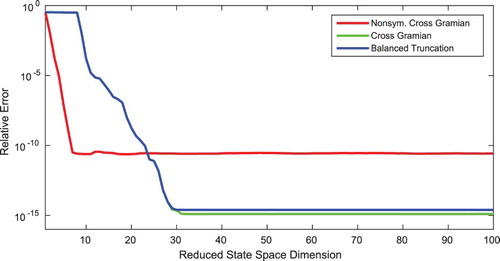
Figure 1 shows that the reduced-order models obtained by balanced truncation and the cross Gramian exhibits the same behaviour due to the state-space symmetric nature of the system. The newly proposed non-symmetric cross Gramian from Definition 3.1 does not achieve the same accuracy, but provides a lower output error for smaller reduced-order models. A lower accuracy is to be expected due to the use of a one-sided projection, while balanced truncation uses a two-sided Petrov–Galerkin projection, which in the state-space symmetric case is equal to the projection obtained from the (symmetric) classic cross Gramian. Notably, the output error of the reduced-order model from the non-symmetric cross Gramian drops already at a very low order to the steady error level while balanced truncation and the classic cross Gramian reach this error not until a reduced order of .

Figure 1. Relative output error of reduced-order models for reduced orders up to one hundred by balanced truncation, cross Gramian and non-symmetric cross Gramian for the state-space symmetric MIMO system.

Secondly, the non-symmetric cross Gramian is compared to balanced truncation and the approximate cross Gramian (5(5) ) of the symmetric system derived by embedding from Equation (5(5) ) for a non-square (and thus non-symmetric) system.

To prevent the computation of a symmetrizer matrix J, the symmetric system matrix from the first example is reused, yet now, a uniformly random generated input matrix for a single input and a uniformly random output matrix is selected, thus the system is non-square and non-symmetric, since M=1 and . Also for this example, zero initial state and impulse input are applied and the relative output error is evaluated for varying reduced-order state-space dimensions in Figure 2.

Figure 2. Relative output error of reduced-order models for reduced orders up to one hundred by balanced truncation, embedding cross Gramian and non-symmetric cross Gramian for a non-square SIMO system.

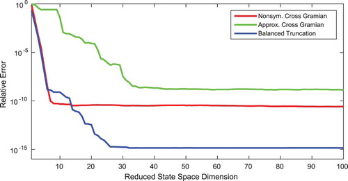
Using balanced truncation as reference, the cross Gramian of the embedded system performs worse as predicted in Sorensen and Antoulas (2001, 2002). Here, the output error of the balanced-truncation-based reduced-order model decays for an increasing reduced order largely with the same rate as the non-symmetric cross-Gramian-based reduced-order model.

Thirdly, a square but non-symmetric stable system with system matrix , uniformly random input matrix and uniformly random output matrix is chosen. For this system, balanced truncation, the cross Gramian and the non-symmetric cross Gramian are compared. Due to the non-symmetric nature of the system, the cross Gramian has no theoretical foundation, yet is applicable since the system is square. Heuristically, also in Baur and Benner (2008) workable results for non-symmetric systems have been obtained for the classic cross Gramian.

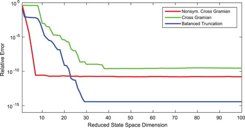
Figure 3 shows a similar results as for the non-square system: the reduced-order models by the cross Gramian and non-symmetric cross Gramian both exhibit a lesser accuracy, yet the non-symmetric cross Gramian's reduced-order models require the least states to reach this error level even compared to balanced truncation.

Figure 3. Relative output error of reduced-order models for reduced orders up to one hundred by balanced truncation, cross Gramian and non-symmetric cross Gramian for a non-symmetric, but square, MIMO system.

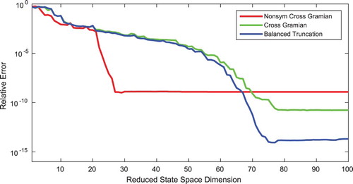
Next, the structural model for the Russian ISS service module 1r, which is part of the benchmark collection (Chahlaoui & VanDooren 2005), is tested. This model is a second-order square MIMO system of order N=270 and M=Q=3. As for the previous experiments, a zero initial state and an impulse input is utilized. For this benchmark, balanced truncation, direct truncation of the cross Gramian and direct truncation of the non-symmetric cross Gramian are applied. Due to the second-order nature of the system, a structure preserving variant of the truncation methods is chosen (Teng 2012).

Figure 4 shows a similar result as for the previous experiments. The error decay for increasing reduced order of the reduced-order models derived by the regular cross Gramian and balanced truncation is similar, but a lower error is reached by balanced truncation. The error of the reduced-order model resulting from the non-symmetric cross Gramian decays steeper but does not reach the same accuracy than the regular cross Gramian and balanced truncation.

Figure 4. Relative output error of reduced-order models for reduced orders up to one hundred by balanced truncation, cross Gramian and non-symmetric cross Gramian for the ISS-1r benchmark.

Lastly, a second benchmark from the collection (Chahlaoui & VanDooren 2005) is tested in an adapted form. The benchmark entitled ‘FOM’ (Chahlaoui & VanDooren 2005) describes a SISO system of order 1006. In Heyouni, Jbilou, Messaoudi, and Tabaa (2008), this benchmark is extended to a MIMO system, related to this adaption, in this setting a single-input-multiple-output (SIMO) variant of the benchmark is used. The system matrix is a block diagonal matrix consisting of four blocks, The input matrix (vector) from the original benchmark, is used. The output matrix is originally set to , in this setting the output matrix is generated by samples from a uniform random distribution with ranges, for each row of C, determined by :

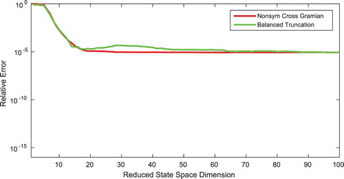
In Figure 5, the error for the non-square and thus non-symmetric adapted benchmark model are shown for balanced truncation and the non-symmetric cross Gramian. For this benchmark, the reduced-order models from balanced truncation and the non-symmetric cross Gramian perform similar in decay and lowest reached error. Notably, both methods coincide in their lowest attained error.

Figure 5. Relative output error of reduced-order models for reduced orders up to one hundred by balanced truncation and non-symmetric cross Gramian for the non-square variant of the FOM benchmark.

For all five experiments, the minimal state-space model reduction error of the presented non-symmetric cross Gramian is equal or worse than for balanced truncation, but the descent of the error is steeper or at least equally fast. Hence, if the lower accuracy is acceptable, often a smaller reduced-order model can be constructed with this (non-symmetric) variant of the cross Gramian method. This superior performance of the non-symmetric cross Gramian compared to balanced truncation and the regular cross Gramian (if applicable) for low-order reduced-order models is not yet supported by a theoretical result. Further investigation of the relation between a MIMO system and its associated ‘average’ SISO system with respect to linear superposition of linear system state and output could reveal an explanation for these surprising numerical results. Alternatively, the connection to the frequency-domain through the tangential cross Gramian may also uncover the reason for the model reduction performance of the non-symmetric cross Gramian.

In terms of computational complexity, the non-symmetric cross Gramian can be computed as the regular cross Gramian of the ‘average’ system, thus it has the same complexity as solving a Sylvester equation for a cross Gramian of a (linear) SISO system. From an empirical Gramian viewpoint, the non-symmetric empirical cross Gramian requires additional Q matrix additions to average the ‘observability’ snapshots compared to the regular empirical cross Gramian for a square (possibly nonlinear) system.

It should be noted that the non-symmetric cross Gramian is not suitable for frequency-space-based approximation. This is due to its construction by averaging the subsystem cross Gramians. For example, the (Hardy) -error between full and reduced-order model will decay very slowly or not at all, hence this method is currently targeted purely at state-space approximations.

7. Conclusion

In this work, a non-symmetric cross Gramian, based on concepts from decentralized control, is proposed, connected to the tangential interpolation method and demonstrated to provide viable results for linear non-symmetric and non-square systems, which are outside the scope of the regular cross Gramian.

Future work will evaluate the effectiveness of the non-symmetric cross Gramian for parametric and nonlinear systems. Furthermore, since the procedure for cross-Gramian-based Petrov–Galerkin projections suggested in Rahrovani, Vakilzadeh, and Abrahamsson (2014) does generally not yield stable reduced-order models in this setting, an investigation of two-sided and stability-preserving projections for the (non-symmetric) cross Gramian may yield errors comparable to balanced truncation.

Acknowledgments

The authors would like to thank the reviewers for pointing out the relation to the tangential interpolation method.

Disclosure statement

No potential conflict of interest was reported by the authors.

ORCiD

C. Himpe http://orcid.org/0000-0003-2194-6754

M. Ohlberger http://orcid.org/0000-0002-6260-3574

Additional information

Funding

This work was supported by the Deutsche Forschungsgemeinschaft, DFG EXC 1003 Cells in Motion – Cluster of Excellence, Münster, Germany as well as by the Open Access Publication Fund of the University of Münster and the Center for Developing Mathematics in Interaction, DEMAIN, Münster, Germany.

Notes

1 Equivalently, the symmetry of the impulse response, system gain or Markov parameter can be used.

2 Where the reduced-order components , , are derived by projections and .

3 For an overview on model reduction techniques see Antoulas (2005).

4 The balanced truncation is performed using the empirical controllability and observability Gramians.

References

- Alavian, A., & Rotkowitz, M. C. (2015). On a Hankel-based measure of decentralized controllability and observability. Fifth IFAC workshop on distributed estimation and control in networked systems. IFAC-Papers Online, 48(22), 227–232.
- Aldhaheri, R. W. (1991). Model order reduction via real Schur-form decomposition. International Journal of Control, 53(3), 709–716. doi: 10.1080/00207179108953642
- Antoulas, A. C. (2005). Approximation of large-scale dynamical systems. Advances in design and control (Vol. 6). Philadelphia, PA: SIAM.
- Antoulas, A. C., Beattie, C. A., & Gugercin, S. (2010). Interpolatory model reduction of large-scale dynamical systems. In Efficient modeling and control of large-scale systems (pp. 3–58). New York: Springer.
- Bartels, R. H., & Stewart, G. W. (1972). Solution of the matrix equation [F4]. Communications of the ACM, 15(9), 820–826. doi: 10.1145/361573.361582
- Baur, U., & Benner, P. (2008). Cross-Gramian based model reduction for data-sparse systems. Electronic Transactions on Numerical Analysis, 31, 256–270. Retrieved from eudml.org/doc/130548
- Baur, U., Benner, P., & Feng, L. (2014). Model order reduction for linear and nonlinear systems: A system-theoretic perspective. Archives of Computational Methods in Engineering, 21(4), 331–358. doi: 10.1007/s11831-014-9111-2
- Benner, P. (2004). Factorized solution of Sylvester equations with applications in control. Proceedings of the sixteenth international symposium on mathematical theory of network and systems (pp. 1–10). Retrieved from www.de.mpi-magdeburg.mpg.de/mpcsc/benner/pub/b_mtns04.pdf
- Chahlaoui, Y., & Van Dooren, P. (2005). Benchmark examples for model reduction of linear time-invariant dynamical systems, In P. Benner, V. Mehrmann, & D. C. Sorensen (Eds.), Dimension reduction of large-scale systems, Lecture Notes in Computational Science and Engineering (Vol. 45, pp. 379–392). Heidelberg: Springer.
- Datta, K. (1988). The matrix equation XA−BX=R and its applications. Linear Algebra and its Applications, 109, 91–105. doi: 10.1016/0024-3795(88)90200-5
- De Abreu-Garcia, J. A., & Fairman, F. (1986). A note on cross Grammians for orthogonally symmetric realizations. IEEE Transactions on Automatic Control, 31(9), 866–868. doi: 10.1109/TAC.1986.1104421
- Fernando, K. V., & Nicholson, H. (1983). On the structure of balanced and other principal representations of SISO systems. IEEE Transactions on Automatic Control, 28(2), 228–231. doi: 10.1109/TAC.1983.1103195
- Fernando, K. V., & Nicholson, H. (1985). On the cross-Gramian for symmetric MIMO systems. IEEE Transactions on Circuits and Systems, 32(5), 487–489. doi: 10.1109/TCS.1985.1085737
- Fortuna, L., Gallo, A., Guglielmino, C., & Nunnari, G. (1988). On the solution of a nonlinear matrix equation for MIMO symmetric realizations. Systems & Control Letters, 11(1), 79–82. doi: 10.1016/0167-6911(88)90115-6
- Gallivan, K., Vandendorpe, A., & Van Dooren, P. (2004). Model reduction of MIMO systems via tangential interpolation. SIAM Journal on Matrix Analysis and Applications, 26(2), 328–349. doi: 10.1137/S0895479803423925
- Gugercin, S., & Antoulas, A. C. (2000). A comparative study of 7 algorithms for model reduction. Proceedings of the 39th IEEE conference on decision and control (Vol. 3, pp. 2367–2372). Sydney, Australia.
- Heyouni, M., Jbilou, K., Messaoudi, A., & Tabaa, K. (2008). Model reduction in large scale MIMO dynamical systems via the block Lanczos method. Computational & Applied Mathematics, 27, 211–236. doi: 10.1590/S0101-82052008000200006
- Himpe, C. (2016). emgr – Empirical Gramian Framework (Version 3.9). http://gramian.de.
- Himpe, C., & Ohlberger, M. (2013). A unified software framework for empirical Gramians. Journal of Mathematics, 2013, 1–6. doi: 10.1155/2013/365909
- Himpe, C., & Ohlberger, M. (2014). Cross-Gramian-based combined state and parameter reduction for large-scale control systems. Mathematical Problems in Engineering, 2014, 1–13. doi: 10.1155/2014/843869
- Khaki-Sedigh, A., & Shahmansourian, A. (1996). Input–output pairing using balanced realisations. Electronics Letters, 32(21), 2027–2028. doi: 10.1049/el:19961346
- Lall, S., Marsden, J. E., & Glavaski, S. (1999). Empirical model reduction of controlled nonlinear systems. Proceedings of the IFAC world congress, F (pp. 473–478). Retrieved from authors.library.caltech.edu/20343/2/10.1.1.123.4669.pdf
- Laub, A. J., Silverman, L. M., & Verma, M. (1983). A note on cross-Grammians for symmetric realizations. Proceedings of the IEEE, 71(7), 904–905. doi: 10.1109/PROC.1983.12688
- Minh, H. B., & Batlle, C. (2013). optimal model reduction – Wilson's conditions for the cross-Gramian (Technical Report). Hanoi University of Science and Technology, Universitat Politécnica de Catalunya. Retrieved from www-ma4.upc.edu/carles/fitxers/h2_cross_gramian_v3.pdf
- Mironovskii, L. A., & Solv'eva, T. N. (2015). Analysis of multiplicity of Hankel singular values of control systems. Automation and Remote Control, 76(2), 205–218. doi: 10.1134/S0005117915020022
- Moaveni, B., & Khaki-Sedigh, A. (2006). Input–output pairing based on Cross-Gramian matrix. International joint conference SICE-ICAS (pp. 2378–2380). Busan, Korea.
- Moore, B. (1981). Principal component analysis in linear systems: Controllability, observability, and model reduction. IEEE Transactions on Automatic Control, 26(1), 17–32. doi: 10.1109/TAC.1981.1102568
- Pernebo, L., & Silverman, L. (1982). Model reduction via balanced state space representations. IEEE Transactions on Automatic Control, 27(2), 382–387. doi: 10.1109/TAC.1982.1102945
- J. R. Phillips, & Silveira, L. M. (2005). Poor man's TBR: A simple model reduction scheme. IEEE Transactions on Computer-Aided Design of Integrated Circuits and Systems, 1(240), 43–55. doi: 10.1109/TCAD.2004.839472
- Rahrovani, S., Vakilzadeh, M. K., & Abrahamsson, T. (2014). On Gramian-based techniques for minimal realization of large-scale mechanical systems. In R. Allemang, J. De Clerck, C. Niezrecki, & A. Wicks (Eds.), Topics in modal analysis. (Vol. 7, pp. 797–805). New York: Springer.
- Shaker, H. R., & Tahavori, M. (2015). Control configuration selection for bilinear systems via generalised Hankel interaction index array. International Journal of Control, 88(1), 30–37. doi: 10.1080/00207179.2014.938250
- Shampine, L. F. (1965). The condition of certain matrices. Journal of Research of the National Bureau of Standards, 69B(4), 333–334. Retrieved from nvlpubs.nist.gov/nistpubs/jres/69B/jresv69Bn4p333_A1b.pdf doi: 10.6028/jres.069B.034
- Sorensen, D. C., & Antoulas, A. C. (2001). Projection methods for balanced model reduction (Technical Report) (pp. 1–18). Retrieved from http://www.caam.rice.edu/caam/trs/2001/TR01-03.pdf
- Sorensen, D. C., & Antoulas, A. C. (2002). The Sylvester equation and approximate balanced reduction. Linear Algebra and its Applications, 351, 671–700. doi: 10.1016/S0024-3795(02)00283-5
- Sorensen, D. C., & Antoulas, A. C. (2005). On model reduction of structured systems. In P. Benner, V. Mehrmann, & D. C. Sorensen (Eds.), Dimension reduction of large-scale systems, Lecture Notes in Computational Science and Engineering (Vol. 45, pp. 117–130). Heidelberg: Springer.
- Streif, S., Findeisen, R., & Bullinger, E. (2006). Relating cross Gramians and sensitivity analysis in systems biology. Proceedings of the 17th international symposium on mathematical theory of networks and systems, 10.4 (pp. 437–442). Retrieved from eprints.nuim.ie/1768/1/HamiltonGramian.pdf
- Teng, C. (2012). Second-order model reduction based on Gramians. Journal of Control Science and Engineering, 2012, 1–9. doi: 10.1155/2012/302498
- Willems, J. C. (1976). Realization of systems with internal passivity and symmetry constraints. Journal of the Franklin Institute, 301(6), 605–621. doi: 10.1016/0016-0032(76)90081-8
- Zhou, K., Salomon, G., & Wu, E. (1999). Balanced realization and model reduction for unstable systems. International Journal for Robust Nonlinear Control, 3(9), 183–198. doi: 10.1002/(SICI)1099-1239(199903)9:3<183::AID-RNC399>3.3.CO;2-5