Heuristic grey-box modelling for photovoltaic power systems

ABSTRACT

Amongst non-conventional generators, photovoltaics (PVs) are becoming more popular owing to their relatively low costs and convenience. However, the intermittency of the PV generator outputs require accurate forecasting, planning, and optimal management. Existing forecasting methods, which are based on either clear-box or black-box modelling, have room for improvement, especially in the accuracy of capturing the underlying PV characteristics and forecasting of PV yields. This paper explores the use of a priori knowledge of PV systems to heuristically improve their clear-box and black-box models. The paper then further explores the use of heuristic grey-box modelling to identify uncertain parameters of physical principle. Incorporating black boxes to account for such un-modelled uncertainties inherent in a clear box provides the resultant grey box with improved forecasting performance and offers a new approach to practical system modelling. The experimental results on an installed PV system have confirmed the usefulness of this approach.

KEYWORDS:

• Photovoltaic
• renewable energy
• neural networks
• particle swarm optimization
• heuristics
• grey-box modelling

1. Introduction

Photovoltaic (PV) is now positioned amongst the top three new power generation sources installed in Europe and this trend is expected to stay (Global Market Outlook for photovoltaics 2013–2017, 2013, May). Power from PV sources provides a number of benefits over other renewable energy sources (RESs). It can be supplied locally to loads, reducing the cost of transmission lines and their associated power losses. Furthermore, advances in technology and large-scale manufacturing have led to the decline in PV costs at a steady rate (Swanson, 2009). Despite a substantial capital setup cost, PV operation and maintenance cost is almost zero (Renewable Energy Technologies: Cost Analysis Series, Photovoltaics, 2012).

Nonetheless, like other RES, PV sources pose a number of integration challenges to the grid. A major criticism of PV sources is the variability in irradiance due to cloud transients and diurnal effects, which has negative impacts on the grid’s voltage profile (Stetz, Marten, & Braun, 2013; Woyte, Thong, Belmans, & Nijs, 2006). In particular, intermittency of the PV sources is a major factor affecting the load following capabilities of the grid (Ma et al., 2012). While it is recognized that advance knowledge of the expected yield from PV sources will help tackle these challenges, to allow for proper planning of available generation sources and provide insights into the impact of PVs on the power network, accurate forecasting of PV yield is not a trivial task. This can be largely attributed to the non-continuous and nonlinear nature of PV sources, which are due to the interplay of factors such as the variability in sunrise and the amount of sunshine, sudden changes in atmospheric conditions, cloud movements and dust (Cibulka, Brown, Miller, & Meier, 2012). The PV power data can thus be viewed as consisting of two parts: the deterministic and the stochastic. The former represents the mathematical equations of irradiance that depend on location, sun’s position, and equations of PV cells, whilst the latter represents the sudden atmospheric changes such as dust, clouds, and wind blow.

Various mathematical models, such as first principle-based clear-box models, have been developed to forecast the PV yield. With underlying PV physics, these models provide a structured and meaningful forecast of power outputs and typically require fewer parameters to estimate than other models (Forsell & Lindskog, 1997), such as a black-box-based generic approximation models. Compared with black-box models, however, clear boxes are less accurate, especially for large systems (Tao, Shanxu, & Changsong, 2010). This is because in reality, most systems are complex and nonlinear and often contain dynamics that are hard to capture mathematically.

Black-box models are data driven and can be based on statistics in approximating nonlinear systems. They have found broad applications in engineering practice, including handling nonlinear time series, as they are relatively simpler to use. For example, dynamic neural networks (DNN) such as the ‘focused time-delay neural networks’ (FTDNN) and the ‘distributed time-delay neural networks’ have been applied to the PV forecasting problem (Al-Messabi, Li, El-Amin, & Goh, 2012). Black-box models however require good data – with both quality and quantity – for an accurate forecast, and its lack of underlying physics makes it hard to understand the results and their causes. Such models are also difficult to design structurally due to the large number of parameters required because of missing physics.

This paper focuses on the development of a grey-box model, which takes advantages of both the black-box and the clear-box models (Tan & Li, 2002), for the identification of improved PV models. The work reported starts with a clear-box model followed by a simple black-box model, and then grey-box models. Section 2 provides an overview of related work on clear-box models for solar PV modelling. Section 3 develops a clear-box PV model using manufacturer data. Section 4 develops a data-driven FTDNN black-box model. In Section 5, uncertain parameters in the clear-box model are identified and optimized using heuristic Direct Pattern search (PS) and particle swarm optimization (PSO) algorithms, resulting in an evolutionary clear-box model. In Section 6, the evolutionary model is extended to grey-box models to account for unknown effects at forecast. Results and observations are discussed in Section 7 and conclusions are drawn in Section 8.

2. Solar PV generator models

2.1. PV data-driven moldelling overview

There exist various forecasting models for PV systems (Al-Messabi et al., 2012; Duffie & Beckman, 2006; Fernandez-Jimenez et al., 2012; Forsell & Lindskog, 1997; Gow & Manning, 1999; Ma et al., 2012; Mellit & Pavan, 2010; Stetz et al., 2013; Swanson, 2009; Temps & Coulson, 1977; del Valle, Venayagamoorthy, Mohagheghi, Hernandez, & Harley, 2008; Woyte et al., 2006). The simplest ones are ‘naïve’ or persistence models, where the next power value is assumed to be the same as at the previous step. Such models are usually taken as reference models in forecasting studies (Bacher, Madsen, & Nielsen, 2009).

Another approach to forecasting PV power is to model solar data using statistical methods. Regression models are used to express power values as a regression of previous power values, irradiance, and temperature (Kroposki, Emery, Myers, & Mrig, 1994). Statistical approaches adopt classical time-series forecasting methods that assume the data stationary. Auto-regressive (AR), AR with exogenous input, and AR with integrated moving average (Bacher et al., 2009) are some of the well-known statistical models used in solar PV forecasting. As the parameters in these models usually do not represent a physical phenomenon or quantity, such models are often referred to as ‘black-box’ models or a type of functional approximators. The artificial neural network (NN) is another example of these models and is gaining popularity in PV forecasting owing to their modularity in handling nonlinear models. There are various structures of an NN, but they can be categorized into two according to their temporal characteristics: the static NN (Mellit & Pavan, 2010) and the dynamic NN (Fernandez-Jimenez et al., 2012). However, data-fit models can suffer from a generalization deficiency. Further, there is no systematic way in arriving at the most appropriate structure of the model due to omitting the underlying physics.

An alternative to this is the ‘clear-box’ model based on physical principles. The benefits of these models were outlined in the introduction and their equations are detailed in the preceding section.

2.2. PV module physical equations

There are various physical-principle-based models developed for PV modules, for example, a double diode model (Gow & Manning, 1999), a simplified single diode model (SSDM), and further SSDMs in a descending order of complexity. Higher complexity can provide better accuracy on the expense of increased computational burden, which is not suitable for real-time or online applications.

The best model that gives a good compromise between simplicity and accuracy is the SSDM shown in Figure 1 (Villalva, Gazoli, & Filho, 2009).

Figure 1. PV cell/array single diode simplified model.

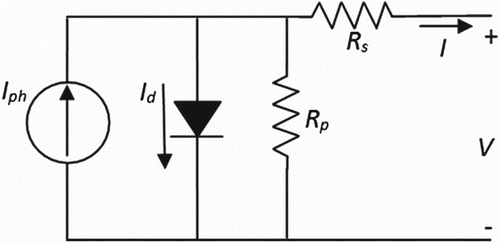
The following equations describe the relation between the current and voltage output of the PV cell/array: (1) (2) where I is the output current of the cell in amperes, V is the solar cell voltage in volts, I_ph is the photocurrent in amperes, I_d is the Shockley diode equation, I_o is the reverse saturation or leakage current of the diode, V_t = kT/q is the thermal voltage of the array, q is the electron charge (1.60217646 × 10⁻¹⁹ C), k is the Boltzman constant (1.3806503 × 10^–23 J/K), T is the temperature of the cell in kelvin, and a is the ideality factor constant. More details of these equations can be found in Villalva et al. (2009). To calculate power yield, values for I and V are usually computed using numerical methods (Gow & Manning, 1999; Villalva et al., 2009). The mathematical approach is usually tedious especially when applied to large or widely spread PV systems (Tao et al., 2010).

2.3. Simplified PV equations

The aforementioned equations of PV modules require numerical solutions and thus are sometimes replaced with simplified equations that relate the power output to the efficiency of the system and variation in radiation and temperature (Omran, Kazerani, & Salama, 2010; Osterwald, 1986). These equations are a translation of performance measurement from standard test conditions (STC; Air Mass 1.5 spectrum with global irradiance G = 1000 W/m² and module temperature = 25°C). One famous simple method is that of Osterwald (1986), which can be described as follows: (3) where P_m is the cell/module maximum power (W), P_mo is the cell/module maximum power in STC (W), is the cell maximum power coefficient (°C⁻¹), which ranges from −0.005 to −0.003°C⁻¹ in crystalline silicon and can be assumed to be −0.0035°C⁻¹ with good accuracy.

Another version of Equation (3) is given below (Omran et al., 2010): (4) where G_t is the global irradiance on the titled surface in W/m², K_T is thermal derating coefficient of the PV module in %/°C, A_a area of the PV array in m², η_m is the module efficiency, η_dust is 1-the fractional power loss due to dust on the PV array, η_mis is 1 – the fractional power loss due module mismatch, η_DCloss is 1 – the fractional power loss in the DC side, η_MPPT is 1 – fractional power loss due to the maximum power point tracking (MPPT) algorithm, T_C is the cell temperature in °C, T_ao is the ambient temperature at STC conditions in °C. The ac power of the PV system is then estimated by using manufacturer’s efficiency curve of three phase inverter.

The simplified PV equation adopted for this work is given below (Rahman & Yamashiro, 2007): (5)

In this equation, miscellaneous losses including dust were lumped together in η_loss; PV cell efficiency η_PV and MPPT or inverter efficiency η_inv are kept separate. T_m is the module temperature.

The aforementioned Equations (3)–(5) require detailed modelling of the global irradiance falling on a tilted surface G_t as outlined in the next section.

2.4. Irradiance falling on a tilted surface: Hottel’s equations

There exist various models for calculating irradiance on a tilted panel. However, some of these models rely on other meteorological data such as total irradiance on horizontal surface, diffuse irradiance on horizontal surface, and beam normal irradiance. Models of this type include those of Perez, Scott, and Stewart (1983), Perez, Seals, Ineichen, Stewart, and Menicucci (1987) and Klucher (1979). Others are not accurate in cloudy conditions, Temps and Coulson (1977), or in clear skies, Liu and Jordan (1963). Simple models that require no additional solar measurements were proposed by Hottel (Chupong & Plangklang, 2011; Duffie & Beckman, 2006; Hottel, 1976; Tao et al., 2010) and are adopted in this work. Description of this model is outlined as follows.

To explain irradiance equations, it is important first to present equations of solar angles as they are a pre-requisite to calculate solar equations. The derivation of irradiance on tilted surfaces requires the calculation of different solar angles. These equations are mainly based on Duffie & Beckman (2006); Iqbal (1983). Solar angles that define the position of the sun with respect to a PV plane are illustrated in Figure 2.

Figure 2. Solar angles of a PV plane.

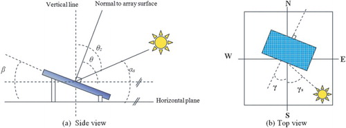
In Figure 2, β = tilt angle of array; Α_s = solar elevation (altitude): the angle between the horizontal and line to the sun; θ = angle of incidence: the angle between normal to array surface and direct irradiance on a tilted surface (or line to the sun); θ_z = zenith angle: the angle between vertical line to earth and line to the sun; γ_s = solar azimuth angle: the angular displacement from south of the projection of beam radiation on the horizontal plane. Displacements east of south are negative and west of south are positive; γ = surface azimuth angle: the deviation of the projection on a horizontal plane of the normal to the surface from the local meridian, with zero due to south, east negative, and west positive; −180°≤ γ ≤ 180°.

The zenith angle θ_z can be written as follows: (6) where δ is the declination angle given by (7) and ϕ = the latitude in degrees is the angular location north or south of the equator, north positive; −90° ≤ ϕ ≤ 90°; ω = the hour angle which is the angular displacement of the sun east or west of the local meridian due to rotation of the earth on its axis at 15° per hour; morning negative, afternoon positive. The hour angle can be calculated by first calculating the solar time given by (8) where L_st is the standard meridian for the local time zone, L_loc is the longitude of the location in question, and longitudes are in degrees west. The parameter E is the equation of time in minutes and is given by (9) where B is calculated as follows: (10) The hour angle ω can then be written as (11) Furthermore, the incidence angle θ can be calculated using the following formula: (12)

The solar irradiance falling on a tilted surface, G_t (W/m²) is composed of three parts: the direct irradiance G_tb (W/m²), the diffuse irradiance G_td (W/m²), and reflected irradiance G_tr (W/m²), that is, (13)

The three components of irradiance can be calculated as follows: (14) (15) (16) where G_on is the extraterrestrial radiation (W/m²), τ_b is the beam atmospheric transmittance, τ_d is the diffuse atmospheric transmittance, and τ_r is the reflected atmospheric transmittance. G_on can be calculated as follows: (17) where G_sc is 1367 ± 5 W/m² and d is the day of the year.

The atmospheric transmittances atmospheric transmittances, τ_b, τ_d, and τ_r can be calculated as follows: (18) where a₀, a₁, and k are constants that can be calculated as follows: (19) (20) (21) where A is the altitude of the location in km, r₀, r₁, and r_k are correction factors for different types of climates and are given in Table 1.

3. Clear-box approach to PV modelling

The test-bed system, located in the sunny city of Masdar, close to Abu Dhabi airport, is a 220,000 m², 10 MW PV plant (10MW Solar Power Plant, Enviromena Power Systems Report, 2014; Masdar City Solar PV Plant, n.d.). The plant consists of around 87,777 panels: 17,777 being polycrystalline and 70,000 being thin-film from Suntech and First Solar, respectively. The parameters for the model were taken from data sheets of panels (SunTech: SunTech panel data sheet: STP270S – 20/Wd+, STP265S – 20/Wd+, 2014) (FS Series 2 PV Module PD-5-401-02 NA May, 2011) and from engineers in Masdar. These parameters, which are best engineering values taken from data sheet and engineers’ measurements on the PV system, are given in Table 2. The model with these values yields a clear-box model.

Table 1. Coefficient values dependent on climate.

Climate type	r0	r1	rk
Tropical	0.95	0.98	1.02
Midlatitude summer	0.97	0.99	1.02
Subarctic summer	0.99	0.99	1.01
Midlatitude winter	1.03	1.01	1.00

Table 2. Parameters of the clear-box PV model.

Parameters	Values
Longitude	54.45°
Latitude	24.43°
Altitude	1 m
Area of SunTech panels, ASun	30,911 m^2
Area of First Solar panels, AFirst	72,500 m^2
Miscellaneous losses (Suntech group), ηloss_Sun	5% (i.e. ηloss_Sun = 95%)
Miscellaneous losses (Firstsolar group), ηloss_First	6% (i.e. ηloss_First = 94%)
Efficiency of PV panel (Suntech), ηPV_Sun	11%
Efficiency of PV panel (Firstsolar), ηPV_First	10%
Efficiency of inverter (Suntech panels), ηinv_Sun	95%
Efficiency of inverter (Firstsolar), ηinv_First	94%
Temperature coefficient (%/C°), γ	0.5%
r0	0.27
r1	0.29
r2	0.32
Albedo, ρ	0.35

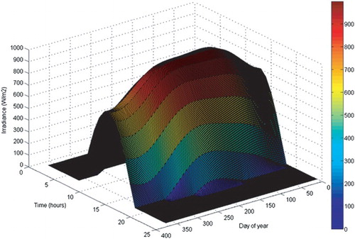
The clear irradiance model based on Hottel’s Equations (6)–(21) was simulated; one year irradiance values are plotted in Figure 3. These values represent clear-sky values expected to fall on Masdar PV panels.

Figure 3. Clear-day irradiance model for one year.

Furthermore, the expected yield from the PV plant was simulated using Equation (5), where values of parameters given in Table 2 were used. Power yield for five days in July and January are given in Figures 4 and 5, respectively.

Figure 4. Clear box: PV power and error plot for 20–24 July 2010.

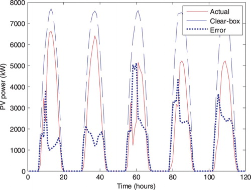
Figure 5. Clear box: PV power and error plot for 20–24 January 2011.

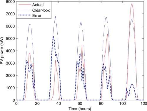
The absolute error residuals between modelled and actual power were calculated and shown in Figures 4 and 5. To measure the accuracy of the model, the Root Mean Square Error (RMSE) between actual and identified model in terms of PV power output was calculated. The RMSE is calculated as follows: (22) where is the ith actual output power, is the ith predicted power by model, and n is number of data points. The RMSE for the clear-box model is given in Table 6. The error plot and RMSE indicate large errors when standard values are used in the clear-box models. It also indicates that the error changes with yield of the PV system.

4. Enhancement of clear-box PV model

The clear-box model assumes that different parameters, with values outlined in data sheet, are constant all time. However, in reality, values change with variations in atmospheric conditions and degradation of materials. For the PV system studied in this work, uncertainties in the operating values of parameters such as PV efficiencies, albedo of ground, temperature coefficient and miscellaneous losses may have contributed to the under par forecasting performance. It is possible to further enhance the accuracy of the clear-box model by identifying optimal values for these parameters. Heuristic algorithms are ideal candidates for handling uncertainties since they are based on ‘intuitive’ learning and do not strictly require formulas to work. Here, two such heuristic algorithms, namely a PS and a swarm intelligence-based search, are applied to tune the clear-box model.

4.1. PS approach

A simple derivative-free direct PS method, suitable for a constrained search problem, is first used to find the best set of values for the parameters outlined in Table 3. The concept of the algorithm is to search a mesh of points around the current initial point. The pattern is a scalar multiple of a set of vectors that are added to the current point. If a point in the mesh provides an improved fitness value, it becomes the current point for the next iteration of the search.

Table 3. Range of uncertain parameters for evolutionary clear-box PV model.

Parameters	Values
ηloss_Sun	92–96%
ηloss_First	92–96%
ηPV_Sun	10–12%
ηPV_First	10–12%
ηinv_Sun	92–99%
ηinv_First	92–99%
γ	0.2–0.6%
r0	0.2–1.0
r1	0.2–1.0
r2	0.2–1.0
Ρ	0.3–0.5

The search seized as mesh size reached the minimum tolerance size (1 × 10⁻⁶). The initialization of the search required several repetitions as PS is sensitive to initial values.

The data obtained from the system was used in two phases: first to tune the model and second to validate its performance. The model is trained using the hourly PV power and module temperature) from days 5–20 in July 2010 (summer) and days 5–20 in January 2011 (winter). The fitness function of the identification is chosen as the average error of July and January as shown below: (23)

Once the model is identified, five consecutive days in both July 2010 and January 2011 are used to validate its performance. Forecasting error is measured using the average RMSE (RMSE_test).

The modelled output power and error plots are shown in Figures 6 and 7. The RMSE value is given in Table 6. The results obtained show an improvement (585.2 kW reduced error corresponding to a 36% improvement over clear-box model) in the forecasted output. This indicates that further enhancement of the clear-box model is possible when parameters are tuned to reduce uncertainties in the operating values. The list of identified parameters is given in Table 4.

Figure 6. PV power yield forecasts: actual vs. models (clear box, evolutionary clear box, grey box 1): 20–21 July 2010.

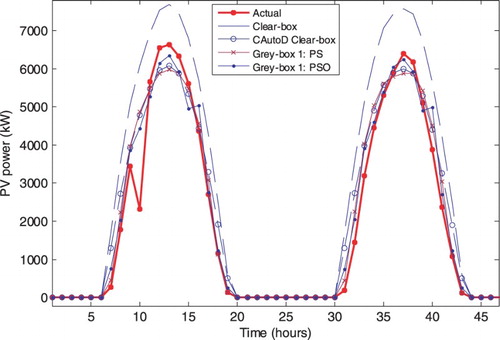
Figure 7. Absolute error of forecast for models in Figure 10: 20–21 July 2010.

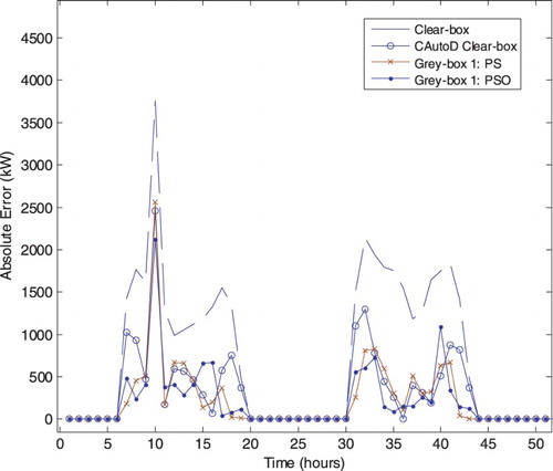
Table 4. Evolutionary clear-box PV model parameters identified by heuristic algorithms (PS and PSO): both reached same optimum parameters.

Parameters	Values
ηloss_Sun	92%
ηloss_First	92%
ηPV_Sun	10%
ηPV_First	10%
ηinv_Sun	92%
ηinv_First	92%
γ	0.46%
r0	0.2
r1	0.2
r2	1.0
ρ	0.3

4.2. PSO approach

PSO is inspired by the social behaviour of bird flocking or fish schooling (Eberhat & Shi, 2001). PSO has also been used here to optimize the parameters in the evolutionary clear-box model. For consistency, the same objective function of (23) was used in the optimization. The optimization including flying particles, potential solutions, in the dimension of solution space at different velocities. The particles’ positions and velocities are updated in each iteration until optimum solution is reached; details of the algorithm can be found in Kennedy, Eberhart, & Shi (2001).

The number of particles is set to n = 50 and the maximum number of search iterations at 500. The RMSE resulting from the PSO is given in Table 6. It is clear from the results obtained that with PSO enhancement; the clear-box model is able to achieve better forecasting accuracies. Nonetheless, no marked improvement was observed when compared to the PS enhanced clear-box model.

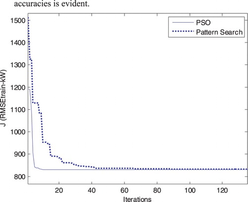
The convergence of both algorithms is shown in Figure 8. It is observed that whilst PSO took a shorter time to find the global minimum, more evaluations were required. This is mainly due to the higher numbers of initial particles and objective evaluations required in each iteration of the search process. On the other hand, PS is sensitive to initial conditions. For both methods, improvement in forecasting accuracies is evident.

Figure 8. Convergence of evolutionary clear-box identification.

5. Global black-box approach

Another simple approach to forecast PV power is to use time-series or data-driven models. Owing to the capability to handle nonlinearity and time-series data and absence of requirement for transformation to stationary data (Mellit & Pavan, 2010), DNN have been studied for PV forecasting; specifically FTDNN was explored (Al-Messabi et al., 2012). FTDNN was trained on PV power yield for days 5–20 in July 2010 (summer) and 5 days 5–20 in January 2011 (winter). The PV power of Masdar is of an hourly interval resolution. A similar approach to (Al-Messabi et al., 2012) was used in building a global PV FTDNN model. Delayed inputs of D = [1:10] are fed to the network, that is,

Eight neurons were chosen for the hidden layer. The network was tested for one to several steps ahead for the entire system. Five consecutive days in both July 2010 and January 2011 were used to test the models and to compute the average forecasting RMSE (RMSE_test). Average RMSE values for different step ahead forecasts are given in Figure 11. Sample plots of the forecasts are given in Figures 9 and 10.

Figure 9. FTDNN forecasts: 20–21 July 2010.

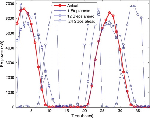
Figure 10. FTDNN forecasts: 22–23 January 2011.

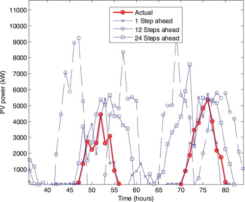
Figure 11. FTDNN forecast: average RMSE for several steps ahead.

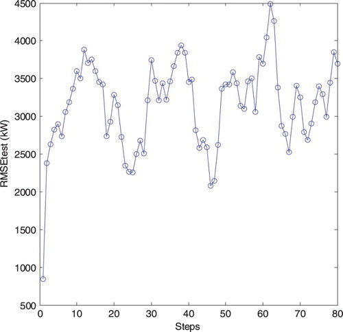
It is noted that the black-box FTDNN model is suitable for few steps (i.e. few hours) ahead where RMSE is comparable with clear-box values. However, for longer steps ahead, the error increases, although it shows a declining trend for days (24 and 48 hours) ahead forecast.

6. Heuritic grey-box PV modelling

Enhancement of the clear-box model is achievable by introducing local black-boxes to account for unknown effects. These represent nonlinearities not captured by the clear-box model. These will be accounted for by incorporating black-box parts to model operating-point sensitive coefficients. For example, in PVs, the parameters of efficiency of inverter are known to be adaptive and are function of their loading (Pregelj, 2003).

The black-box models incorporated can take any form of generic function approximators: power series polynomials, NNs, fuzzy logic, etc. In this work, we use polynomials and rational functions or the Pade approximators. The following two grey-box models are thus developed to accommodate changes in the clear-box efficiencies with loading:

Table

	Grey box 1
	Grey box 2

where P_o is the fractional loading calculated by dividing the P_DC output of PV by nominal DC rating of the inverter.

The first model, grey box 1, is based on Padé approximation while the second, grey box 2, needs higher order polynomials because of no denominator and hence no recursion in the approximation. Both will be artificially evolved for optimal PV models. The coefficients of these models will be identified again by PS and PSO such that objective function (23) is minimized with the same set of training and test data.

The heuristically evolved parameters of the models are given in Table 5. The accuracy of all the models is compared in Table 6.

Table 5. Grey-box PV models parameters identified by heuristic algorithms (PS and PSO).

	Grey box 1		Grey box 2
Parameters	PS	PSO	PS	PSO
ηloss_Sun	94.53%	92%	95.62%	96%
ηloss_First	92.39%	92%	92.68%	96%
ηPV_Sun	10.56%	10%	11.71%	10%
ηPV_First	11.09%	10%	10.45%	10%
γ	0.58%	0.60%	0.60%	0.23%
r0	0.8752	0.20	0.2532	1.0
r1	0.9246	0.20	0.2237	0.2
r2	0.20	0.20	0.9864	1
ρ	0.4827	0.30	0.3079	0.30
a1	8.3680	−1.8519	−2.1865	−7.1138
a2	−6.1473	0.8753	8.9707	0.5454
a3	−7.5293	2.4521	8.9761	6.3646
a4	4.2134	−4.4688	8.9602	−1.4631
a5	0.5883	1.9566	2.4498	−5.2401
a6	2.0300	7.8651	8.6680	0.0535
a7	−4.9851	1.6034	−8.4668	2.5518
a8	−1.4083	9	−4.6007	3.7275
a9	7.4832	5.7039	−1.9806	−8.2013
a10	7.1191	5.9855	5.0446	3.3683
a11	8.2709	9
a12	2.8033	−1.3610

Table 6. Average RMSE values for training and testing of models (5 days ahead in Winter (January) and Summer (July)).

Model	Identification method	RMSEtrain (kW)	RMSEtest (kW)
Clear box	Engineering values	–	1636.0
Evolutionary clear box	PS	830.5799	1050.8
	PSO	830.5781	1050.8
Grey box 1	PS	779.3292	1005.1
	PSO	767.4825	1000.6
Grey box 2	PS	1563.7	1771.6
	PSO	775.1598	992.527

Bold number are the minimum and maximum values (RMSE) in each column (Training and Testing columns respectively).

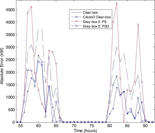
For grey box 1, the search algorithms produced closer results, and PSO slightly outperformed PS. For the higher order grey box 2, PS failed to find the optimum solution while PSO succeed. The progresses of the search for grey boxes 1 and 2 are shown in Figures 14 and 16, respectively. The power yields and absolute errors of the grey-box models are shown in Figures 12^{Figure 13Figure 14}–15 and 17^{Figure 18}–19. It can be seen that the grey boxes provide improved forecasts especially in transient period as power starts to rise or fall.

Figure 12. PV power yield forecasts: actual and forecast models (clear box, evolutionary clear box, grey box 1): 22–23 January 2011 (cloudy days).

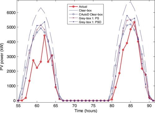
Figure 13. Absolute error of forecast for models in Figure 12: 22–23 January 2011.

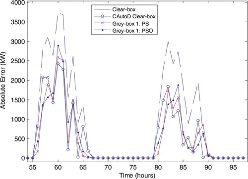
Figure 14. Convergence of grey box 1 identification.

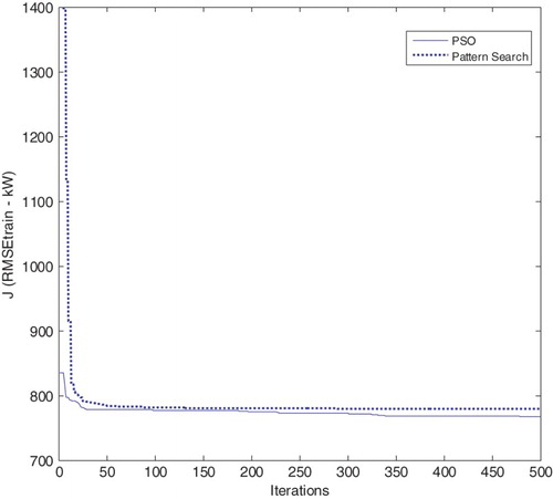
Figure 15. PV power yield forecasts: actual vs. models (clear box, evolutionary clear box, grey box 2): 20–21 July 2010.

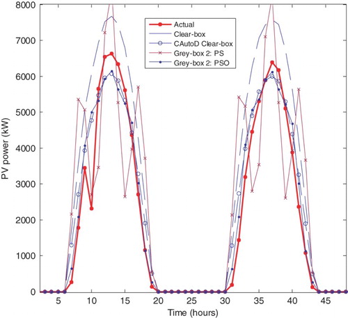
Figure 16. Convergence of grey box 2 identification.

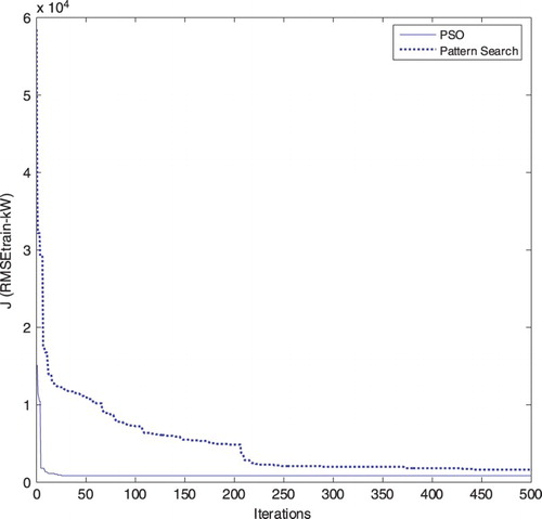
Figure 17. PV power yield forecasts: actual vs. models (clear box, evolutionary clear box, grey box 2): 22–23 January 2011.

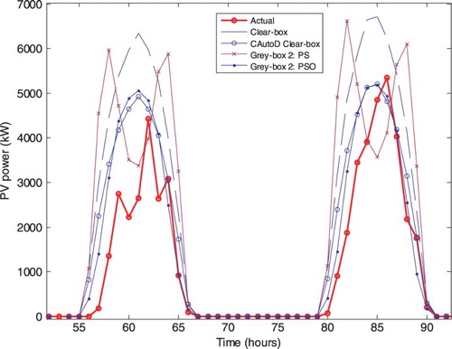
Figure 18. Absolute error of forecast for models in Figure 15: 20–21 July 2010.

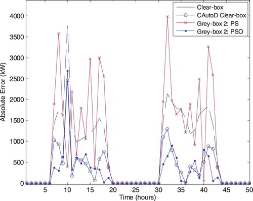
Figure 19. Absolute error of forecast for models in Figure 17: 22–23 January 2011.

7. Discussion of results

1. In general, tuning the parameters of a clear-box model improves forecasting results, as parameters from manufacturers require further calibration according to the specific atmospheric and location conditions of a given PV application.

2. Evolutionary clear-box models provide forecasts more accurately, especially on long horizons, than black-box FTDNN models.

3. Black-box models without exogenous inputs are found suitable only for very short horizon forecasting.

4. On the whole, grey-box models enhance the modelling accuracy compared with pure clear boxes and heuristically optimized Evolutionary clear-box models, as evident from both the training and the testing models. This is vivid in transient period of the power yield and in clear-sky days. It is also clear when comparing the RMSE values.

5. PS and PSO provided heuristic identification approaches to grey-box modelling. However, PS is sensitive to initial values and fails as models are of a high order. On the other hand, PSO goes through larger number of function evaluations depending on number of particles sent for the search journey.

6. Increasing or decreasing the order of grey boxes 1 and 2 is found to deteriorate the modelling or generalization accuracy and hence the given values are optimal numbers of the associated black boxes.

7. Generally the models coincides more with actual yield in clear days (such as in July) as they are based on clear-sky Hottel equations.

8. General observation: the simplified model, Equation (5), is found more sensitive to module temperature in July than in January, that is, excluding the temperature coefficient part (in brackets) has had a higher impact (worsen accuracy) in July than in January. This is expected as higher temperatures in July will impact the performance of the PV panels.

Areas of improvement include exploring different structures for grey-box models. Further, clear-box model can be explored to incorporate parameters replaced by black boxes to account for uncertainties.

8. Conclusion

The enhancement of clear-box modelling and forecasting of PV power through the introduction of black-box models has been studied and developed in this paper. It has been found that practical values of parameters can be tuned to improve the accuracy of the models. Further enhancement can be achieved through the introduction of grey-box models to account for uncertainties in the PV models. Derivative-free heuristics can be utilized in the identification processes, which has found particularly beneficial with grey-box model identification. The work presented is a novel step towards improved PV forecasting and a better integration of this RES in the power network.

Disclosure statement

No potential conflict of interest was reported by the authors.

References

- 10MW solar power plant, enviromena power systems report. (2014). Retrieved from http://enviromena.com/2015/wp-content/uploads/2014/01/10MW-Masdar_PD_2013-WEB.pdf
- Al-Messabi, N., Li, Y., El-Amin, I., & Goh, C. (2012, June 10–15). Forecasting of photovoltaic power yield using dynamic neural networks. In The 2012 international joint conference on neural networks (IJCNN) (pp. 1–5).
- Bacher, P., Madsen, H., & Nielsen, H. A. (2009). Online short-term solar power forecasting. Solar Energy, 83, 1772–1783. doi: 10.1016/j.solener.2009.05.016
- Chupong, C., & Plangklang, B. (2011). Forecasting power output of PV grid connected system in Thailand without using solar radiation measurement. Energy Procedia, 9, 230–237. doi: 10.1016/j.egypro.2011.09.024
- Cibulka, L., Brown, M., Miller, L., & Meier, A. V. (2012). User requirements and research needs for renewable generation forecasting tools that will meet the need of the CAISO and utilities for 2020. California: CIEE.
- Duffie, J., & Beckman, W. (2006). Solar engineering of thermal process (3rd ed.). New Jersey: John Wiley and Sons.
- Eberhat, R., & Shi, Y. (2001). Particle swarm optimization: Developments, applications, and resources. Proceedings of the 2001 Congress on Evolutionary Computation, 1, 81–86. doi: 10.1109/CEC.2001.934374
- European Photovoltaic Industry Association. (2013, May). Global market outlook for photovoltaics 2013–2017. Author.
- Fernandez-Jimenez, L. A., Munoz-Jimenez, A., Flaces, A., Mendoza-Villena, M., Garcia-Garrido, E., Lara-Santillan, P., … Zorzano-Santamaria, J. (2012). Short-term power forecasting system for photovoltaic plants. Renewable Energy, 44, 311–317. doi: 10.1016/j.renene.2012.01.108
- Forsell, U., & Lindskog, P. (1997). Combining semi-physical and neural network modelling: An example of its usefulness. Proceedings of the 11th IFAC Symposium on System Identification, 4, 795–798.
- Gow, J. A., & Manning, C. D. (1999, March). Development of a photovoltaic array model for use in power-electronics simulation studies. IEE Proceedings on Electric Power Applications, 146(2), 193–200. doi: 10.1049/ip-epa:19990116
- Hottel, H. C. (1976). A simple model for estimating the transmittance of direct solar radiation through clear atmospheres. Solar Energy, 18(2), 129–134. doi: 10.1016/0038-092X(76)90045-1
- Iqbal, M. (1983). An introduction to solar radiation. Toronto: Academic Press.
- Kennedy, J., Eberhart, R., & Shi, Y. (2001). Swarm intelligence. San Francisco: Morgan Kaufmann.
- Klucher, T. M. (1979). Evaluation of models to predict insolation on tilted surfaces. Solar Energy, 23, 111–114. doi: 10.1016/0038-092X(79)90110-5
- Kroposki, B., Emery, K., Myers, D., & Mrig, L. (1994). A comparison of photovoltaic module performance evaluation methodologies for energy ratings. Conference Record of The Twenty Fourth IEEE Photovoltaic Specialists Conference, Hawaii, pp. 858–862.
- Liu, B. Y., & Jordan, R. C. (1963). The long term average performance of flat-plate solar-energy collectors. Solar Energy, 7(2), 53–74. doi: 10.1016/0038-092X(63)90006-9
- Ma, J., Lu, S., Hafen, R. P., Etingov, P. V., Makarov, Y. V., & Chadliev, V. (2012). The impact of solar photovoltaic generation on balancing requirements in the Southern Nevada system. Proceedings of 2012 IEEE PES Transmission and Distribution Conference and Exposition, Florida, pp. 1–9.
- Masdar City Solar PV Plant. (n.d.). Retrieved April 18, 2015, from http://www.masdar.ae/en/energy/detail/masdar-city-solar-pv-plant
- Mellit, A., & Pavan, A. M. (2010). A 24-h forecast of solar irradiance using artificial neural network: Application for performance prediction of a grid-connected PV plant at Trieste, Italy. Solar Energy, 84, 807–821. doi: 10.1016/j.solener.2010.02.006
- Omran, W., Kazerani, M., & Salama, M. M. (2010, October). A clustering-based method for quantifying the effects of large on-grid PV systems. IEEE Transactions on Power Delivery, 25(4), 2617–2625. doi: 10.1109/TPWRD.2009.2038385
- Osterwald, C. R. (1986). Translation of device performance measurements to reference conditions. Solar Cells, 18, 269–279. doi: 10.1016/0379-6787(86)90126-2
- Perez, R., Seals, R., Ineichen, P., Stewart, R., & Menicucci, D. (1987). A new simplified version of the Perez diffuse irradiation model for tilted surfaces. Solar Energy, 39(3), 221–231. doi: 10.1016/S0038-092X(87)80031-2
- Perez, R. R., Scott, J. T., & Stewart, A. R. (1983). An anisotropic model for diffuse radiation incident on slopes of different orientations and possible applications to CPCs. In American Solar Energy Society (ASES ‘83) (pp. 883–888). Minneapolis, MN.
- Pregelj, A. (2003, December). Impact of distributed generation on power network operation (PhD thesis). Georgia Institute of Technology.
- Rahman, M. H., & Yamashiro, S. (2007, June). Novel distributed power generating system of PV-ECaSS using solar energy estimation. IEEE Transactions on Energy Conversion, 22(2), 358–367. doi: 10.1109/TEC.2006.870832
- Renewable Energy Technologies: Cost Analysis Series, Photovoltaics. (2012, June). IRENA working paper: Power sector, 1(4–5).
- Stetz, T., Marten, F., & Braun, M. (2013). Improved low voltage grid-integration of photovoltaic systems in Germany. IEEE Transactions on Sustainable Energy, 4(2), 534–542. doi: 10.1109/TSTE.2012.2198925
- SunTech: SunTech panel data sheet: STP270S – 20/Wd+, STP265S – 20/Wd+. (2014). Retrieved from www.suntech-power.com
- Swanson, R. M. (2009). Photovoltaic power up. Science, 324, 891–892. doi: 10.1126/science.1169616
- Tan, K. C., & Li, Y. (2002). Grey-box model identification via evolutionary computing. Control Engineering Practice, 10(7), 673–684. doi: 10.1016/S0967-0661(02)00031-X
- Tao, C., Shanxu, D., & Changsong, C. (2010). Forecasting power output for grid-connected photovoltaic power system without using solar radiation measurement. Proceedings of 2010 2nd IEEE international symposium on power electronics for distributed generation systems (PEDG), Hefei, pp. 773–777.
- Temps, R. C., & Coulson, K. L. (1977). Solar radiation incident upon slopes of different orientations. Solar Energy, 19, 179–184. doi: 10.1016/0038-092X(77)90056-1
- Thin film: Models: First Solar FS Series 2 PV Module data sheet. (2011, May). Retrieved from www.firstsolar.com
- del Valle, Y., Venayagamoorthy, G. K., Mohagheghi, S., Hernandez, J.-C., & Harley, R. G. (2008, April). Particle swarm optimization: Basic concepts, variants, and applications in power systems. IEEE Transactions on Evolutionary Computation, 12(2), 171–195. doi: 10.1109/TEVC.2007.896686
- Villalva, M. G., Gazoli, J. R., & Filho, E. R. (2009, May). Comprehensive approach to modeling and simulation of photovoltaic arrays. IEEE Transactions on Power Electronics, 24(5), 1198–1208. doi: 10.1109/TPEL.2009.2013862
- Woyte, A., Thong, V. V., Belmans, R., & Nijs, J. (2006, March). Voltage fluctuations on distribution level introduced by photovoltaic systems. IEEE Transaction on Energy Conversion, 21(1), 202–209. doi: 10.1109/TEC.2005.845454