A dynamic state observer to control the energy consumption in aluminium production cells

ABSTRACT

The debate about the future of the aluminium industry often concentrates on the high energy usage associated with aluminium production. A combination of breakthroughs in advanced control systems and straight-out innovation are focused on improving the overall energy costs on aluminium reduction smelters. This paper presents the development and real-time evaluation of a state-space observer based on Kalman filtering design to control the energy consumption inside the aluminium production cell, leading to a lower consumption of energy and to a better process control. The new control system is able to handle the plant dynamics, working in a control loop that is arranged in such a fashion to try to regulate the electricity usage during the electrolysis process by regulating the anode-to-cathode distance. From process control perspective this approach can overcome various types of abnormal conditions that affect the cell energy consumption and the cell stability. From production cost perspective, the proposed methodology contributes to maximize the energy savings.

KEYWORDS:

• Kalman filtering
• process control
• aluminium
• alumina
• energy
• anode-to-cathode distance

1. Introduction

An important factor for succeeding in reducing the energy consumption during the primary aluminium production is the increase in the energy-efficiency usage in the production process by means of advanced process control solutions that empower the process knowledge. The aluminium process control is challenging due to non-linear characteristics and few availability of process control real-time data.

The cells in a commercial aluminium production plant are connected in electrical DC series and most often referred to collectively as a potline. Typically, the cell pot voltage is within the range of 4.5–5.5  V. The voltage is subject to variation due to changes within the pot making it difficult to measure directly with accuracy (Hyland, 2015). A stable voltage is essential in order to maintain a substantially constant thermal balance of the pot and it is recognized that a stable working voltage is essential for efficient and economical pot operation.

Aluminium production costs are made up of several cost items, Figure 1, but the typical cost breakdown is dominated by the cost of electricity and alumina (about 60%), with the electricity costs carrying the biggest part, and varying significantly among producers (Nappi, 2013). These days, the profitability of the aluminium production depends primarily on market prices and the energy prices.

Figure 1. Cost breakdown of the aluminium produced.

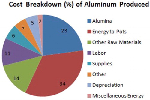
Energy is the product of pot voltage, current and time, and it is energy that has to be paid for, not current. To get an idea of how much the costs with the energy impacts in the final aluminium production cost, let us calculate the energy bill for a regular pot for one year of operations. We have

Using an average line current of 240.000 Amps, an average pot voltage of 4.50 V and a price of US$0.050 per kilowatt-hour, we have

In the context of higher energy prices, reduction of energy consumptions is the top priority and one of the main levers is to reduce the anode-to-cathode distance (ACD) and thereby improve the overall energy efficiency of the cell (Welch, 1999). To keep an optimal ACD, the process control computer adjusts the ACD based on the analog data received from the process control hardware interface. The reliability of the data measurement is fundamental to meet the ACD requirements for a lower energy consumption. In the present work, we want to improve the pot energy consumption by using a state-space observer based on Kalman filtering to generate pot resistance estimates to be used by the control system to adjust the ACD distance.

1.1. Overall progress on control solutions

The status of the currently prevailing control technologies of the industries is well developed and widely accepted. They are readily accessible to any new procedures and are adaptable in various areas of knowledge. Next, some of the latest control solutions are presented that employ Kalman filtering to resolve different control problems in different areas of knowledge.

Kalman filters are applied to a wide variety of scenarios in the general industry including the fusion of measurements that are corrupted by noise. The developments and applications of Kalman filters have evolved to a very high state-of-the-art method for state estimation for dynamical systems, which could be described by difference or differential equations, especially in state-space form. Such Kalman filter combinations aid to improve the performance of the overall system and have attracted the growing interest of researchers in various scientific and engineering areas due to the growing need of adaptive intelligent systems to solve the real-world problems. In general, the various approach solutions try to map input patterns to appropriate output patterns. The learning methods work in such a way to improve the desired mapping between input and output patterns, which is the common objective (Ouyang, Lee, & Lee, 2005). The problem of finding a suitable model structure and a particular parameterizations in order to describe the input–output behaviour of a given unknown system is the realm of the system identification.

Hestetun and Hovd (2006) propose measurements of the current through anodes in different parts of the cell, in order to estimate states and parameters using an extended Kalman filter (EKF). Hsieh and Wang (2011) present an EKF to estimate the NO concentration, from the optic of association with our proposal; the EKF is the software element of an indirect measurement system, the experimental results show that the EKF-based approach can significantly improve the accuracy of NO concentration measurements from the original NO sensor. An unscented version of the KF approach is developed in Chen and Yu (2014), with a novel hybrid modelling method for short-term wind speed forecasting. The proposed approach is compared to several conventional methods for short-term wind speed prediction. Meau, Ibrahim, Narainasamy, and Omar (2006) report the development of a hybrid system consisting of an ensemble of EKF-based multi-layer perceptron network and a one-pass learning fuzzy system for the recognition of electrocardiogram signals. The work in Xu, Wang, and Chen (2012) is based on a novel EKF to estimate the state of charge based on a stochastic fuzzy neural network battery model.

Scientific investigation on the properties of KF, statistics and computational intelligence approaches, such as investigations on stability and computational complexity, can be seen in de Jesús Rubio and Yu (2007), Barragán, Al-Hadithi, Jiménez, and Andújar (2014), Castañeda and Esquivel (2012), Juang, Lin, and Tu (2010), Muralisankar and Gopalakrishnan (2014) and Majid, Taylor, Chen, and Young (2011). In de Jesús Rubio and Yu (2007), an EKF is applied to train state-space recurrent neural ANN for non-linear system identification. In order to improve the robustness of the EKF algorithm, dead-zone robust modification is applied. The Lyapunov method is used to prove that the EKF training is stable. In Barragán et al. (2014), the authors present an online Takagi–Sugeno fuzzy modelling general methodology that is based on the EKF; the methodology works online with the system and is very efficient computationally in the presence of noise.

This paper is organized in five parts. The first part presents relevant relationships between the energy consumption and the resistance control for the aluminium cell. The second part reviews the resistance control principles and how it regulates the energy for an individual pot, focusing the relationship between the ACD and the pot voltage. The third part is dedicated to the plant model and state observer design based on the Kalman filtering approaches. The fourth part explains the Kalman filter tunings for the resistance control with real data. Lastly, the fifth part presents the final commentaries and conclusion remarks about the present study.

2. Energy control for aluminium production cell

The main objective of this section is to make a contextualization of the energy control in the aluminium production cell. It presents the mapping of input and output process control variables, outlining the importance of the resistance control to keep the energy consumption in the desired levels for the pot and potline operations. The process control is modelled as a closed-loop system.

2.1. The anode-to-cathode distance

The ACD in the Hall–Héroult cell is the distance from the lower surface of the carbon anode to the top surface of the aluminium metal pad. Decreasing the ACD lowers the voltage and energy requirements of the cell (Green, 2007; Solheim, 2014; Ying-fu, 2011). The ACD must be large enough to ensure that the liquid metal does not contact the anode and short circuit the cell. A reference target resistance (or target voltage) should be set to match a required ACD. The control of the ACD is critical to maintain the cell stability, in regulation of the heat balance and in achieving efficient production levels (current efficiency, energy consumption and anode consumption). This control is achieved by automatic adjustment of the anode bridge in response to the cell resistance signal. As such, the ACD for individual anodes will vary depending on the resistance of each anode assembly, which may be affected by many factors such as anode quality, the actual anode area and the resistance of the electrical connections.

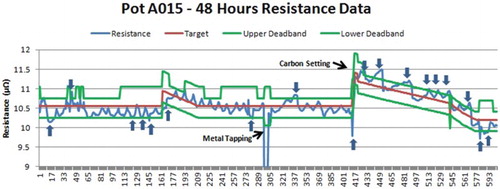
Figure 2 shows the process computer in action to maintain the pot resistance within the resistance target deadbands so that the pot can operate in a pre-defined ACD (Hanusa, 2015). Because the anodes are consumed, the anode beam, which is holding all the anodes in position, has to be gradually lowered downward into the cell to maintain a constant anode–cathode distance. This task is performed by the process computer that uses the pseudo-resistance as a reference to make the decision to adjust the beam. In that sense, one particular ACD value is related to a particular pot voltage (resistance) target. The pot resistance from each pot is continuously varied in response to variations in the anode voltage and the process control system will try to keep the ACD distance by issuing down bridge movements (lowers) and up bridge movements (raises) to maintain the pot resistance within the desired resistance deadband (or desired ACD).

Figure 2. Resistance control: bridge movements to keep ACD.

Operation at too high-voltage wastes electrical energy as heat and eventually raises the temperature on the pot, which in turn leads to lower current efficiency (Green, 2007). On the other hand, operation at too low voltage squeezes the ACD with the consequence of low current efficiency. This low-voltage operation also over-cools the pot and is disruptive to the heat balance, with the end result being a noisy pot and a long-term cyclic operation. Voltage must be controlled with consequences of operation at too high voltage and at too low voltage in mind in order to achieve the highest level of efficiency (Totten & MacKenzie, 2003).

2.2. Pot resistance control

The pot voltage can be classified into three components (Haupin, 1992; Tarcy & Tørklep, 2005; Tarcy, Gavasto, & Ray, 1986; Tarcy, Kvande, & Tabereaux, 2011).

• The electrochemical component (sometimes called electrode voltage) that is essentially independent of the ACD and non-linearly dependent upon the alumina concentration, current density and cell temperature.

• The Ohmic or resistive component (sometimes called the ACD voltage) that is essentially independent of the electrode.

• The battery component (BEMF) that is essentially a fixed voltage independent of amps. It is not shown in Figure 3.

Figure 3. Dependence of the pot voltage component on ACD.

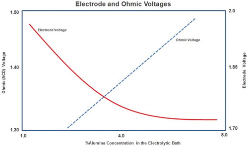
Summing up the first two components gives the total voltage across the cells bath (between anode and cathode) minus the BEMF . The sum represents the quantity that is affected when the cells alumina concentration changes. The other voltage components (externals, voltage drop, cathode drop, etc.) are essentially constant with respect to the alumina concentration changes (Taylor, Chen, & Young, 2013).

Pot resistance, not the pot voltage, is actually used to control the energy consumption in the pot. There is a relationship between resistance and voltage that makes use of resistance necessary to control the pot. When the potline amperage is turned off, the pots still have some residual voltage that is usually referred to as the battery effect or back emf (BEMF). This battery effect is independent of current while both the electrode voltage and the ohmic voltage depend on current. In order to control the energy consumption inside the pot, a pseudo-resistance is used as a control metric because it nearly eliminates the signal fluctuations due to changes in line load. Subtracting the BEMF negates the ‘battery effect’ of the Hall cell, leaving the pure resistance through the pot's externals, cathode, anodes and bath. While the line load and pot voltage fluctuate over time, the cell's pseudo-resistance remains virtually unchanged. The pseudo-resistance is calculated by Ohm's law from pot volts and line current, after back emf is subtracted from the pot volts (Burkin, 1987; Donaldson & Raahauge, 2013): (1) where is the calculated electrical resistance, is the pot voltage, BEMF is the battery effect voltage and is the line current.

With Equation (1(1) ), the typical line current fluctuation effects can be eliminated, which allow the electrical resistance to be used to control both the alumina concentration and ACD. The alumina feed control is designed to maintain the pot within a desired alumina concentration range by exploring the relationship between the alumina concentration change rate and the pot resistance variation as in Equation (1(1) ), but alumina feed control is not in the scope of this present work. We want to explore the resistance control.

The resistance control is designed to keep each cell's ACD at an optimum level, balancing the need to run a stable metal pad with the absolute requirement of thermal stability (Donaldson & Raahauge, 2013; Taylor et al.,2013):

• ACD at a critical base value needed to ensure operating stability and the necessary heat input.

• Modifiers above the ideal base resistance target needed on a temporary basis to handle instability resulting from transient events such as metal tapping, anode setting or temporary upset of the metal pad. The difference between the actual pot resistance and the target resistance is calculated and the appropriate move decision made.

The resistance control changes the ACD distance by moving the anode bridges in the pot. The bridge move decision is taken considering the different process control statuses triggered by the normal pot operations, such as metal tapping, carbon settings and bath additions, as shown in Figure 2. Each point in the graph represents a five-minute pot resistance average (blue line). Every five-minute average is compounded by 1500 readings of individual pot resistance value. The pot resistance information is the main input from the hardware interface, and from the process computer perspective all control actions regarding the ACD adjustment are dependent on the pot resistance value.

In many occasions, the quality of the hardware interface signals provided biased pot voltage and line current values to the process control programs, which is reflected in the pot resistance. Biased signals hide serious control problems, can harm significantly a pot in a short-term period and can lead to total loss if it is not identified and fixed in a medium term. Adding or removing power to the pot is always a control action based on the pot resistance behaviour over the time.

Due to the dynamic nature of the aluminium cell, a series of temporary resistance(voltage) modifiers are programmed to keep the optimum ACD distance. These modifiers are used around various events to stabilize the metal pad or to add heat to the cell. The resistance modifiers take a very important role on the final pot voltage. The main resistance modifiers are the ones due to noisy conditions that will be seen next.

2.3. Pot noise control

The resistance control has a very important module called the noise control. In the aluminium industry, the term noise is a general measure of the variability of the pseudo-resistance signal over a relative short period of time. Noise can be measured by a variety of metrics including absolute maximum to minimum, also called peak-to-peak noise (PPN), calculated every three or five minutes (Taylor et al., 2013; Jin & Lin, 2012). (2) where is the noise value, and are the maximum and minimum resistance values in a specific short period time, respectively. In general, the smelter hardware interfaces are able to sample the pot resistance (pot voltage and line current) in a frequency rate of 200 ms (or five times a second), which represents a total of 900 readings (three minutes noise calculation) or 1500 readings (five minutes noise calculation).

The purpose of noise control is to allow a pot to run at the minimum ACD that can be achieved by maintaining the stability of the pot (Bearne, 1999). In terms of resistance control, the noise value is the main metric of the pot stability and that happens to be a very good assumption since the pot operational stability is a function of two pot conditions:

• Magnetics: a function of the size of the vertical magnetic field in the pot governed by the bus design and overall current intensity of the potline.

• Horizontal currents in the metal: a function of bottom conditions governed by muck, bottom ridge and anode current distribution.

It is very common for a noisy pot to fall into the second condition after an anode setting when the anode rod positions are adjusted . Bad rod adjustments lead to an unbalancing current distribution on the pot and reflects in the pot resistance. Noise control can only affect instability caused by horizontal currents in the metal (McGraw et al., 1989; Bearne, 1999). Ideally, the pot has no bottom deposits (excess of alumina or muck). There are only two options for stopping the noise:

• Increase the metal: an increase in the mass of metal in the pot increases the amount of force needed to amplify the wave.

• Increase the ACD: a big enough increase in the overall ACD diminishes the local decreases in ACD caused by a heaved metal pad, in turn diminishing the amount of horizontal equalizing currents and the resulting magnetic forces.

Although an increase in the amount of metal can be a viable option for long-term noise problems in some situations, the only viable short-term solution is an ACD increase. Noise control works by increasing the ACD through the use of temporary resistance modifiers whenever the pot becomes unstable (noisy) and by removing these resistance modifiers when the pot becomes sufficiently stable (quiet) (Taylor et al., 2013; Cauvin, Goodnow, & Simard, 1974). Figure 4 shows the pot resistance and pot noise behaviour along 12 hours. There are two key things to make the stability (noise) control to succeed:

Figure 4. Noisy Pot Behaviour.

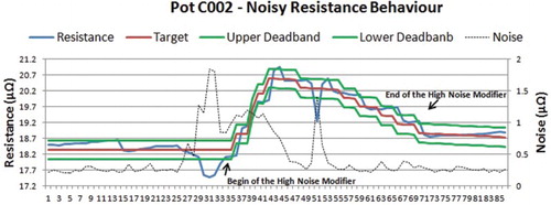
• Addition of a large enough resistance modifier (extra voltage) to make sure the pot becomes stable.

• Verification for a long enough period of time that the pot is stable before attempting to ramp off (remove) the extra voltage.

The addition and the removal of the resistance modifier will follow trigger values specified by operational and process people in the process control computer. If a noisy condition is persistent even after the extra resistance modifier, then the operational staff has to go in the pot and check for bad anode rod adjustments or the existence of burn-offs (fallen anode pieces) inside the electrolytic bath.

3. Kalman filters tuning for resistance control

In our approach, the filter design is oriented to measure the state variables of the production cell. The goal is to compute a set of filter gains that represents real (or much closer as possible) behaviour of the pot resistance in the electrolytic bath, which is an observable system. The design and analysis of the Q and R covariance matrices are performed to establish the best filter tuning for the pot resistance estimate (Braga, Fonseca, Nagem, Farid, & Silva, 2008; Miloudi & Draou, 2001; Neto, Farid, & deAbreu, 2010; Pinho & da Silva Tavares, 2009; Van Der Merwe, 2004; Wan & Van Der Merwe, 2000).

3.1. The plant model

The plant model is described in the state space that has the canonic representation given by (Braga et al., 2008; Yeh, 1990) (3) (4) where represents the electrical resistance, slope and curvature. The output represents the measured signal. represents the system dynamics, is the related noise output. and are the zero mean Gaussian white noise sequences with Q and R known variances, respectively.

3.2. The state observer design

The state observer's main purpose is the replacement of a conventional measurement system by a device based on hardware and software. The observer has two main issues that are the pot (plant) state estimation and gain adjustment. The use of a state observer is related to the existence of noisy measurements, hard access and high cost of sensors (Smith, Monti, & Ponci, 2007). The observer dynamic is given by (5) where is the proportional gain that can be computed using deterministic or stochastic methods. In this approach, the gains are computed by KF and the system is driven by noise.

The EKF and unscented Kalman filter (UKF) theories' references that base this work can be found in Bozic and Chance (1998), Welch and Bishop (1995), Welch (2014), Yeh (1990), Pinho and da Silva Tavares (2009), Miloudi and Draou (2001), Wan and Van Der Merwe (2000), Van Der Merwe and Wan (2001), Van Der Merwe (2004), Fonseca, Oliveira, Abreu, Ferreira, and Machado (2013), Pedrycz and Gomide (1998), Pedrycz and Peters (1998), Romanenko and Castro (2004), Kandepu, Foss, and Imsland (2008), Mouzinho et al. (2005) and LaViola Jr. (2003).

3.3. The control law of the process

The purpose of the process control computer system in the aluminium production is to regulate the amount of alumina (raw material) and electricity required by each production cell (pot) during the electrolysis process. The metal amount produced is dependent on the electrical current and pot current efficiency. This relationship is based on the Faraday Law (Zhuk, Sheindlin, Kleymenov, Shkolnikov, & Lopatin, 2006). According to the Faraday Law, the maximum aluminium amount that can be produced by the electrolysis process is 8.053 kg per kiloampere (kA) in a period of 24 hours. With that, a formal relationship can be built for the aluminium production, . (6)

The relationship between these two operators are mapped into the function and based on Faraday Law. (7) where is the current efficiency expressed in percentage (%) and I is the line current intensity expressed in kiloampere (kA). To be considered efficient, the process computer should be able to deliver the correct alumina amount and power (energy) to match the line current intensity provided to the aluminium electrolysis process. The objective is to achieve the maximum aluminium production to a given line current intensity. The knowledge of the operating voltage of the cell is required when the energy consumption (EC) is taken into account. If the current efficiency and the pot voltage are known, then we can describe the control law of the process by (8)

In Equation (8(7) ), the operational cell voltage given is in volts (V), and the current efficiency given as a fraction (not in per cent). EC is expressed in kWh per kg aluminium and represents the best technological parameter in aluminium production, because it also includes current efficiency (Kvande & Drabløs, 2014; Luo & Soria, 2007).

Pot voltage is linked via the bath resistance to the ACD. A low pot voltage calls, therefore for a small ACD. It is therefore desirable to operate at a high current efficiency and consume as little voltage as possible at the same time.

3.4. Estimation and control

One particular drawback about observers is that they are not straightforward to design for systems having more than one measurement. Even though the pot resistance comes from the line amps and pot voltage, it represents the only input to our observer model (Figure 5).

Figure 5. Kalman filter state observer.

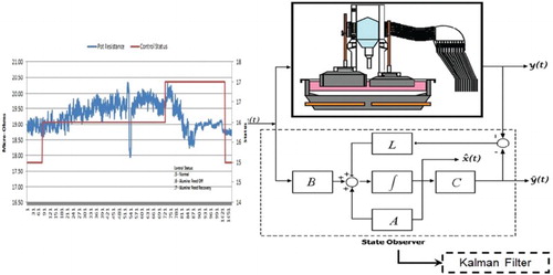
If the model is perfect the output will be equal to the input (the real resistance). In practice, there will be a difference between the real measurement and the estimated measurement (9)

The error e is used to update the estimate via the Kalman filter gain, K. Thus, the correction of the estimates is error driven, which is the same principle as that of an error-driven control loop.

3.4.1. Estimation and control using EKF.

The numerical value of the observer gain determines the strength of the correction. The EKF gain tuning was performed by using the duality principle of the Q and R matrices, following the guidelines in Yeh (1990).

The main purpose of the EKF gain adjustment method via Q and R matrices manipulation was to observe its effect on the estimated pot resistance, proving that the filter is sensitive to real voltage variation on the pot. Given Q and R as the noise covariance matrices for the process and for the measurement, respectively. For the filter gain adjustments, three scenarios were considered: (10a) (10b) (10c)

Having these three possible scenarios, (10a(9) )–(10c(10c) ), for the EKF gain adjustment, the first scenario (rule 1) was preferred to run the heuristics for the filter tuning. For that purpose, the R matrix values were kept unchanged, while the Q covariance matrix values were modified. The resulting variations were associated with the Kalman filter bandwidth and filter stability (11)

Following the control procedure outlined in Braga et al. (2008), Bozic and Chance (1998) and Ferreira and Luis (2003), the filter tuning method employed the parameter adjustments in such a way to allow the passage of frequency ranges that affects the pot resistance.

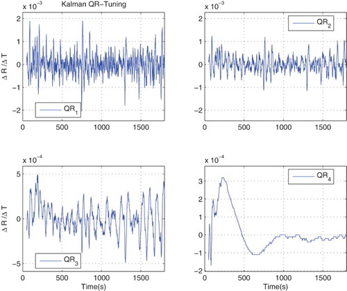
Figure  6(a) presents the matrices deviation due to QR rule, relation (10a(9) ), with weighting matrices by keeping R constant and varying Q. The element variations are used to verify the gain order related to a specific frequency range and determine the pattern that best represents the pot resistance variation. The filter gains associated are presented in Figure  6(b), with Kalman filter gains as a result of the QR duality principle application. Note that the gain values are reduced, following relation (11(10a) ).

Figure 6. EKF fine tuning following the QR duality principle.

The QR relation values for cases 1–4, Figure  6(c), are the same for the elements of matrices Q and R, and were defined by the process specialist as being , and , and their correspondent values are in the order of .

For normal pots, the results of the heuristic using EKF can be observed in Figure 7.

Figure 7. EKF: QR adjustment with off-line data using Matlab – Rule 1.

During the tests, the EKF gain (K) was low and dependent on the initial high Q elements mainly. Higher Q elements allowed better fit during the test with dynamic conditions, but lead to higher noise before achieving the filter convergence. On the other hand, lower Q variance did not allowed a good dynamic tracking. A trade-off between such conditions had to be found during the filter tuning.

For our specific field of study, the pot resistance, the measurement and state estimation transition model are non-linear. The linear and quadratic transformation were not able to produce reliable results because the error propagation in noisy pots (high variation in the measurements) could not be well approximated by a linear or a quadratic function, and as a consequence the EKF performance was poor in those pots, with cases where the estimates have diverged altogether. By using a second-order EKF, the error propagation did not get any better when the pot resistance changed abruptly.

3.4.2. Estimation and control using UKF.

A sensitivity analysis for UKF fine tuning was performed, starting from the same state and measurement model used for EKF implementation. Different test trials were performed first in an off-line state using batch data in the process computer, and afterwards with dynamic and real conditions to determine suitable values for the filter design parameters. The analyses were performed using the real resistance, the EKF estimates, the UKF estimates and the current resistance value used for control by the process computer, using the gain adjustments represented by (10b(10b) ) and (10c(10c) ).

To define R and matrix values the variance values in the range of – were considered suitable for a good filter convergence. Typical initial state covariance matrix was used, ranging from to . Very fair values were obtained during sensitivity analysis under dynamic conditions when Q variances between and were used.

The true and estimated states using UKF and EKF are shown in Figure 8. Both filters were applied to normal pots and to noisy pot during the period of tests.

Figure 8. Real and estimated measurements.

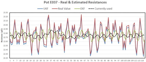
The real data in the Figure 8 demonstrate that the existing current filter (dotted line) used to control the pot is very little sensitive to large resistance variations, while EKF (green line) and UKF (blue line) resistance estimates were much closer to the real value (red line). In that sense, for the process computer control, both EKF and UKF estimated states represented a more reliable reference to the process computer than the existing(current) filter.

In the world of the aluminium production, a cell with high resistance variation receives the technical jargon of noisy pot. A general process control practice in the aluminium industry is to treat noisy pots (no matter if it is a drop or a peak in the resistance) by making small additions of extra voltage to the cell in order to keep the desired ACD. These voltage amounts tend to increase along the time if the problem persists. The process computer performs the extra voltage addition automatically, based on the pot noisy trigger values(as depicted in Figure 9) previously specified by the operational and process teams. The pot resistance information captured from the hardware interface is checked against those triggers constantly. Thus, the quality of the pot resistance signal to perform a good pot control is extremely important. Noisy measurements will lead the process computer to take wrong decisions, sometimes adding unnecessary extra voltage to the cell, sometimes delaying to react to a problem. Some constraints were implemented on the computer algorithm so that the filter resistance estimates could not go too far. The constraints are to avoid the system to use bad estimates if they happen. Bad estimates can be caused by an error on the real pot resistance signal. Errors in the hardware devices in the field can cause impossible pot resistance values treated as real values by the system. We have not seen any case where the true states violated the constraints.

Figure 9. EKF and UKF: resistance estimates errors.

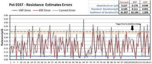
The purpose of the observer is to estimate assumed unknown states in the model. The model errors are calculated using the real value and the estimated value as shown below: (12)

The performance of the two filters was compared using the absolute estimate as in Equation (12(10b) ), which represents how far the two filters were from the real value.

After checking if the observer was producing usable estimates, the next step was to measure how close the EKF and UKF resistances were from the real value. The absolute error shown in Figure 9 makes clear the influence of the noise in the state estimates. EKF estimates carried a considerable amount of noise, while the UKF estimates had a flat pattern on the absolute error with a small difference from the real value.

The purpose of the research is to develop a new resistance control to improve the overall energy cost in a pot. The Absolute Error in Figure 9 represents the most significant information for the process computer to decide about the best time to add or to remove extra voltage from the production cell. Along the period of tests, there were many cases where the old resistance control system had failed to take the correct decision on noisy cells. The Standard Deviation and the Coefficient of Variation were calculated over the Absolute Error and they have shown that the variability was smaller when UKF resistance estimates were used.

The test results supported the hypothesis that the dynamic performance of UKF estimates is better when compared with the EKF estimates in non-linear environments although there were extremely noisy pots (i.e., with fallen anodes inside the bath, bad wiring, low liquid level, beam problems) where the UKF was not able to converge. In the field, from operational perspective, excessive noisy cells need manual intervention of plant personnel since the process computer is not expected to fix operational issues.

Both EKF and UKF estimates were much closer to the real pot resistance value when compared to the existing filter that have been used to take control actions in the pot, as depicted in Figure 8.

What do these test results mean to the purpose of controlling the energy consumption in the pot?

• The quality of the estimate is inversely proportional to the state estimates errors (e). So, the smaller e, the best is the resistance estimate. In Figure 9 the 0 (zero) means that the estimated resistance matches the real resistance value. For the resistance control objective, it really does not matter if the difference is positive or negative, that is the reason the estimated error is shown as an absolute value in the graph. As explained in Section 2.3, the resistance variation is the main drive for control actions in the pot (add/remove extra voltage, bridge movements).

• The EKF state estimates contained too much noise, producing a high estimate error. The high error was an important drawback of the EKF estimates. Using EKF resistance estimates as input to the resistance control would add a significant unnecessary amount of extra voltage to the pot because the control system uses the PPN noise to add and to remove voltage automatically from the pot, as explained in Section 2.3. The trigger to add extra voltage to the pot would be activated six times if the EKF resistance had been used.

• The UKF resistance estimates had gotten much smaller state estimate errors, carrying out a minimum amount of noise. If UKF had been used the extra voltage trigger would not have been activated. The old (existing) resistance estimate had triggered the extra voltage limit 19 times.

• In a normal control scenario, when the extra voltage trigger limit is fired the computer will add the extra voltage to the pot until the resistance variation falls below a certain value, then the extra voltage is removed. It is necessary to stay a certain time above the limit to start the extra voltage, as it is necessary to stay a minimum time below the limit to remove the extra voltage.

• Based on the test results, the decision was to use UKF as the state-space observer for all pots.

4. Concluding remarks

In this paper, a novel formulation of the energy consumption control in an aluminium production cell was presented. The main principles of EKF and UKF for state estimation were discussed, as well as the differences between the two approaches. A filter tuning procedure based on the manipulation of the Q and R matrices was described. A scaled EKF and UKF filters have been designed and implemented in a process control computer using real data and taking control actions based on the state estimations. A procedure to include constraints in the code was developed and impossible or out of context state estimates were clipped in the program. The overall results had shown that both EKF and UKF resistance estimates were much closer to the real values when compared to the old resistance estimate method used in the process control, with UKF representing the best filter choice to perform the new resistance control. Relevant Kalman filter parameters (Q and R variances, Kalman gains, UKF scaling parameters) had been selected after finding the best filter tunings.

The best UKF performance was due to the increased time-update accuracy and the improved covariance accuracy. Especially in noisy pots the UKF performance was substantially better in long-term state estimation error.

The energy control inside the pot relies on the accuracy of the resistance estimate. Actually, the electrical resistance is the only real-time data input for the process control system. Poor resistance estimates lead to wrong decisions by the resistance control modules and can result in a total loss of the production cell. The UKF resistance estimate can contribute to a significant improvement on the pot resistance control (and noise control) by providing a better approximation of the real resistance which will help to achieve the goals of the process engineers and operational teams.

Acknowledgments

The authors gratefully acknowledge the support from the Postgraduate Program in Electrical Engineering of the Universidade Federal do Maranhao (PPGE/DE.EE/UFMA) in Brazil.

Disclosure statement

No potential conflict of interest was reported by the authors.

ORCiD

Carlos Augusto P. Braga http://orcid.org/0000-0001-8081-0270

Joao Viana da Fonseca Netto http://orcid.org/0000-0003-4606-7510

References

- Barragán, A. J., Al-Hadithi, B. M., Jiménez, A., & Andújar, J. M. (2014). A general methodology for online TS fuzzy modeling by the extended Kalman filter. Applied Soft Computing, 18, 277–289. doi: 10.1016/j.asoc.2013.09.005
- Bearne, G. P. (1999). The development of aluminum reduction cell process control. Journal of the Minerals, Metals & Materials Society, 51(5), 16–22. doi: 10.1007/s11837-999-0035-5
- Bozic, S. M., & Chance, R. (1998). Digital filters and signal processing in electronic engineering: Theory, applications, architecture, code. Chichester: Elsevier.
- Braga, C., Fonseca, J., Nagem, N., Farid, J., & Silva, F. (2008). Kalman filter for indirect measurement of electrolytic bath state variables: Tuning design and practical aspects. Sensors and Transducers Journal, 90, 139–149. Retrieved from http://www.sensorsportal.com/HTML/DIGEST
- Burkin, A. (1987). Production of aluminium and alumina. Critical reports on applied chemistry (Vol. 20). Published on behalf of the Society of Chemical Industry by Wiley, Chichester. Retrieved from https://books.google.com/books?id=949TAAAAMAAJ
- Castañeda, C. E., & Esquivel, P. (2012). Decentralized neural identifier and control for nonlinear systems based on extended kalman filter. Neural Networks, 31, 81–87. doi: 10.1016/j.neunet.2012.03.005
- Cauvin, S., Goodnow, W., & Simard, J. (1974, May 21). Control of an aluminum reduction cell. Google Patents. Retrieved from https://www.google.com/patents/US3812024 (US Patent 3812024).
- Chen, K., & Yu, J. (2014). Short-term wind speed prediction using an unscented Kalman filter based state-space support vector regression approach. Applied Energy, 113, 690–705. doi: 10.1016/j.apenergy.2013.08.025
- de Jesús Rubio, J., & Yu, W. (2007). Nonlinear system identification with recurrent neural networks and dead-zone Kalman filter algorithm. Neurocomputing, 70(13), 2460–2466. doi: 10.1016/j.neucom.2006.09.004
- Donaldson, D., & Raahauge, B. E. (2013). Essential readings in light metals. Volume 1, Hoboken, NJ: Wiley. Retrieved from http://public.eblib.com/choice/publicfullrecord.aspx?p=3058927http://public.eblib.com/choice/publicfullrecord.aspx?p=3058927.
- Ferreira, C. C. T., & Luis, S. (2003). Alocacao de autoestrutura utilizando controle robusto LQG/LTR e computacao evolutiva (Master's thesis). Universidade Federal do Maranhao-UFMA, Brazil.
- Fonseca, J. V., Oliveira, R. C., Abreu, J. A., Ferreira, E., & Machado, M. (2013). Kalman filter embedded in FPGA to improve tracking performance in ballistic rockets. Paper presented at Computer modelling and simulation (UKSim), 2013 UKSim 15th International Conference on (pp. 606–610).
- Green, J. A. (2007). Aluminum recycling and processing for energy conservation and sustainability. Ohio: ASM International.
- Hanusa, T. P. (2015). The lightest metals: Science and technology from Lithium to Calcium. Chichester, Wiley.
- Haupin, W. (1992). The liquidus enigma. In G. Bearne, M. Dupuis, & G. Tarcy (Eds.), Essential readings in light metals: Aluminum reduction technology (Vol. 2, pp. 804–807). Hoboken, New Jersey: Wiley.
- Hestetun, K., & Hovd, M. (2006). Detection of abnormal alumina feed rate in aluminium electrolysis cells using state and parameter estimation. Computer Aided Chemical Engineering, 21, 1557–1562. doi: 10.1016/S1570-7946(06)80269-5
- Hsieh, M.-F., & Wang, J. (2011). Design and experimental validation of an extended Kalman filter-based NO concentration estimator in selective catalytic reduction system applications. Control Engineering Practice, 19(4), 346–353. doi: 10.1016/j.conengprac.2010.12.002
- Hyland, M. (2015). Light metals. Hoboken, NJ: Wiley. Retrieved from https://books.google.com/books?id=FijWBgAAQBAJ.
- Jin, D., & Lin, S. (2012). Advances in future computer and control systems (Vol. 1). New York: Springer.
- Juang, C.-F., Lin, Y.-Y., & Tu, C.-C. (2010). A recurrent self-evolving fuzzy neural network with local feedbacks and its application to dynamic system processing. Fuzzy Sets and Systems, 161(19), 2552–2568. doi: 10.1016/j.fss.2010.04.006
- Kandepu, R., Foss, B., & Imsland, L. (2008). Applying the unscented kalman filter for nonlinear state estimation. Journal of Process Control, 18(7), 753–768. doi: 10.1016/j.jprocont.2007.11.004
- Kvande, H., & Drabløs, P. A. (2014). The aluminum smelting process and innovative alternative technologies. Journal of Occupational and Environmental Medicine, 56(5 Suppl.), S23–S32. doi: 10.1097/JOM.0000000000000062
- LaViola Jr, J. J. (2003). An experiment comparing double exponential smoothing and Kalman filter-based predictive tracking algorithms. Paper presented at the VR (Vol. 3, p. 283). Brown University Technology Center for Advanced Scientific Computing and Visualization; Providence, RI, 02912, USA.
- Luo, Z., & Soria, A. (2007). Prospective study of the world aluminium industry (JRC Scientific and Technical Reports. EUR 22951).
- Majid, N. A. A., Taylor, M. P., Chen, J. J., & Young, B. R. (2011). Multivariate statistical monitoring of the aluminium smelting process. Computers & Chemical Engineering, 35(11), 2457–2468. doi: 10.1016/j.compchemeng.2011.03.001
- McGraw, W., Christian, K., Hall, W., Miller, G., Seaman, C., & Kozarek, R. (1989, March 21). Estimation and control of alumina concentration in Hall cells. Google Patents. Retrieved from https://www.google.com/patents/US4814050 (US Patent 4,814,050).
- Meau, Y. P., Ibrahim, F., Narainasamy, S. A., & Omar, R. (2006). Intelligent classification of electrocardiogram (ECG) signal using extended Kalman filter (EKF) based neuro fuzzy system. Computer Methods and Programs in Biomedicine, 82(2), 157–168. doi: 10.1016/j.cmpb.2006.03.003
- Miloudi, A., & Draou, A. (2001). Neural controller design for speed control of an indirect field oriented induction machine drive. Paper presented at the The 27th annual conference of the IEEE Industrial electronics society, 2001. IECON'01. Vol. 2 (pp. 1225–1229).
- Mouzinho, L., Neto, J. F., Luciano, B., Freire, R., Barros, J. D. J., & Fontgalland, G. (2005). Kalman filter in real time for indirect measurement of space vehicle position using a reconfigurable architecture. Paper presented at 2005 IEEE instrumentation and measurement technology conference proceedings, Ottawa, ON, Canada. (Vol. 2, pp. 853–858).
- Muralisankar, S., & Gopalakrishnan, N. (2014). Robust stability criteria for Takagi–Sugeno fuzzy Cohen–Grossberg neural networks of neutral type. Neurocomputing, 144, 516–525. Retrieved from http://www.sciencedirect.com/science/article/pii/S0925231214006006. doi: 10.1016/j.neucom.2014.04.019
- Nappi, C. (2013). The global aluminium industry: 40 years from 1972. London, International Aluminium Institute [online]. Retrieved from http://www.world-aluminium.org/publications.
- Neto, J. V. F., Farid, J. A., & de Abreu, J. A. P. (2010). Qr-duality tuning of standard kalman filters oriented to rocket velocity indirect measurement. Paper presented at the 12th international conference on Computer modelling and simulation (UKSim) (pp. 74–79). Cambridge, UK.
- Ouyang, C.-S., Lee, W.-J., & Lee, S.-J. (2005). A tsk-type neurofuzzy network approach to system modeling problems. IEEE Transactions on Systems, Man, and Cybernetics, Part B (Cybernetics), 35(4), 751–767. doi: 10.1109/TSMCB.2005.846000
- Pedrycz, W., & Gomide, F. (1998). An introduction to fuzzy sets: Analysis and design. Cambridge, UK: MIT Press.
- Pedrycz, W., & Peters, J. F. (1998). Computational intelligence in software engineering (Vol. 16). Singapore: World Scientific.
- Pinho, R. R., & da Silva Tavares, J. M. R. (2009). Comparison between Kalman and unscented Kalman filters in tracking applications of computational vision. Paper presented at VipIMAGE 2009-II ECCOMAS thematic conference on computational vision and medical image processing, Porto, Portugal.
- Romanenko, A., & Castro, J. A. (2004). The unscented filter as an alternative to the EKF for nonlinear state estimation: A simulation case study. Computers & Chemical Engineering, 28(3), 347–355. doi: 10.1016/S0098-1354(03)00193-5
- Smith, A. H. C ., Monti, A., & Ponci, F. (2007). Indirect measurements via a polynomial chaos observer. IEEE Transactions on Instrumentation and Measurement, 56(3), 743–752. doi: 10.1109/TIM.2007.894914
- Solheim, A. (2014). Current efficiency in aluminium reduction cells: Theories, models, concepts, and speculations. Light Metals, 2014, 753–758.
- Tarcy, G. P., Gavasto, T. M., & Ray, S. P. (1986, November 4). Electrolytic production of metals using a resistant anode. Google Patents (US Patent 4,620,905).
- Tarcy, G. P., Kvande, H., & Tabereaux, A. (2011). Advancing the industrial aluminum process: 20th century breakthrough inventions and developments. JOM, 63(8), 101–108. doi: 10.1007/s11837-011-0120-4
- Tarcy, G. P., & Tørklep, K. (2005). Current efficiency in Prebake and Søderberg cells. In G. Bearne, M. Dupuis, & G. Tarcy (Eds.), Essential readings in light metals: Aluminum reduction technology (Vol. 2, pp. 211–216). Hoboken, NJ: Wiley.
- Taylor, M. P., Chen, J. J., & Young, B. R. (2013). Control for aluminum production and other processing industries. Boca Raton: CRC Press.
- Totten, G. E., & MacKenzie, D. S. (2003). Handbook of aluminum: Vol. 1: Physical metallurgy and processes, Vol. 1. New York: CRC Press.
- Van Der Merwe, R. (2004). Sigma-point Kalman filters for probabilistic inference in dynamic state-space models (Unpublished doctoral dissertation). Oregon Health & Science University.
- Van Der Merwe, R., & Wan, E. A. (2001). The square-root unscented Kalman filter for state and parameter-estimation. Paper presented at 2001 IEEE international conference on acoustics, speech, and signal processing, 2001 (ICASSP'01) (Vol. 6, pp. 3461–3464).
- Wan, E. A., & Van Der Merwe, R. (2000). The unscented Kalman filter for nonlinear estimation. Paper presented at the Adaptive systems for signal processing, communications, and control symposium 2000. AS-SPCC. The IEEE 2000, Dortmund. (pp. 153–158).
- Welch, B. J. (1999). Aluminum production paths in the new millennium. JOM, 51(5), 24–28. doi: 10.1007/s11837-999-0036-4
- Welch, G. F. (2014). Kalman filter. In A. Fossati, J. Gall, H. Grabner, X. Ren, & K. Konolige (Eds.), Computer vision (pp. 435–437). London: Springer.
- Welch, G., & Bishop, G. (1995). An introduction to the Kalman filter (Tech. Rep. 95-041). Chapel Hill, NC: University of North Carolina at Chapel Hill. Retrieved from http://www.cs.unc.edu/welch/kalman/kalmanIntro.html.
- Xu, L., Wang, J., & Chen, Q. (2012). Kalman filtering state of charge estimation for battery management system based on a stochastic fuzzy neural network battery model. Energy Conversion and Management, 53(1), 33–39. doi: 10.1016/j.enconman.2011.06.003
- Yeh, H.-G. (1990). Real-time implementation of a narrow-band Kalman filter with a floating-point processor DSP32. IEEE Transactions on Industrial Electronics, 37(1), 13–18. doi: 10.1109/41.45838
- Ying-fu, T. (2011). Anode-cathode-distance model for aluminium reduction cell and its energy consumption. Light Metals, 2, 009.
- Zhuk, A. Z., Sheindlin, A. E., Kleymenov, B. V., Shkolnikov, E. I., & Lopatin, M. Y. (2006). Use of low-cost aluminum in electric energy production. Journal of Power Sources, 157(2), 921–926. doi: 10.1016/j.jpowsour.2005.11.097