
ABSTRACT
The decomposition of the overall forced response into a steady-state and a transient component can be exploited to find reduced-order models that retain both long-term and short-term characteristics of the original system behaviour. To this purpose, the state-space expressions of the aforementioned components in response to inputs with rational transform are derived. The reduced-order model is then obtained by considering separately the asymptotic and transient terms. The suggested approach is tested on benchmark examples of very high dimension.
1. Introduction
Recently, model reduction methods based on the decomposition of the forced response into a transient and a steady-state component (Dorato, Lepschy, and Viaro, Citation1994) have been proposed with the purpose of generating reduced-order models that retain, at least approximately, some important characteristics of both the transient component, for example, its impulse-response energies and moments, and the asymptotic component in response to particular inputs. Also the interpolation-based moment-matching methods (Antoulas, Beattie, and Gugercin, Citation2010; Astolfi, Citation2010; Bultheel and De Moor, Citation2000) retain the steady-state response to particular inputs but do not even ensure, in their standard version, the preservation of stability. To combine transient features with the retention of at least the static or direct-current (DC) gain and, thus, of the steady-state value in the step response, a variant of the balanced-truncation method (Moore, Citation1981) based on perturbation theory (Kokotovic, Khail, and Reilly, Citation1986) has been suggested, which can be implemented using popular control packages (Chaturvedi, Citation2009). No such (limited) extensions are as yet available for other optimal reduction techniques, such as the Hankel-norm (Glover, Citation1984) and -norm (Antoulas, Citation2005; Krajewski and Viaro, Citation2009; Xu and Zeng, Citation2011; Zeng and Lu, Citation2015) approximation methods. Not even the newly proposed metaheuristic model reduction methods (Desai and Prasad, Citation2013; Ramawat and Kumar, Citation2015; Rana, Prasad, and Singh, Citation2014; Sikander and Prasad, Citation2015) explicitly address the problem of asymptotic accuracy.
The reconciliation of optimal or suboptimal approximation methods with specifications on the asymptotic behaviour could be done in the domain of Laplace transforms (transfer functions). Unfortunately, the transfer-function approach is not suited for the reduction of very high-dimensional systems given in state-space form because the conversion from state-space representation to transfer-function is not numerically robust and cannot be safely applied to systems whose order is greater than a few tens. On the other hand, the test inputs often differ from singularity inputs and can involve, to more advantage, combinations of (possibly complex) exponentials, for example, sinusoids.
To overcome these problems, this paper first expresses the components of the forced response to inputs with arbitrary rational transform in terms of the original state-space representation (Section 2): since, in the time domain, these inputs are linear combinations of functions of the form , with
and
, the state response to this kind of functions is preliminarily determined (Proposition 2.1). The reduced-order model is finally obtained by adding an approximation of the transient component to the original steady-state component (Section 3). Essentially, the contribution of this paper consists in the direct time-domain decomposition of the state response and in the separate treatment of its two components. The suggested approach is tested on a pair of high-order benchmark examples taken from the relevant literature (Chahlaoui and Van Dooren, Citation2005) (Section 4). Possible extensions of the method, with particular reference to its applicability to unstable system, are briefly outlined in Section 5.
2. Decomposition of the forced response
In the following, it is assumed that the original system is linear time-invariant strictly proper and asymptotically stable. Denoting its (minimal) state-space representation by the triplet , its forced state response to a causal input
is given by
(1) As is known, if the Laplace transform
of
is real rational and strictly proper with poles in the closed right half-plane,
can be expressed as a linear combination of real non-decreasing exponentials, possibly multiplied by powers of t and/or, in the presence of pairs of conjugate complex poles, sinusoidal functions. If
is exactly proper (Bernstein, Citation2009), that is, proper but not strictly, an impulsive term is also present, but this case is excluded in the sequel for simplicity. Attention will be limited here to such persistent inputs because this is precisely the kind of signals (including singularity inputs and sinusoids) usually employed to test the system behaviour. Note that, since the system is bounded-input bounded-output stable, no resonance phenomena (interaction between input and system modes Dorato et al., Citation1994) can occur.
By denoting the (possibly complex) poles of a strictly proper by
, the corresponding input
can also be written as a combination of functions that are not necessarily real as
(2) where
is the number of distinct poles of
,
denotes the multiplicity of pole
with
and
. The combination coefficients
in (Equation2
(2) ) are real whenever
is so, and complex otherwise. Also, since the coefficients of
are assumed to be real, if
is a complex pole of
, then its conjugate
is also a pole of
, and the combination coefficient of every function
associated with
is conjugate to the coefficient of the homologous function
associated with
. Under these conditions, in fact, the overall input (Equation2
(2) ) is real for all t. In the sequel, reference is made to this expression of the input because it contains functions of one type only, namely
. By linearity, the forced state response to the general input (Equation2
(2) ) is given by a linear combination of the responses to these basic signals. The following result, whose conceptually simple proof can be found in the Appendix, provides a useful tool for finding the forced response to an input of the general form (Equation2
(2) ).
Proposition 2.1
The forced state response of the asymptotically stable system to the causal input
(3) is given by
(4)
Remark 2.1
The invertibility of the matrix is guaranteed because the eigenvalues of the asymptotically stable matrix A lie in the open left half-plane while
lies in the closed right half-plane.
Remark 2.2
The first term on the right-hand side of relation (Equation4(4) ) contains the exponential function
, which depends on the system modes only. Therefore, this term represents the transient component
of the forced response to the considered input. Instead, the addenda under the summation symbol depend only on the input modes associated with the pole
of the transform
of (Equation3
(3) ) and together form the asymptotic (or steady-state) component
of the response.
Remark 2.3
As Equation (Equation4(4) ) shows, in general the asymptotic component
of the overall forced output response, which is related to the overall forced state response via
(5) is not simply proportional to the input but is a linear combination of the input and its first derivatives.
It is easy to derive from (Equation4(4) ) the forced responses to the singularity inputs, which are reported next for convenience. Precisely, the response to
,
, turns out to be
(6) In particular, the step and ramp responses are, respectively,
(7)
The response to
(8) can be obtained by combining the responses to
and
according to the conjugate coefficients
and
. After some trivial manipulations, this response turns out to be
(9) whose transient and steady-state components can be identified easily.
3. Model reduction
Model reduction is, by its very nature, an input–output problem. Therefore, in the following, attention focuses on the forced output response , simply related to
via (Equation5
(5) ). Its transient and steady-state components are immediately obtained in time domain from the corresponding state components without the preliminary determination of their Laplace transforms, which would entail computing the transfer function
of the high-order original system and expanding
into two partial fractions, one with the denominator of
(transient component) and the other with the denominator of
(steady-state component). It follows that the approximation of the transient component can be carried out by referring directly to the triplet of matrices of its state-space realization, which is easily determined from the state responses in Section 2.
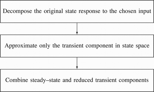
According to the approach outlined in Section 1, the suggested reduction procedure can be presented as follows.
Procedure 3.1
Determine the transient and asymptotic responses of the original system to the chosen test input from its state-space representation
and take the state-space realization
Approximate
Form the reduced-order model from the approximate forced response obtained by combining the original steady-state component with the approximate transient component.
This procedure is schematically represented in Figure .
Figure 1. Basic flow chart of Procedure 3.1.
Remark 3.1
The first matrix of the triplet , the so-called state matrix, can be made to coincide with the state matrix of the original system
because the dynamics of Σ and
are characterized by the same (decaying) system modes. Also the third matrix of the triplets Σ and
coincide because the transient output component
is related to the transient state component by means of the relation (Equation5
(5) ) that holds for the overall forced responses. The second matrix
of the triplet
, instead, depends on both A and B. For instance, in the case of the ramp input, it is given by
(see Equation (Equation8
(8) ) and in that of the sinusoidal input (Equation9
(8) ) by
(see Equation (Equation10
(9) )).
Remark 3.2
Step (ii) of Procedure 3.1 leads to an approximate realization of
. Since the dimension of
is much smaller than that of the original system, the conversion from its state-space representation to its s-domain representation does not pose any numerical problem.
Step (iii) of Procedure 3.1 is not so straightforward as it might seem at first sight. To illustrate this point, let us refer to the s-domain representation of the reduced model, and denote by the Laplace transform of the reduced-order transient component, which is completely determined after Step (ii), and by
the Laplace transform of the (known) original asymptotic component to be preserved. The transfer function
of the reduced-order model should satisfy the equation
(10) However, since the denominator
of the strictly proper
must coincide with the denominator
of
, the only unknowns in (Equation11
(10) ) are the coefficients of the numerator
of
whose number is equal to
, whereas the number of equations that may be formed by equating the numerator coefficients of the equal powers of s on both sides of (Equation11
(10) ) is
, where
denotes the denominator of
(equal to the denominator
of
), so that the systems of equations is overdetermined for
. To match the number of unknowns to the number of equations, (Equation11
(10) ) can be replaced by
(11) which contains an auxiliary addendum
with a fixed Hurwitz denominator
and a free numerator
. If the poles of
are chosen far away to the left, they do not influence appreciably the dynamics of the reduced model whose order, however, increases by
because the denominator of the reduced transfer function
becomes
. It is easily seen that the required matching between number of equations and number of unknowns is achieved if
(12) In most practical cases,
is very small compared to the order of the original system (the test signals are sinusoids, steps and ramps).
The results obtained by applying Procedure 3.1 to a pair of meaningful examples show the validity of the suggested approach.
4. Examples
This section shows the results of the application of the model reduction technique based on the suggested state-response decomposition to a pair of very high-order examples for which the transfer-function approach would be unreliable or even impracticable since round-off errors and very small changes in the input data produce wildly different s-domain representations. The time responses of the reduced-order models that retain the steady-state component of the original response to selected inputs are compared with those obtained, without explicit consideration of the asymptotic behaviour, by means of the popular Hankel-norm and balanced-truncation methods that can be implemented using readily available computer programs. Since the purpose of this paper is just to show how reduction techniques can be adapted to the case in which the asymptotic behaviour need be reproduced and not to propose a new approximation algorithm, other reduction techniques are not considered even if they might lead to better approximations. Of course, the improvement in the steady-state behaviour of the suggested approach is limited to the inputs of interest.
4.1. Example 1
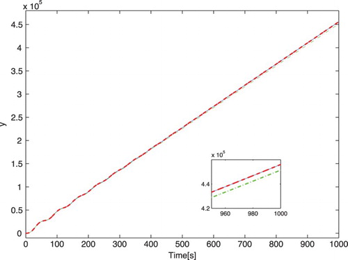
Consider first the 348th-order model of a clamped beam illustrated in Chahlaoui and Van Dooren (Citation2005). Figure shows the ramp responses of: (i) the original system, (ii) the sixth-order model retaining the original steady-state response to the ramp input, (iii) the sixth-order model obtained using Hankel-norm approximation, and (iv) the sixth-order model obtained using balanced truncation (with DC gain adjustment, thus retaining the steady-state response to a step input).
Figure 2. Ramp responses of the models of the clamped beam for the 348th-order original model (solid line) and its three sixth-order approximations obtained by the Hankel-norm model reduction (dash–dotted line), balanced truncation with DC gain adjustment (dashed line) and the proposed approach (bold dotted line). The approximation introduced by the balance truncation (with DC gain adjustment) method and by the method proposed herein are, in the considered time interval, very small and hence have not been magnified.
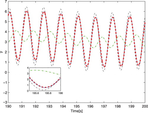
The transient component of the model that retains the steady-state component has been approximated according to the Hankel-norm criterion. Figure compares the responses to the sinusoidal input . In order to highlight the differences, attention is limited to the interval
s.
Figure 3. Responses of the models of the clamped beam to for the 348th-order original model (blue solid line), and its three sixth-order approximations obtained by the Hankel-norm model reduction (green dash–dotted line), balanced truncation with DC gain adjustment (black dashed line) and the proposed approach (red bold dashed line).
4.2. Example 2
Consider now the 48th-order model that describes the dynamics of a hospital building. This model, which is illustrated in Chahlaoui and Van Dooren (Citation2005), has also been considered in Antoulas, Sorensen, and Gugercin (Citation2001).
Figure compares again the ramp response of the original model with the ramp responses of the sixth-order models obtained by means of: (i) the proposed technique ensuring the retention of the asymptotic component, (ii) the Hankel-norm approximation, and (iii) the balanced-truncation method with DC gain adjustment. Observe, in particular, that the ramp response of the balanced-truncation model does not coincide asymptotically with the original response, as shown by the smaller picture inside the figure.
Figure 4. Ramp responses of the models of the hospital for the 48th-order original model (solid line) and its three sixth-order approximations obtained by the Hankel-norm model reduction (dash–dotted line), balanced truncation with DC gain adjustment (dashed line) and the proposed approach (bold dotted line).
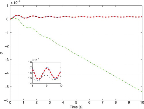
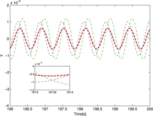
Figure compares instead the responses to the input . In this case, attention is limited to the interval
s to make the differences more visible.
Figure 5. Responses of the models of the hospital to for the 48th-order original model (blue solid line) and its three sixth-order approximations obtained by the Hankel-norm model reduction (green dash–dotted line), balanced truncation with DC gain adjustment (black dashed line) and the proposed approach (red bold dashed line).
5. Conclusions
It has been shown how standard reduction techniques can be adapted to retain the steady-state response to a numerous class of inputs, namely those expressed by a linear combination of exponentials, possibly multiplied by powers of t. This result is achieved by increasing a little the order of the reduced model with respect to the order of the models obtained from the impulse response only. This increase is negligible when the dimension of the original system is high, typically, many tens or even hundreds, as is the case in many practical applications (see, e.g. Chahlaoui and Van Dooren, Citation2005; Gawronski, Citation1998). In these cases, the resort to state-space representations is mandatory for numerical robustness. To this purpose, the components of the original forced response have preliminarily been expressed in this form.
Examples have shown that the approximation of the responses to the chosen test inputs improves significantly not only at steady state but also during the transients.
The same approach could be adopted to approximate unstable original systems by first separating the stable and unstable parts and then applying the reduction procedure to the first one only. The reduced model will finally be obtained by combining the reduced stable component with the original unstable one. In this case too, care must be taken to ensure that the reduced transfer-function denominator is the same as the denominator of the reduced stable transient term. This can again be obtained by including an auxiliary term as in (Equation12(11) ).
The approach could also be extended to the case where the input denominator has a factor in common with the denominator of the original transfer function, which would require considering a resonant or interaction term (Dorato et al., Citation1994) besides the transient and asymptotic terms.
Disclosure statement
No potential conflict of interest was reported by the authors.
References
- Antoulas, A. C. (2005). Approximation of large-scale dynamical systems. Series Advances in Design and Control, Philadelphia, PA: Society for Industrial and Applied Mathematics (SIAM).
- Antoulas, A. C., Beattie, C. A., & Gugercin, S. (2010). Interpolatory model reduction of large-scale dynamical systems. In J. Mohammadpour & K. M. Grigoriad is (Eds.), Efficient modelling and control of large-scale systems (pp. 3–58). New York, NY: Springer.
- Antoulas, A. C., Sorensen, D. C., & Gugercin, S. (2001). A survey of model reduction methods for large-scale systems (Vol. 280, pp. 193–220). Contemporary Mathematics Series. Providence, RI: American Mathematical Society.
- Astolfi, A. (2010). Model reduction by moment matching for linear and nonlinear systems. IEEE Transactions on Automatic Control, 55(10), 2321–2336. doi: 10.1109/TAC.2010.2046044
- Bernstein, D. S. (2009). Matrix mathematics: Theory, facts and formulas. Princeton, NJ: Princeton University Press.
- Bultheel, A., & De Moor, B. (2000). Rational approximation in linear systems and control. Journal of Computational and Applied Mathematics, 121(1–2), 355–378. doi: 10.1016/S0377-0427(00)00339-3
- Chahlaoui, Y., & Van Dooren, P. (2005). Benchmark examples for model reduction of linear time–invariant dynamical systems, In P. Benner, D. C. Sorensen, & V. Mehrmann (Eds.), Dimension reduction of large-scale systems (pp. 379–392). Series Lecture Notes in Computational Science and Engineering, vol. 45. Berlin: Springer.
- Chaturvedi, D. K. (2009). Modelling and simulation of systems using Matlab, Ch. 4. Boca Raton, FL: CRC Press.
- Desai, S. R., & Prasad, R. (2013). A new approach to order reduction using stability equation and big bang big crunch optimization. Systems Science & Control Engineering: An Open Access Journal, 1(1), 20–27. doi: 10.1080/21642583.2013.804463
- Dorato, P., Lepschy, A. M., & Viaro, U. (1994). Some comments on steady-state and asymptotic responses. IEEE Transactions on Education, 37(3), 264–268. doi: 10.1109/13.312135
- Gawronski, W. K. (1998). Dynamics and control of structures: A modal approach. New York, NY: Springer.
- Glover, K. (1984). All optimal Hankel-norm approximations of linear multivariable systems and their L∞ error bounds. International Journal of Control, 39(6), 1115–1193. doi: 10.1080/00207178408933239
- Kokotovic, P. V., Khail, H. K., & Reilly, J. O. (1986). Singular perturbation methods in control: Analysis and design. London: Academic Press.
- Krajewski, W., & Viaro, U. (2009). Iterative–interpolation algorithms for L2 model reduction. Control and Cybernetics, 38(2), 543–554.
- Moore, B. C. (1981). Principal component analysis in linear systems: Controllability, observability, and model reduction. IEEE Transactions on Automatic Control, 26(1), 17–32. doi: 10.1109/TAC.1981.1102568
- Ramawat, K., & Kumar, A. (2015). Improved Padé–pole clustering approach using genetic algorithm for model order reduction. International Journal of Computer Applications, 114(1), 24–28. doi: 10.5120/19943-1737
- Rana, J. S., Prasad, R., & Singh, R. (2014). Order reduction using modified pole clustering and factor division method. International Journal of Innovative Technology and Exploring Engineering, 3(11), 134–136.
- Sikander, A., & Prasad, R. 2015. Linear time invariant system reduction using mixed method approach. Applied Mathematical Modelling, doi: 10.1016/j.apm.2015.04.014, available online 23 April 2015.
- Xu, Y., & Zeng, T. (2011). Optimal H2 model reduction for large scale MIMO systems via tangential interpolation. International Journal of Numerical Analysis and Modeling, 8(1), 174–188.
- Zeng, T., & Lu, C. 2015. Two–sided Grassmann manifold algorithm for optimal H2 model reduction. International Journal of Numerical Methods in Engineering, doi: 10.1002/nme.4948, available online 14 May 2015.
Appendix
The following proposition, which is equivalent to Proposition 2.1 of Section 2, is proved next:
Proposition A.1
The forced state response of the asymptotically stable system to the causal input
(A1) with
and
is given by
(A2) with M=qI−A.
Proof.
By induction on j. To begin with, note that
and that, for any invertible matrix M,
(A3) Equation (EquationA3
(A3) ) proves the claim for j=0, in fact
which is equivalent to (EquationA2
(A2) ) for j=0. Now, suppose that (EquationA2
(A2) ) holds for a generic j. By applying the integration-by-parts rule, we obtain
(A4) By the inductive hypothesis, the third addendum in (EquationA4
(A4) ) can be written as follows:
Moreover, the fourth addendum is
which cancels the second addendum in (EquationA4
(A4) ). In addition, the first addendum can be included in the summation by simply extending it to k=−1. As a consequence,
Finally, by setting
we obtain
which proves the claim for j+1.