Experimental investigation of active yaw moment control system using a momentum wheel

ABSTRACT

Active yaw moment control is one of the most effective methods to improve the lateral stability and safety of vehicle. In this method, the overall yaw moment of the vehicle is modified by applying the corrective yaw moment generated by the systems that are mostly dependent on the tyre and road interaction. A unique technique to generate the corrective yaw moment has been considered and experimentally analysed in this work. This system utilizes a momentum wheel to generate the corrective yaw moment, which is independent of the tyre/road interaction, and is not limited by the adhesion between the tyre and road. A prototype model has been designed and developed to conduct the experimental tests and also to analyse the vehicle dynamics responses and examine the effectiveness of the designed controller. A microcontroller along with the essential sensors has been employed in the prototype to execute the embedded control system, which consists of the control algorithms, states estimator and the Kalman filter. This system provides a better vehicle performance and improves the responses of vehicle on low-friction roads. Experimental results also confirmed that the momentum wheel performance is not limited by the tyre/road adhesion condition.

KEYWORDS:

• Yaw moment control
• momentum wheel
• LQR
• Kalman filter
• estimator

Introduction

The vehicle stability and the handling performance are two important factors played in the safety of vehicle and occupants. The main objective of the vehicle stability controllers is to keep the vehicle on the desired path as close as possible (Rajamani, 2011). The yaw moment control method proved to be the most promising way to enhance the vehicle’s stability, which can be divided into three main categories of indirect, direct and integrated control as shown in Figure 1.

Figure 1. Yaw moment control aspects.

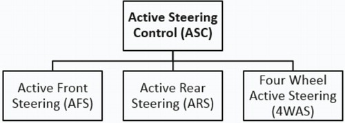
The indirect yaw moment control (DYC) method continuously modifies the vehicle steering angle in order to improve the vehicle’s total yaw moment, which is known as the active steering control (ASC) (Falcone, Borrelli, Tseng, Asgari, & Hrovat, 2008; Ikeda, 2010; Mammar & Koenig, 2002). The ASC has been implemented in vehicles in the form of an active front steering control system (Falcone, Borrelli, Asgari, Tseng, & Hrovat, 2007; Hu & He, 2011; Klier, Reimann, & Reinelt, 2004), active rear steering (Falcone et al., 2007; Hirano & Fukatani, 1997) and the four-wheel active steering (Horiuchi, Okada, & Nohtomi, 1999; Marino, Scalzi, & Cinili, 2007; Ono, Hattori, Muragishi, & Koibuchi, 2006; Yin, Chen, Wang, & Wu, 2011). All the mentioned ASC methods have shown an improvement in the vehicle handling and road stability.

The ASC system performs well in the linear region of the tyre behaviour. However, when the side-slip angle of the tyre increases beyond the saturation limits, tyres cannot produce any significant levels of lateral force, and hence, limits the performance of the ASC system into a finite region (Di Cairano & Tsengz, 2010; Nagai, Hirano, & Yamanaka, 1997).

In the DYC method, the vehicle’s yaw rate is directly controlled rather than modifying the indirect parameters, i.e. the tyres’ lateral force. Generally, the DYC can be applied by using two approaches; the first approach is to use the differential braking in which, the yaw moment is modified directly by applying the braking force onto one of the vehicle’s tyres (Boada, Boada, & Díaz, 2005; Mirzaei, 2010). The method of torque vectoring is the second approach, where the longitudinal forces on the left and right wheels are altered using the controllable final drive unit (Canale, Fagiano, Milanese, & Borodani, 2007; Osborn & Shim, 2006).

Several integrated methods (Tjonnas & Johansen, 2010; Yihu, Dandan, Zhixiang, & Xiang, 2007; Zhang, Zhang, & Zhou, 2009) have confirmed the advantages of using both the direct and indirect yaw moment control methods together to expand the system performance regions. All the yaw moment control methods discussed would depend on the road/tyre interaction. Generally, utilizing a control system that is independent of the road/tyre relation can significantly improve the control performance in the nonlinear regions of the tyre. A controlled rotating disk to control the vehicle’s yaw moment, known as the momentum wheel system has been introduced and analysed in Diba and Esmailzadeh (2012) and Goodarzi, Diba, and Esmailzadeh (2014).

In this paper, a vehicle prototype with a scaled remote controlled (RC) model car has been developed by utilizing the momentum wheel system as proposed in Diba and Esmailzadeh (2013). Several road-type tests were carried out on the developed prototype to analyse the system performance experimentally. The test results, which were analysed by using the LabVIEW software, showed that the momentum wheel system presents a superior performance to enhance the lateral dynamic of the vehicle especially on low-friction road conditions.

Vehicle model

A linear three degrees-of-freedom (DOF) vehicle model has been employed to design the control system of the momentum wheel system. The DOF of this model are the vehicle yaw rate (r), the vehicle lateral velocity (v_y) and the disk angular rate (r′). This 3-DOF vehicle model has been further developed by adding a momentum wheel at the rear-end of the well-known linear bicycle vehicle model, shown in Figure 2.

Figure 2. Linear bicycle model.

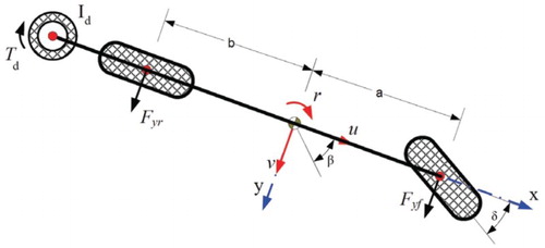
The momentum wheel system consists of a disk with its moment of inertia (I_d) and a rotary actuator. The dynamics of the rotary actuator were omitted in the system calculations. The torque (T_d) generated by the rotary actuator would be applied to the vehicle’s body in order to produce the corrective yaw moment. The vehicle’s steering angle (δ) is considered as an external disturbance. The details of the vehicle model were described in Diba and Esmailzadeh (2013).

Control structure system

The reaction torque of the momentum wheel actuator will generate the required corrective yaw moment. The linear quadratic regulator (LQR) control technique is considered to calculate the rotary actuator torque T as explained in Diba and Esmailzadeh (2013). In order to calculate the required torque, the momentum wheel controller should know the values of the steering angle, the disk angular velocity, the yaw rate and the lateral velocity of the vehicle. All these states except the last one can directly be measured. In this work, a pseudo-integral approach together with the Kalman filter has been utilized to measure the lateral and the longitudinal velocities of the vehicle.

The schematic diagram of the developed control system is shown in Figure 3. The control system comprises of mainly five major sections: the estimator, which comprises of two units of pseudo-kinematic integration and Kalman filter, the noise filter unit, the torque controller unit, and lastly, the disk controller unit. Each of these units is comprehensively described in this section.

Figure 3. Control system structure.

The vehicle states are measured using a 6-DOF inertial measurement unit (IMU module) and fed into the controller unit to calculate the actuator torque. These states are a_x, a_y and a_z, which are the longitudinal, lateral and the vertical accelerations of the vehicle, respectively. Other states are p, q and r which are the pitch, roll and the yaw rates of the vehicle, respectively. In addition to these states, there are other inputs of the control system, which are the steering angle of the vehicle δ and the momentum wheels’ angular rate r′. These two are separately measured by using two encoders.

Pseudo-kinematic integration unit

The pseudo-kinematic integration unit performs the integration process on the acceleration readings that was provided by the 6-DOF IMU module. The advantage of the pseudo-kinematic integration is to suppress the sensor noise and any drifts by blocking the integration function when it is not required, i.e. the situation in which the vehicle is completely at rest (Oh & Choi, 2012). State of the rest of vehicle is determined by using the measured data from the IMU module as shown by Equation (1) (1) where the parameter g is the acceleration due to gravity and the term represents the motion of the vehicle with its value being almost zero whenever the vehicle is at rest. This value is then compared with the user-defined threshold value and the gain of the estimator unit will then be determined as (2) The pseudo-kinematic integration unit calculates both the longitudinal velocity and the lateral velocity and then multiplies them by the estimator gain as defined in Equation (2) in order to eliminate the sensor noise during the integration process. This estimator gain is a Boolean variable, which holds the value of zero only when there is no motion.

The kinematic estimator requires the vehicle dynamics equation, which can be modelled in the state-space form as (Oh & Choi, 2012) (3) where φ is the roll angle and θ being the pitch angle. Both roll and pitch angles are directly measured by the digital motion processor in the IMU unit. The first row in Equation (3) calculates the longitudinal velocity, which can be ignored since the developed prototype would directly measure this value by the wheel sensor. Taking the two last equations into consideration, the following kinematic expression can be written as: (4) The parameters and are the respective lateral and vertical velocities estimated by the pseudo-integration method. The term v_w is the longitudinal speed of the vehicle that measured by the wheel hall sensor. Although, integration of and can lead to the drifts in the estimated velocities, but the estimate quickly returns and stabilizes to zero in order to correct the drift.

Kalman filter unit

The main application of the Kalman filter is to make the noisy measurement smooth and also produce estimate of the hidden information in the measurements. The Kalman filter can be applied to any model in which, the states of the system are continuous, observable and have a Gaussian distribution. The Kalman filter is a recursive estimator and that means to compute the estimate of the current state. The filter requires both the estimated state from the previous time step and the current measurement. Moreover, Kalman filter is able to incorporate any system modelling uncertainties and measurement noises of the sensors (Grewal & Andrews, 2011).

The Kalman filter requires the input of the measured states, z_k from the pseudo-kinematic integration unit, which contains the process noise and the measurement noise. The filter returns output of the estimated states, x_k (5) (6)

The Kalman filter uses a feedback loop to estimate the system variables and its process can be divided into two phases of the time update and the measurement update (Welch & Bishop, 1995).

Time update phase: The time update phase or predict phase would estimate the current state of the system by using the estimation of the states from the previous time step. The estimation of the predicted states is also known as the priori states estimate. The equations of this phase are accountable for projecting forward the current state and the error covariance estimates to obtain priori estimates for the next time step. Equation (7) is the predicted state estimation equation and Equation (8) represents the predicted estimate covariance (7) (8) where the matrix A is the transition matrix, which relates the state parameters at time k − 1 with the state parameters at time k. The matrix B is the control input matrix, which applies to any effect of the control input on the state vector. The matrix P is the covariance matrix and matrix Q is the process noise covariance matrix.

Measurement update phase: The measurement update phase improves the estimation of states by combining the current prediction and the current observation information. This improved estimation of the states is called posteriori states estimate. The equations of this phase are responsible for the feedback, i.e. for incorporating a new measurement into the a priori estimate to obtain an improved posteriori estimate. Equation (9) is called the innovation equation, which calculates the measurement residuals and Equation (10) represents the innovation covariance (9) (10) where is the innovation at time k which represents the error between the measured and the state estimate. The matrix H is the transformation matrix, which maps the state vector parameters into the measurement domain. The matrix S is the innovation covariance matrix and matrix R is the measurement noise covariance matrix. Equation (11) calculates the optimal gain, Equation (12) updates the estimated states and Equation (13) updates the covariance matrix (11) (12) (13) where matrix K is the Kalman gain matrix.

Noise filter unit

The noise filter unit chosen as a low-pass filter, which has been implemented in order to eliminate any jitter and the unwanted noise from the measured steering angle (δ) and the momentum wheel speed (r′).

Torque controller unit

The torque controller consists of two sections of the gain calculator and the torque calculator as shown in Figure 4. The gain calculator, which has been designed based on the LQR, computes the controller gains of the momentum wheel system as explained in Diba and Esmailzadeh (2013). These controller gains are the gain of the lateral velocity, gain of the vehicle’s yaw rate, gain of the angular speed of the momentum wheel and the gain of the steering angle, respectively.

Figure 4. Torque controller unit.

The gain calculator, which has been programmed on the microcontroller, calculates these gains every time that it receives data from the IMU unit. It can be mentioned that all these gains are function of the longitudinal velocity v_x as shown in Figure 5.

Figure 5. Controller gains vs. longitudinal velocity of vehicle. (a) Lateral velocity gain. (b) Vehicle’s yaw rate gain. (c) Disc angular velocity gain. (d) Steering angle gain.

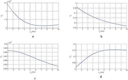
The torque calculator section will compute the required corrective yaw moment (T) by using the calculated controller gains in the form of (14)

Disk controller unit

The disk controller, which is implemented in microcontroller, will interpolate the required torque (T) into the duty cycle required to apply to the DC motor in order to achieve the torque requirements. Upon receiving the required torque signal, the disk controller performs certain calculations to determine the required velocity in order to achieve the acceleration calculated in the last step. The preceding step is to generate the respective pulse width modulation (PWM) signal by changing the duty cycle of the motor control signal. The duty cycle of the PWM wave is calculated using a conventional Proportional + Integrator (PI) controller.

Prototype development

Scaled model car

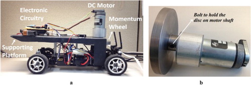
A scaled RC model car, shown in Figure 6(a), was considered to perform the experiments and also observe the vehicle dynamics behaviour. Choosing the scaled RC model car would reduce the development cost and time. Also, it provides a safe and low-cost possibility of any modification as per requirement. In the developed prototype, all the electronic circuitry, DC motor and the momentum wheel have been installed on a metallic solid platform, which has been firmly attached onto the chassis of the RC model car with the help of connecting rods. These connecting rods would also transfer the generated torque by the momentum wheel to the vehicle’s chassis. The momentum wheel has been manufactured out of a steel rod and its physical dimensions are limited by the size of the developed prototype vehicle as shown in Figure 6(b).

Figure 6. Developed RC model prototype with momentum wheel. (a) Scaled RC model car. (b) Momentum wheel (disk and DC motor).

Electrical hardware

The schematic diagram of the electirc hardware architecture is illustrated in Figure 7. The momentum wheel controller has been utilized by using the Arduino DUE microcontroller, which is a 32-bit Advanced Reduced Instruction Set Computing Machine (ARM) architechture board with a clock speed of 84 MHz (Arduino Due). The IMU module used the MPU-6050 with the on-board digital motion processor, which provides both the linear and angular accelerations of the vehicle’s chassis (MPU-6050 Accelerometer + Gyro). The steering angle module will convert the PWM signal, applied to the steering angle servo motor, into an analog signal, which is then interperated as the steering angle. The angular velocity of the wheels has been calculated by mounting the hall chip sensor on the vehicle’s wheel. The wireless transceiver transfers the measured data from the vehicle sensors to the base station by using the XBee module (XBee Wireless Transceiver). The DC motor driver will provide enough current to drive the motor and hence, generate the required torque.

Figure 7. Hardware structure diagram.

The microcontroller acquires data from all the attached sensors and then allocate the variables to different control algorithm blocks as per control design, which has been discused in section ‘Controller Structure’. After processing the data, the control algorithms would provide the end results, which are then transmitted to the base station by using the wireless transceiver module. The microcontroller board operates on a 9 V portable battery and the DC motor was powered up using the external 24 V power supply.

Experimental results and discussions

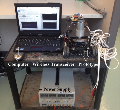
In order to analyse and evaluate the performance of the momentum wheel system, the experimental test have been conducted in a large space using the testing setup arranged as shown in Figure 8. The testing setup consists of the developed prototype, the required power supply, the wireless transceiver unit and the main computer of the system. Based on the technical limitations, a test scenario has been designed to make sure that the test conditions in every case are identical.

Figure 8. Experimental test setup with the vehicle prototype.

All the tests have been performed with a constant steering angle and over a circular path, with the fixed data update time of 25 ms. During the course of experimental tests, care has been taken to make sure that the following conditions were all been met at all time:

• Every test should start exactly from the same starting point;

• During each tests, three circular turns must have been done continuously;

• The surface condition and the vehicle tyres are the same in both tests of with and without inclusion of the momentum wheel system;

• The tolerance of the longitudinal speed (in both cases) should be within ±5% and

• The side-slip angle was calculated using the relationship .

During each tests, the vehicle yaw rate and the side-slip angle have been acquired as the measure of the handling and the safety of the vehicle, respectively. The dynamic responses of the vehicle model have been wirelessly transferred to the computer and actively analysed using the developed LabVIEW^® program, which was able to graphically demonstrate the difference between the dynamic responses of the vehicle with and without the momentum wheel system under identical conditions.

It should be mentioned that these tests were designed and performed to study the effect of the momentum wheel on the lateral dynamic of the vehicle. However, the effects of the momentum wheel on the longitudinal dynamic were not considered. Therefore, all the experimental tests were performed at a constant longitudinal velocity. The tests were performed under two different tyre/road conditions in order to observe the safety and the handling measures of the vehicle. To start every test, the prototype car has been placed at the starting point with a certain steering angle and the momentum wheel system disabled. Then it has been driven with a constant longitudinal velocity for three circular turns and their data has been collected via the LabVIEW^®. The same procedure has been repeated over again this time with the momentum wheel system engaged.

Results of low-friction road test

To decrease the friction between the prototype tyres and ground, the tyres were covered with layers of a solid lubricant. In this test, the vehicle heading angle was fixed at 25° and the longitudinal velocity was set at 2.5 m/s with the relative difference of 3%. The results of this test were illustrated in Figure 9 and the root mean square (RMS) values of the vehicle yaw rate, side-slip angle and the lateral acceleration during the test were listed in Table 1.

Figure 9. Low-friction road test results. (a) Yaw rate. (b) Side-slip angle. (c) Lateral acceleration. (d) Torque.

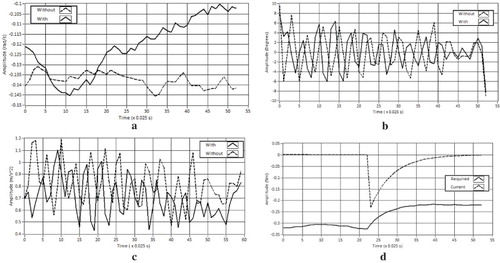
Table 1. The RMS values of the vehicle measures for low-friction road test.

Parameter	Without momentum wheel system	With momentum wheel system	Difference (%)
Yaw rate (rad/s)	−0.1218	−0.1376	+11.47
Side-slip angle (°)	3.80	3.44	−9.28
Lateral acceleration (m/s^2)	0.8239	0.7173	−12.94

It can be seen from Figure 9(a) that the vehicle with a momentum wheel system has an improved handling performance during the manoeuvre due to having a higher yaw rate. The RMS of the yaw rate for the vehicle with a momentum wheel system is almost 11.5% higher than that of the vehicle without a momentum wheel system. On the other hand, the vehicle with a momentum wheel system has enhanced its safety due to performing the manoeuvre with a lower side-slip angle and lateral acceleration, as shown in Figure 9(b) and 9(c), respectively. The RMS of the side-slip angle and the lateral acceleration of the vehicle with a momentum wheel system are almost 9.3% and 13% lower than that of the vehicle without a momentum wheel system, respectively. The required torque by the momentum wheel controller and the generated torque by the DC motor in this test are shown in Figure 9(d).

Results of high-friction road test

In this test, the vehicle’s bare tyres have been used to obtain the higher friction coefficient between the tyres and the road surface. The vehicle’s steering angle was fixed at 25° and the longitudinal speed was set at 2.15 m/s with relative difference of 4.8%. The results of this test have been illustrated in Figure 10 and the RMS measures during the test are listed in Table 2. The vehicle with a momentum wheel system has a better handling performance due to achieving a higher yaw rate during the manoeuvre, as shown in Figure 10(a). The RMS values of the yaw rate for the vehicle with a momentum wheel system is almost 6.8% higher than that of the vehicle without a momentum wheel system. As shown in Figure 10(b) and 10(c), the vehicle with a momentum wheel system has a better safety due to performing the manoeuvre with lower values of the side-slip angle and lateral acceleration. The RMS of the side-slip angle and the lateral acceleration of the vehicle with a momentum wheel system are almost 9.5% and 10% lower than that of the vehicle without a momentum wheel system, respectively. The required torque and the generated torque by the DC motor are shown in Figure 10(d).

Figure 10. High-friction road test results. (a) Yaw rate. (b) Side-slip angle. (c) Lateral acceleration. (d) Torque.

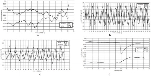
Table 2. The RMS value of the vehicle’s measures for high-friction road test.

Parameter	Without momentum wheel system	With momentum wheel system	Difference (%)
Yaw rate (rad/s)	−0.2349	−0.2199	+6.38
Side-slip angle (°)	10.87	9.83	−9.53
Lateral acceleration (m/s^2)	1.33	1.20	−10.04

Conclusions

The conventional yaw moment control methods and their strengths and weaknesses have been investigated. A new method of yaw moment control, which utilizes the momentum wheel has been studied and experimentally tested in this paper. The momentum wheel system applies the corrective yaw moment, which is independent of the tyre/road interaction. Therefore, this system would have a better dynamic performance and will enhance the vehicle dynamic responses on low-friction roads. To evaluate the performance of the momentum wheel system, a vehicle prototype has been developed using a RC car. The prototype uses a DC motor and a steel disk as the momentum wheel, which is controlled by a microcontroller installed on the prototype. The controller of the momentum wheel system has been designed by using the LQR technique. A pseudo-integration technique together with the Kalman filter has been employed to provide the best estimate of the longitudinal and lateral velocities of the vehicle. Several tests were performed using the developed prototype and their results were fully analysed. Results showed the effectiveness of the momentum wheel controller on the vehicle stability and the road handling especially on the low-friction roads. Furthermore, tests results confirmed that the performance of the momentum wheel is not limited by the tyre/road adhesion condition.

Disclosure statement

No potential conflict of interest was reported by the authors.

Additional information

Funding

The financial support provided by the Natural Science and Engineering Research Council (NSERC) of Canada to complete this research is gratefully acknowledged.

References

- Arduino Due. Retrieved June 26, 2015, from https://www.arduino.cc/en/Main/ArduinoBoardDue
- Boada, B., Boada, M., & Díaz, V. (2005). Fuzzy-logic applied to yaw moment control for vehicle stability. Vehicle System Dynamics, 43(10), 753–770. doi: 10.1080/00423110500128984
- Canale, M., Fagiano, L., Milanese, M., & Borodani, P. (2007). Robust vehicle yaw control using an active differential and IMC techniques. Control Engineering Practice, 15(8), 923–941. doi: 10.1016/j.conengprac.2006.11.012
- Diba, F., & Esmailzadeh, E. (2012, June 27–29). Dynamic performance enhancement of vehicles with controlled momentum wheel system. American Control Conference (ACC’12), Montreal, QC, pp. 6539–6544.
- Diba, F., & Esmailzadeh, E. (2013). Integrated momentum wheel and differential braking control to improve vehicle dynamic performance. Proceedings of the Institution of Mechanical Engineers, Part I: Journal of Systems and Control Engineering, 227(7), 563–576.
- Di Cairano, S., & Tsengz, H. (2010, December 15–17). Driver-assist steering by active front steering and differential braking: Design, implementation and experimental evaluation of a switched model predictive control approach. IEEE Conference on Decision and Control (CDC), Atlanta, GA, pp. 2886–2891.
- Falcone, P., Borrelli, F., Asgari, J., Tseng, H. E., & Hrovat, D. (2007). Predictive active steering control for autonomous vehicle systems. IEEE Transactions on Control Systems Technology, 15(3), 566–580. doi: 10.1109/TCST.2007.894653
- Falcone, P., Borrelli, F., Tseng, H. E., Asgari, J., & Hrovat, D. (2008). Linear time-varying model predictive control and its application to active steering systems: Stability analysis and experimental validation. International Journal of Robust and Nonlinear Control, 18(8), 862–875. doi: 10.1002/rnc.1245
- Goodarzi, A., Diba, F., & Esmailzadeh, E. (2014). Innovative active vehicle safety using integrated stabilizer pendulum and direct yaw moment control. Journal of Dynamic Systems, Measurement, and Control, 136(5), 051026-1–051026-13. doi: 10.1115/1.4027499
- Grewal, M. S., & Andrews, A. P. (2011). Kalman filtering: Theory and practice using MATLAB (4th ed.). Hoboken, NJ: John Wiley & Sons.
- Hirano, Y., & Fukatani, K. (1997). Development of robust active rear steering control for automobile. JSME International Journal Series C, 40(2), 231–238. doi: 10.1299/jsmec.40.231
- Horiuchi, S., Okada, K., & Nohtomi, S. (1999). Improvement of vehicle handling by nonlinear integrated control of four wheel steering and four wheel torque. JSAE Review, 20(4), 459–464. doi: 10.1016/S0389-4304(99)00051-X
- Hu, A., & He, F. (2011, August 8–10). Variable structure control for active front steering and direct yaw moment. 2nd International Conference on Artificial Intelligence, Management Science and Electronic Commerce (AIMSEC 2011), Deng Feng, pp. 3587–3590.
- Ikeda, Y. (2010, September 8–10). Active steering control of vehicle by sliding mode control-switching function design using SDRE. IEEE International Conference on Control Applications (CCA’10), Yokohama, pp. 1660–1665.
- Klier, W., Reimann, G., & Reinelt, W. (2004). Concept and functionality of the active front steering system (SAE Technical Paper 2004-2212).
- Mammar, S., & Koenig, D. (2002). Vehicle handling improvement by active steering. Vehicle System Dynamics, 38(3), 211–242. doi: 10.1076/vesd.38.3.211.8288
- Marino, R., Scalzi, S., & Cinili, F. (2007). Nonlinear PI front and rear steering control in four wheel steering vehicles. Vehicle System Dynamics, 45(12), 1149–1168. doi: 10.1080/00423110701214450
- Mirzaei, M. (2010). A new strategy for minimum usage of external yaw moment in vehicle dynamic control system. Transportation Research Part C: Emerging Technologies, 18(2), 213–224. doi: 10.1016/j.trc.2009.06.002
- MPU-6050 Accelerometer + Gyro. Retrieved June 26, 2015, from http://playground.arduino.cc/Main/MPU-6050
- Nagai, M., Hirano, Y., & Yamanaka, S. (1997). Integrated control of active rear wheel steering and direct yaw moment control. Vehicle System Dynamics, 27(5–6), 357–370. doi: 10.1080/00423119708969336
- Oh, J. J., & Choi, S. B. (2012). Vehicle velocity observer design using 6-D IMU and multiple-observer approach. IEEE Transactions on Intelligent Transportation Systems, 13(4), 1865–1879. doi: 10.1109/TITS.2012.2204984
- Ono, E., Hattori, Y., Muragishi, Y., & Koibuchi, K. (2006). Vehicle dynamics integrated control for four-wheel-distributed steering and four-wheel-distributed traction/braking systems. Vehicle System Dynamics, 44(2), 139–151. doi: 10.1080/00423110500385790
- Osborn, R. P., & Shim, T. (2006). Independent control of all-wheel-drive torque distribution. Vehicle System Dynamics, 44(7), 529–546. doi: 10.1080/00423110500485731
- Rajamani, R. (2011). Vehicle dynamics and control (2nd ed.). New York, NY: Springer.
- Tjonnas, J., & Johansen, T. A. (2010). Stabilization of automotive vehicles using active steering and adaptive brake control allocation. IEEE Transactions on Control Systems Technology, 18(3), 545–558. doi: 10.1109/TCST.2009.2023981
- Welch, G., & Bishop, G. (1995). An introduction to the Kalman filter (Report). Chapel Hill: University of North Carolina.
- XBee Wireless Transceiver. Retrieved June 26, 2015, from https://eewiki.net/display/Wireless/XBee+Wireless+Communication+Setup
- Yihu, W., Dandan, S., Zhixiang, H., & Xiang, Y. (2007, August 5–8). A fuzzy control method to improve vehicle yaw stability based on integrated yaw moment control and active front steering. International Conference on Mechatronics and Automation (ICMA 2007), Harbin, pp. 1508–1512.
- Yin, G.-D., Chen, N., Wang, J.-X., & Wu, L.-Y. (2011). A study on μ-synthesis control for four-wheel steering system to enhance vehicle lateral stability. Journal of Dynamic Systems, Measurement, and Control, 133(1), 011002. doi: 10.1115/1.4002707
- Zhang, S., Zhang, T., & Zhou, S. (2009, April 11–12). Vehicle stability control strategy based on active torque distribution and differential braking. International Conference on Measuring Technology and Mechatronics Automation (ICMTMA’09), Zhangjiajie, pp. 922–925.