The paradigm of complex probability and analytic linear prognostic for unburied petrochemical pipelines

ABSTRACT

Andrey Kolmogorov put forward in 1933 the five fundamental axioms of classical probability theory. The original idea in my complex probability paradigm (CPP) is to add new imaginary dimensions to the experiment real dimensions which will make the work in the complex probability set totally predictable and with a probability permanently equal to one. Therefore, adding to the real set of probabilities the contributions of the imaginary set of probabilities will make the event in absolutely deterministic. It is of great importance that stochastic systems become totally predictable since we will be perfectly knowledgeable to foretell the outcome of all random events that occur in nature. Hence, my purpose is to link my CPP to unburied petrochemical pipelines’ analytic prognostic in the linear damage accumulation case. Consequently, by calculating the parameters of the novel prognostic model, we will be able to determine the magnitude of the chaotic factor, the degree of knowledge, the complex probability, the system failure and survival probabilities, and the remaining useful lifetime probability, after a pressure time t has been applied to the pipeline, and which are all functions of the system degradation subject to random effects.

KEYWORDS:

• Complex set
• probability norm
• degree of our knowledge
• chaotic factor
• linear damage
• degradation
• remaining useful lifetime
• analytic prognostic

Nomenclature

	=	real probability set of events
	=	imaginary probability set of events
	=	complex probability set of events
i	=	the imaginary number where
EKA	=	extended Kolmogorov's axioms
CPP	=	complex probability paradigm
Prob	=	probability of any event
Pr	=	probability in the real set  = system failure probability
Pm	=	probability in the imaginary set corresponding to the real probability in  = system survival probability in
Pm/i	=	system survival probability in
Pc	=	probability of an event in with its associated event in , it is the probability in the complex set
Z	=	complex probability number and vector, it is the sum of Pr and Pm
DOK =	=	degree of our knowledge of the random experiment and event, it is the square of the norm of Z
Chf	=	Chaotic factor
MChf	=	magnitude of the chaotic factor
t	=	pressure cycles time
tC	=	pressure cycles time till system failure
	=	pipelines’ internal triangular pressure
fj(t)	=	probability density function for each pressure mode j
F(t)	=	cumulative distribution function
	=	simulation magnifying factor for each pressure mode j
D	=	degradation indicator of a system
RUL	=	remaining useful lifetime of a system
Prob[RUL(t)]	=	probability of RUL after a pressure cycles time t

I. Introduction

Firstly, in this introductory section an overview of the history of probability theory will be done. Etymologically, probable and probability and their cognates in other modern languages derive from mediaeval-learned Latin probabilis and deriving from Cicero and generally applied to an opinion to mean plausible or generally approved (Franklin, 2001). The mathematical sense of the term is from 1718. The term chance was also used in the eighteenth century in the mathematical sense of ‘probability’ and probability theory was called Doctrine of Chances. This word is ultimately from Latin cadentia; that is, ‘a fall case’. The English adjective likely is of Germanic origin, most likely from Old Norse likligr, knowing that Old English had geliclic with the same sense, and originally meaning ‘having the appearance of being strong or able’ and ‘having the similar appearance or qualities’, with a meaning of ‘probably’ recorded from the late fourteenth century. Similarly, the derived noun likelihood had a meaning of ‘similarity, resemblance’ but took on a meaning of ‘probability’ from the mid-fifteenth century (Freund, 1973; Kuhn, 1970; Warusfel & Ducrocq, 2004; Wikipedia, the free encyclopedia, Probability; Wikipedia, the free encyclopedia, Probability Distribution; Wikipedia, the free encyclopedia, Probability Theory).

Moreover, probability has a dual aspect: on the one hand, the likelihood of hypotheses given the evidence for them, and on the other hand, the behaviour of stochastic processes such as the throwing of dice or coins. The study of the former is historically older in, for example, the law of evidence, while the mathematical treatment of dice began with the work of Gerolamo Cardano, Blaise Pascal, and Pierre de Fermat, between the sixteenth and seventeenth centuries. Knowing that, probability is distinguished from statistics. In fact, while statistics deals with data and inferences from it, probability deals with the stochastic or random processes which lie behind data or outcomes (Abrams, 2008; Daston, 1988; Hacking, 2006; Jeffrey, 1992; Poincaré, 1968; Stewart, 1996, 2012).

Furthermore, ancient and mediaeval law of evidence developed a grading of degrees of proof, probabilities, presumptions, and half-proof, to deal with the uncertainties of evidence in court (Franklin, 2001). In Renaissance times, betting was discussed in terms of odds such as ‘ten to one’ and maritime insurance premiums were estimated based on intuitive risks, but there was no theory on how to calculate such odds or premiums (Franklin, 2001). The mathematical methods of probability arose in the year 1654 in the correspondence of Cardano, Fermat and Pascal on such questions as the fair division of the stake in an interrupted game of chance. In the year 1657, Christiaan Huygens gave a comprehensive treatment of the subject (Franklin, 2001; Hacking, 2006).

Also, from the book Games, Gods and Gambling by David (1962), we will quote:

In ancient times there were games played using astragali, or Talus bone. The Pottery of ancient Greece was evidence to show that there was a circle drawn on the floor and the astragali were tossed into this circle, much like playing marbles. In Egypt, excavators of tombs found a game they called ‘Hounds and Jackals’ which closely resembles the modern game ‘Snakes and Ladders’. It seems that this is the early stages of the creation of dice. The first dice game mentioned in literature of the Christian era was called Hazard. Played with 2 or 3 dice. Thought to have been brought to Europe by the knights returning from the Crusades. Dante Alighieri (1265–1321) mentions this game. A commenter of Dante puts further thought into this game: the thought was that with 3 dice, the lowest number you can get is 3, an ace for every die. Achieving a 4 can be done with 3 die by having a two on one die and aces on the other two dice. Cardano also thought about the throwing of three die. 3 dice are thrown: there are the same number of ways to throw a 9 as there are a 10. For a 9: (621) (531) (522) (441) (432) (333) and for 10: (631) (622) (541) (532) (442) (433). From this, Cardano found that the probability of throwing a 9 is less than that of throwing a 10. He also demonstrated the efficacy of defining odds as the ratio of favourable to unfavourable outcomes (which implies that the probability of an event is given by the ratio of favourable outcomes to the total number of possible outcomes Gorrochum, 2012; Von Plato, 1994). In addition, the famous Galileo Galilei wrote about die-throwing sometime between 1613 and 1623. Essentially thought about Cardano’s problem, about the probability of throwing a 9 is less than throwing a 10. Galileo had the following to say: Certain numbers have the ability to be thrown because there are more ways to create that number. Although 9 and 10 have the same number of ways to be created, 10 is considered by dice players to be more common than 9.

Additionally, Jacob Bernoulli's Ars Conjectandi (posthumously in 1713) and Abraham de Moivre's The Doctrine of Chances (in 1718) put probability on a sound mathematical footing, showing how to calculate a wide range of complex probabilities. Bernoulli proved a version of the fundamental law of large numbers, which states that in a large number of trials, the average of the outcomes is likely to be very close to the expected value – for example, in 1000 throws of a fair coin, it is likely that there are close to 500 heads, and the larger the number of throws, the closer to half-and-half the proportion is likely to be (Barrow, 1992; Bogdanov & Bogdanov, 2009, 2010, 2012, 2013; Greene, 2003; Hawking, 2005; Penrose, 1999).

Moreover, the power of probabilistic methods in dealing with uncertainty was shown by Carl Friedrich Gauss's (the prince of mathematicians) determination of the orbit of the asteroid Ceres from a few observations. The theory of errors used the method of least squares to correct error-prone observations, especially in astronomy, based on the assumption of a normal distribution of errors to determine the most likely true value. In 1812, Marquis Pierre-Simon de Laplace issued his Théorie analytique des probabilités in which he consolidated and laid down many fundamental results in probability and statistics such as the moment generating function, method of least squares, inductive probability, and hypothesis testing. Towards the end of the nineteenth century, a major success of explanation in terms of probabilities was the Statistical mechanics of Ludwig Boltzmann and Josiah Willard Gibbs which explained properties of gases such as temperature in terms of the random motions of large numbers of particles. Knowing that, the field of the history of probability itself was established by Isaac Todhunter's monumental A History of the Mathematical Theory of Probability from the Time of Pascal to that of Laplace which was published in 1865 (Aczel, 2000; Boltzmann, 1995; Cercignani, 2010; Davies, 1993; Hawking, 2002, 2011; Reeves, 1988; Ronan, 1988; Seneta, 2016; Pickover, 2008; Planck, 1969).

In addition, probability and statistics became closely connected through the work on hypothesis testing of Ronald Aylmer Fisher and Jerzy Neyman, which is now widely applied in biological and psychological experiments and in clinical trials of drugs, as well as in economics and elsewhere. A hypothesis, for example, that a drug is usually effective gives rise to a probability distribution that would be observed if the hypothesis is true. If observations approximately agree with the hypothesis, it is confirmed, if not, the hypothesis is rejected (Hald, 1998, 2003; Heyde & Seneta, 2001; Mcgrayne, 2011; Salsburg, 2001; Stigler, 1990). Furthermore, the theory of stochastic processes broadened into such areas as Markov processes (named after the Russian mathematician Andrey Markov) and Brownian motion (named after the Scottish botanist Robert Brown) which is the random movement of tiny particles suspended in a fluid. That provided a model for the study of random fluctuations in stock markets, leading to the use of sophisticated probability models in mathematical finance, including such successes as the widely used Black–Scholes formula developed by Fischer Black and Myron Scholes in their 1973 paper for the valuation of options (Bernstein, 1996; Ivancevic & Ivancevic, 2008; http://www.statslab.cam.ac.uk/∼rrw1/markov/M.pdf). Also, the twentieth century saw long-running disputes on the interpretations of probability. In the mid-century ‘frequentism’ was dominant, holding that probability means long-run relative frequency in a large number of trials. At the end of the century there was some revival of the Bayesian view, according to which the fundamental notion of probability is how well a proposition is supported by the evidence for it. The mathematical treatment of probabilities, especially when there are infinitely many possible outcomes, was facilitated by Andrey Nikolaevich Kolmogorov's axioms in 1933 (Balibar, 2002; Burgi, 2010; Hoffmann, 1975; Moore, 1992; Vitanyi, 1988).

Secondly, also in this section, prognostic theory in addition to my adopted model will be introduced. The high availability of technological systems like aerospace, defence, petro-chemistry, and automobile industries is an important major goal of earlier recent developments in system design technology. In petrochemical industries, pipelines are the principal element of hydrocarbon transport systems. They are crucial for human activities since they serve to transport oil, water, and natural gases from sources to all sites of consumers. A new analytic prognostic model was developed in my previous papers and applied to the case of pipes subject to internal pressure, to the effects of corrosion, and to soil loading. This will initiate micro-cracks in the tube’s body that can propagate suddenly and can lead to failure. The increase of pipes’ performance, availability, and the reduction of their global mission cost need to be investigated using a suitable prognostic process. Consequently, a new approach based on analytic laws of degradation was applied to different dynamic systems and was proposed in my research papers (Abou Jaoude, 2015a; Abou Jaoude & El-Tawil, 2013a; Abou Jaoude, El-Tawil, Kadry, Noura, & Ouladsine, 2010; Abou Jaoude, Kadry, El-Tawil, Noura, & Ouladsine, 2011; El-Tawil, Kadry, & Abou Jaoude, 2009; El-Tawil, Abou Jaoude, Kadry, Noura, & Ouladsine, 2010). Furthermore, from a predefined threshold of degradation, the remaining useful lifetime (RUL) was estimated. Based on a physical petrochemical pipeline system, my research work elaborated a procedure to create a failure prognostic model that will be more developed and further improved in the current paper.

Furthermore, prognostic is a process encompassing a capacity of prediction. It is the ability to estimate the RUL of equipment in terms of its functioning history and its future usage. Predicting the RUL of industrial systems becomes currently an important aim for industrialists knowing that the failure, whose consequences are generally very expensive, can occur suddenly. The classical strategies of maintenance (Lemaitre & Chaboche, 1990; Vachtsevanos, Lewis, Roemer, Hess, & Wu, 2006) based on a static threshold of alarm are no more efficient and practical because they do not take into consideration the instantaneous product functioning state. The introduction of a prognostic approach as an ‘intelligent’ maintenance consists of the analysis, the health follow-up, and monitoring, based on physical measurements using sensors.

Moreover, previous specialized prognostic studies belong generally to three types of models: the first type is the ‘experience-based models’ (Vasile, 2008) (based on measurements taken from health monitoring of machines like for example those based on expert judgement, stochastic model, Markovian process, Bayesian approach, Reliability analysis, Optimization of preventive maintenance, etc.). Their prognostic methodology proves to be simple but inflexible towards changes in system behaviour and environment. The second type is the ‘data-based models’ relying on the statistics of large measured data (as examples we can cite the work based on degradation behaviour described by abaci and using an expert description of the system: Process–Mission–Environment (Peysson et al., 2009), the work based on artificial intelligence, machine learning (Proteus WP2 Team, 2005); neural network (Vasile, 2008); fuzzy logic (Concha, 2007), etc.). Their methodologies are described as not very precise and efficient. The third type is the ‘Physical models’ based on mathematical description of the degradation process and its level evolution using NDI monitoring (Non-Destructive Inspection). It is described to be more flexible and precise than the two first types (Figure 1). My previous work presents an analytical prognostic methodology based on analytic laws of damage, such as Paris-Erdogan's law of fatigue crack propagation and Palmgren–Miner's law of linear damage accumulation. It belongs to the third type of models. Whenever the damage law of the studied system is available analytically, the advantage of this approach is its realistic and precise features in determining the system RUL (Abou Jaoude, 2012; Abou Jaoude, El-Tawil, Kadry, Noura, & Ouladsine, 2011; Abou Jaoude, Noura, El-Tawil, Kadry, & Ouladsine, 2012a, 2012b).

Figure 1. The prognostic approaches.

Additionally, pipelines are petrochemical systems transporting oil and natural gas over long distances and in huge quantities. Their life prognostic is vital in this industry since their availability has crucial consequences. Their main failures are due to seismic ground waves, soil settlements, buckling, deformations, internal and external corrosion, stress concentration in welding and fitting, vibration and resonance, and pressure fluctuation over a long period. The fatigue failures by crack propagation are detected by crack detection tools. Hence, three case studies of pipes were considered in my previous research work (Abou Jaoude, 2013a; Abou Jaoude & El-Tawil, 2013b; El-Tawil & Abou Jaoude, 2013): unburied, buried, and subsea (offshore pipes). Each one of these situations requires different physical parameters such as corrosion, soil pressure, and friction, and water and atmospheric pressure. The unburied pipes case will only be considered in the current paper.

Thirdly and finally, to conclude, this research paper is organized as follows: After the introduction in Section 1, the purpose and the advantages of the present work are presented in Section 2. Afterwards, in Section 3, the complex probability paradigm (CPP) with its original parameters and interpretation will be explained and illustrated. In Section 4, my published analytic prognostic model of fatigue for unburied pipeline systems in the linear cumulative damage case is recapitulated. Furthermore, in Section 5, the CPP’s new and basic assumptions are laid down, elaborated, and applied to analytic linear prognostic. Furthermore, the simulations of the novel model for the three pressure conditions and modes are illustrated in Section 6. Finally, we conclude the work by presenting a comprehensive summary in Section 7, and then present the list of references cited in the current research work.

2. The purpose and the advantages of the present work

All our work in classical probability theory is to compute probabilities. The original idea in this paper is to add new dimensions to our random experiment which will make the work totally deterministic. In fact, probability theory is a nondeterministic theory by nature; that means that the outcome of the stochastic events is due to chance and luck. By adding new dimensions to the event occurring in the ‘real’ laboratory which is , we make the work deterministic and hence a random experiment will have a certain outcome in the complex set of probabilities . It is of great importance that stochastic systems become totally predictable since we will be perfectly knowledgeable to foretell the outcome of all chaotic and random events that occur in nature like for example in statistical mechanics, in all stochastic processes, or in the well-established field of prognostic. Therefore, the work that should be done is to add to the real set of probabilities the contributions of which is the imaginary set of probabilities that will make the event in absolutely deterministic. If this is found to be fruitful, then a new theory in stochastic sciences and prognostic would be elaborated and this to understand deterministically those phenomena that used to be random phenomena in . This is what I called ‘The CPP’ that was initiated and elaborated in my eight previous papers (Abou Jaoude, 2013b, 2013c, 2014, 2015b, 2015c, 2016a, 2016b; Abou Jaoude, El-Tawil, & Kadry, 2010).

Moreover, although the analytic linear prognostic laws are deterministic and very well presented in Abou Jaoude et al. (2012a) there are random and chaotic factors (such as temperature, humidity, geometry dimensions, material nature, water action, applied load location, atmospheric pressure, corrosion, soil pressure, and friction) that affect the unburied pipeline system and make its degradation function deviate from its calculated trajectory predefined by these deterministic laws. An updated follow-up of the degradation behaviour with time or cycle number, and which is subject to chaotic and non-chaotic effects, is done by what I called the system failure probability due to its definition that evaluates the jumps in the degradation function D.

Furthermore, my purpose in this current work is to link the CPP to the unburied pipeline system analytic prognostic in the linear damage accumulation case and which is subject to fatigue. In fact, the system failure probability derived from prognostic will be included in and applied to the CPP. This will lead to the novel and original prognostic model illustrated in this paper. Hence, by calculating the parameters of the new prognostic model, we will be able to determine the magnitude of the chaotic factor, the degree of our knowledge (DOK), the complex probability, the system failure and survival probabilities, and the RUL probability; after that a pressure cycles time t has been applied to the unburied pipeline, which are all functions of the system degradation subject to chaos and random effects.

Consequently, to summarize, the objectives and the advantages of the present work are to:

1. Extend classical probability theory to the set of complex numbers, and hence to relate probability theory to the field of complex analysis in mathematics. This task was initiated and elaborated in my eight previous papers.

2. Do an updated follow-up of the degradation D behaviour with time or cycle number which is subject to chaos. This follow-up is accomplished by the system real failure probability due to its definition that evaluates the jumps in D; and hence to relate probability theory to a system degradation in an original and a new way.

3. Apply the new probability axioms and paradigm to prognostic; thus, I will extend the concepts of prognostic to the complex probability set .

4. Prove that any random and stochastic phenomenon can be expressed deterministically in the complex set .

5. Quantify both the DOK and the chaos magnitude of the system degradation and its RUL.

6. Draw and represent graphically the functions and parameters of the novel paradigm associated with an unburied pipeline prognostic.

7. Show that the classical concepts of random degradation and RUL have a probability of occurring always equal to 1 in the complex set; hence, no chaos, no disorder, and no ignorance exist in (complex set) =  (real set) +  (imaginary set).

8. Prove that by adding supplementary and new dimensions to any random experiment whether it is a pipeline system or any other stochastic system we will be able to do prognostic in a deterministic way in the complex set .

9. Pave the way to apply the original paradigm to other topics in statistical mechanics, in stochastic processes, and to the field of prognostics in engineering and science. These will be the subjects of my subsequent research papers.

Concerning some applications of the novel proposed prognostic paradigm and as a future work, it will be applied to a wide set of dynamic systems like vehicle suspension systems and buried and offshore petrochemical pipelines which are subject to fatigue and in the linear and nonlinear damage accumulation cases.

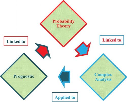
To conclude, compared with existing literature, the main contribution of the current research paper is to apply the original CPP to the concepts of random degradation and RUL of an unburied pipeline system and thus to the field of analytic prognostic in the linear damage accumulation case subject to fatigue.

Figure 2 summarizes the objectives of the current research paper.

Figure 2. The diagram of the principal objectives of this research work.

3. The extended set of probability axioms

In this section, the extended set of probability axioms of the CPP will be presented.

3.1. The original Andrey Nikolaevich Kolmogorov set of axioms

The simplicity of Kolmogorov's system of axioms may be surprising. Let E be a collection of elements {E₁, E₂, … } called elementary events and let F be a set of subsets of E called random events. The five axioms for a finite set E are (Benton, 1966a, 1966b; Feller, 1968; Montgomery & Runger, 2003; Walpole, Myers, Myers, & Ye, 2002):

• Axiom 1: F is a field of sets.

• Axiom 2: F contains the set E.

• Axiom 3: A non-negative real number P_rob(A), called the probability of A, is assigned to each set A in F. We have always 0 ≤ P_rob(A) ≤ 1.

• Axiom 4: P_rob(E) equals 1.

• Axiom 5: If A and B have no elements in common, the number assigned to their union is:

• hence, we say that A and B are disjoint; otherwise, we have

And we say also that which is the conditional probability. If both A and B are independent then: .

Moreover, we can generalize and say that for N disjoint (mutually exclusive) events (for ), we have the following additivity rule: And we say also that for N independent events (for ), we have the following product rule:

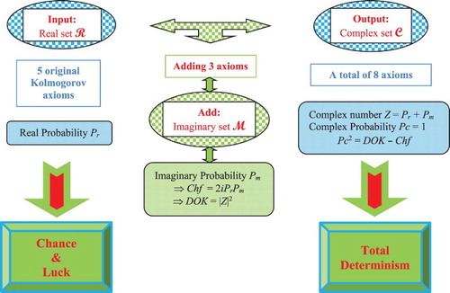
3.2. Adding the imaginary part

Now, we can add to this system of axioms an imaginary part such that

• Axiom 6: Let be the probability of an associated event in (the imaginary part) to the event A in (the real part). It follows that , where i is the imaginary number with .

• Axiom 7: We construct the complex number or vector having a norm such that: .

• Axiom 8: Let Pc denote the probability of an event in the complex probability universe where . We say that Pc is the probability of an event A in with its associated event in such that:

• and is always equal to 1.

We can see that the system of axioms defined by Kolmogorov could be hence expanded to take into consideration the set of imaginary probabilities by adding three new axioms (Abou Jaoude, 2013b, 2013c, 2014, 2015b, 2015c, 2016a, 2016b; Abou Jaoude et al., 2010).

3.3. The purpose of extending the axioms

It is apparent from the set of axioms that the addition of an imaginary part to the real event makes the probability of the event in always equal to 1. In fact, if we begin to see the set of probabilities as divided into two parts, one is real and the other is imaginary, understanding will follow directly. The random event that occurs in the real probability set (like tossing a coin and getting a head), has a corresponding probability . Now, let be the set of imaginary probabilities and let be the DOK of this phenomenon. is always, and according to Kolmogorov's axioms, the probability of an event.

A total ignorance of the set makes:

and in this case is equal to: Conversely, a total knowledge of the set in makes:

and P_m = P_rob(imaginary part) = 0. Here we have because the phenomenon is totally known, that is, its laws and variables are completely determined, hence; our DOK of the system is 1 = 100%.

Now, if we can tell for sure that an event will never occur, i.e. like ‘getting nothing’ (the empty set), is accordingly = 0, that is the event will never occur in . will be equal to:

, and , because we can tell that the event of getting nothing surely will never occur; thus, the DOK of the system is 1 = 100%. (Abou Jaoude et al., 2010)

We can infer that we have always: (1) And what is important is that in all cases, we have (2) In fact, according to an experimenter in , the game is a game of chance: the experimenter does not know the output of the event. He will assign to each outcome a probability and he will say that the output is nondeterministic. But in the universe , an observer will be able to predict the outcome of the game of chance since he takes into consideration the contribution of , so we write:

Hence, is always equal to 1. In fact, the addition of the imaginary set to our random experiment resulted in the abolition of ignorance and indeterminism. Consequently, the study of this class of phenomena in is of great usefulness since we will be able to predict with certainty the outcome of experiments conducted. In fact, the study in leads to unpredictability and uncertainty. So instead of placing ourselves in , we place ourselves in then study the phenomena, because in the contributions of are taken into consideration and therefore a deterministic study of the phenomena becomes possible. Conversely, by taking into consideration the contribution of the set we place ourselves in and by ignoring we restrict our study to nondeterministic phenomena in (Bell, 1992; Boursin, 1986; Dacunha-Castelle, 1996; Srinivasan and Mehata 1988; Stewart, 2002; Van Kampen, 2006).

Moreover, it follows from the above definitions and axioms that (Abou Jaoude et al., 2010): (3) will be called the Chaotic factor in our experiment and will be denoted accordingly by ‘Chf’. We will see why we have called this term the chaotic factor; in fact:

In case , that is the case of a certain event, then the chaotic factor of the event is equal to 0.

In case , that is the case of an impossible event, then Chf = 0. Hence, in both the two last cases, there is no chaos since the outcome is certain and is known in advance.

In case , . (Figures 3–5)

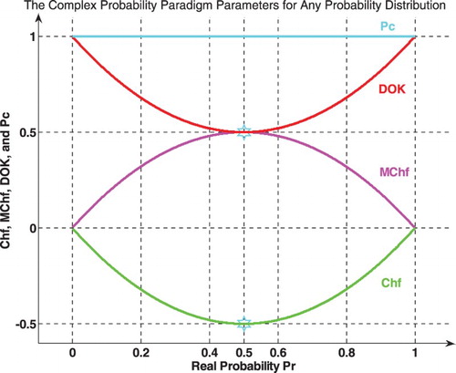
Figure 3. Chf, DOK, and Pc for any probability distribution in 2D.

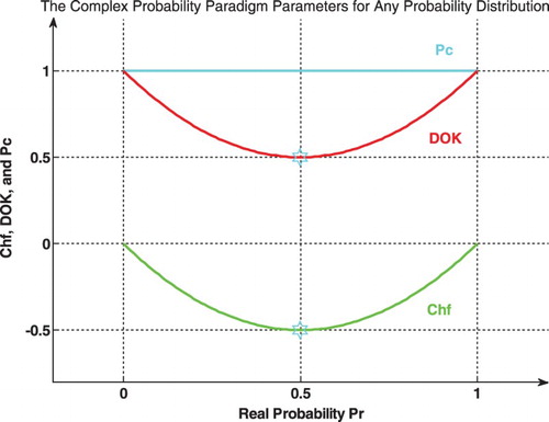
Figure 4. DOK, Chf, and Pc for any probability distribution in 3D with .

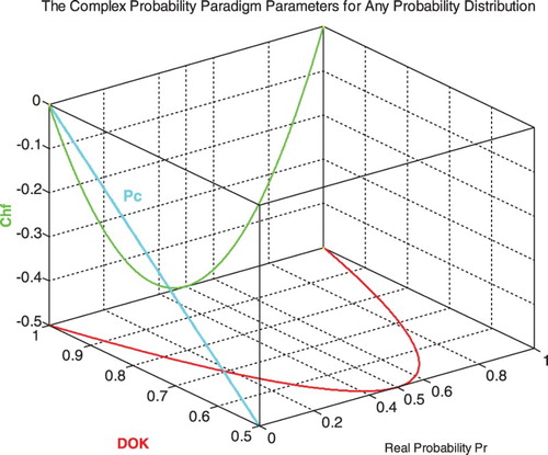
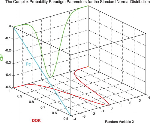
Figure 5. DOK, Chf, and Pc for the standard normal probability distribution in 3D with .

We notice that: .

What is interesting here is thus we have quantified both the DOK and the chaotic factor of any random event and hence we write now: (4) Then we can conclude that: therefore permanently.

This directly means that if we succeed to subtract and eliminate the chaotic factor in any random experiment, then the output will always be with a probability equal to 1 (Dalmedico-Dahan & Peiffer, 1986; Dalmedico-Dahan, Chabert, & Chemla, 1992; Ekeland, 1991; Gleick, 1997; Gullberg, 1997; Science et Vie, 1999).

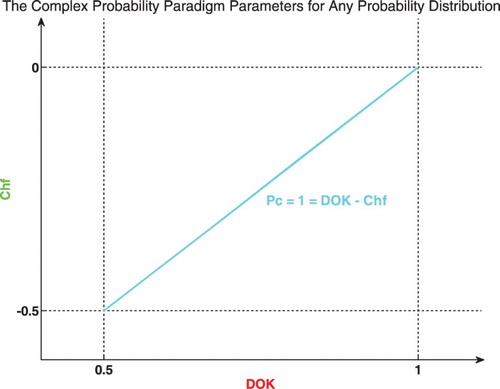
The graph below shows the linear relation between both DOK and Chf (Figure 6).

Figure 6. Graph of for any probability distribution.

Furthermore, we need in our current study the absolute value of the chaotic factor that will give us the magnitude of the chaotic and random effects on the studied system materialized by the random pressure cycles time t and a probability density function (PDF), and which lead to an increasing system chaos in and sometimes to a premature system failure. This new term will be denoted accordingly MChf or Magnitude of the Chaotic factor (Abou Jaoude, 2015b, 2015c, 2016a, 2016b). Hence, we can deduce the following: (5) And where .

The graph (Figure 7) shows the linear relation between both DOK and MChf. Moreover, Figures 8–14 show the graphs of Chf, MChf, DOK, and Pc as functions of the real probability P_r for any probability distribution and for a standard normal distribution.

Figure 7. Graph of for any probability distribution.

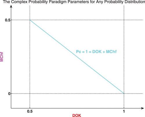
Figure 8. MChf, DOK, and Pc for any probability distribution in 2D.

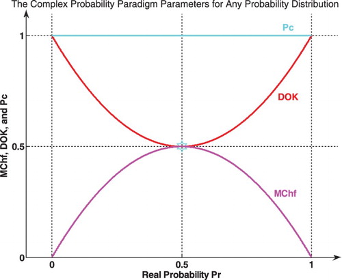
Figure 9. DOK, MChf, and Pc for any probability distribution in 3D with .

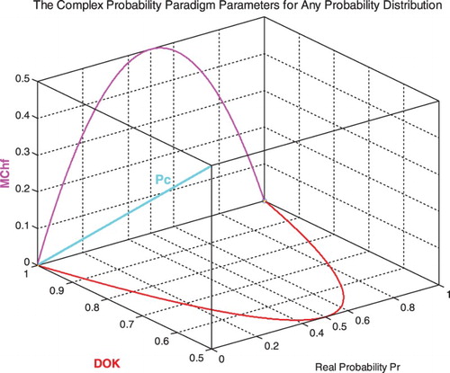
Figure 10. DOK, MChf, and Pc for the standard normal probability distribution in 3D with .

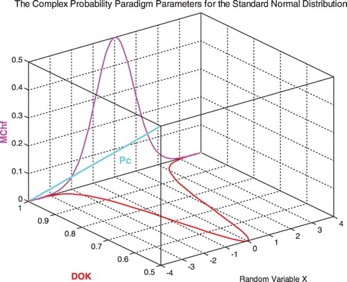
Figure 11. Chf and MChf for any probability distribution in 2D.

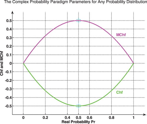
Figure 12. Chf and MChf for any probability distribution in 3D with MChf + Chf = 0.

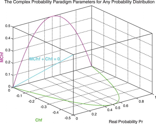
Figure 13. Chf and MChf for the standard normal probability distribution in 3D with MChf + Chf = 0.

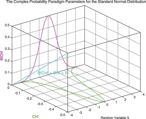
Figure 14. Chf, MChf, DOK, and Pc for any probability distribution in 2D.

To summarize and to conclude, as the degree of our certain knowledge in the real universe is unfortunately incomplete, the extension to the complex set includes the contributions of both the real set of probabilities and the imaginary set of probabilities . Consequently, this will result in a complete and perfect degree of knowledge in (since Pc = 1). In fact, in order to have a certain prediction of any random event, it is necessary to work in the complex set in which the chaotic factor is quantified and subtracted from the computed degree of knowledge to lead to a probability in equal to one (Pc²  = DOK − Chf = DOK + MChf = 1). This hypothesis is verified in my eight previous research papers by the mean of many examples encompassing both discrete and continuous distributions (Abou Jaoude, 2013b, 2013c, 2014, 2015b, 2015c, 2016a, 2016b; Abou Jaoude et al., 2010). The Extended Kolmogorov Axioms (EKA for short) or the CPP can be illustrated by Figure 15:

Figure 15. The EKA or the CPP diagram.

4. Previous research work: analytic prognostic and linear damage accumulation

In this section a comprehensive summary of a part of my previously published Ph.D. thesis (Abou Jaoude, 2012) and of the formerly published IFAC conference paper (Abou Jaoude et al., 2012a) will be presented and the results that this current article needs will be just cited.

4.1. A brief introduction to the adopted methodology (Abou Jaoude, 2012; Abou Jaoude et al., 2012a)

The purpose of my previous research work, which will be improved in the current paper and will be related to CPP, was to create an analytic linear model of prognostic capable of predicting the degradation D and the RUL trajectories of an unburied petrochemical pipeline system subject to fatigue under a given environment and starting from an initial known damage.

Pipelines are petrochemical systems that serve to transport oil and natural gas between sites. Pipelines’ tubes are considered as a principal component in petrochemical industries, their life prognostic is vital in this industry since their availability has crucial consequences for the exploitation cost. The main failure cause for these systems is the fatigue due to internal pressure-depression variation along the time.

These pipelines are usually designed for ultimate limits states (resistance). Moreover, buried pipelines are subject to corrosion due to soil aggression effects. Pipelines are manufactured as cylindrical tubes of radius R and of thickness e.

The DNV 2000 rules propose for pipelines a target probability of failure about 10⁻⁵. Their main failures are due to seismic ground waves, soil settlements, buckling, deformations, internal and external corrosion, stress concentration in welding and fitting, vibration and resonance, and pressure fluctuation over a long period. In addition, the fatigue failures by crack propagation are detected by crack detection tools.

A significant part of main pipelines are subjected to external cracking, which is a serious problem for the pipeline industry like, for example, in Russia, the U.S.A., and Canada. Identification of external cracks is achieved using different Nondestructive Evaluation methods. If cracks are revealed during inspection, their influence on the RUL of the pipeline should be assessed in order to choose what maintenance action should be used: do nothing/repair/replace. Pipeline integrity is assessed on the assumption that some defects after In-Line Inspection may be: still undetected; detected, but not measured; detected and measured.

Furthermore, the aim in my research work was to evaluate the evolution of the system lifetime at each instant. For this purpose the degradation trajectories had been used in terms of cycles' numbers or the time of operation. From these degradation trajectories, the RULs variations were deduced. Therefore, to demonstrate the effectiveness of my model, many industrial examples had been considered in the model simulation in these previous research papers and work (Abou Jaoude, 2012, 2013a, 2015a; Abou Jaoude & El-Tawil, 2013a, 2013b; Abou Jaoude, El-Tawil et al., 2011; Abou Jaoude, El-Tawil, Kadry, Noura, & Ouladsine, 2010; Abou Jaoude, Kadry et al., 2011; Abou Jaoude et al., 2012a, 2012b; El-Tawil et al., 2009, 2010; El-Tawil & Abou Jaoude, 2013). Three case studies of pipes were considered: unburied, buried, and subsea (offshore pipes). Each one of these situations requires different physical parameters such as corrosion, soil pressure and friction, and water and atmospheric pressure. One of these examples is discussed here which is the unburied petrochemical pipeline system where three modes of pressure profiles (high = mode 1, middle = mode 2, and low-pressure conditions = mode 3) were simulated and examined. In such industrial systems, my model proved that it is very convenient and it provided a useful tool for a prognostic analysis. Additionally, it is less expensive than other models that need a large number of data and measurements.

4.2. Fatigue crack growth

The stress intensity factor was introduced for the correlation between the crack growth rate, da/dN, and the stress intensity factor range, ΔK. Paris-Erdogan's law (Lemaitre & Chaboche, 1990) permits to determine the propagation rate of the crack length a after its detection. This law of damage growth is given by the equation: (6) where  =the increase of the crack length a per cycle N=crack growth rate. =the stress intensity factor.  = the function of the component's crack geometry.  = the range of the applied stress in a cycle. C and m = experimentally obtained constants of materials; and .

4.3. The linear cumulative damage modelling

To study the prognosis of a degrading component, my idea is to predict and estimate the end of life of the component by tracking and modelling the degradation function. My damage model whose evolution is up to the point of macro-crack initiation is represented in Figure 16 by Palmgren-Miner's linear rule of damage. In fact, this law (Lemaitre & Chaboche, 1990) serves to compute the cumulative damage d_i of different stresses levels σ_i (i = 1, i = 2, … , i = k) applied for n_i cycles. Knowing that, N_i is the total cycle's number of stress σ_i to be applied and that leads to failure. The linear cumulative damage relative to the applied stresses (i = 1 to k) is given by (7) To facilitate the analysis, it is convenient to adopt a damage measurement evaluated by the linear cumulative damage law of Palmgren–Miner. The state of damage in a specimen at a particular cycle during fatigue is represented by a scalar damage function D(N). The value D = 0 corresponds to no damage, and D = 1 corresponds to the appearance of the first macro-crack (total damage).

Figure 16. Palmgren-Miner's linear rule of damage.

4.4. An expression for degradation

The initial detectable crack at the cycle N₀, the crack length at any cycle N, and the crack length at the failure cycle N_C are measured by a sensor and their values are incorporated in the damage prognostic model through the damage equation. It is given in my model by the following expression: (8) Therefore, my general prognostic analytic linear model function, which is a recursive relation for the sequence of D, is given by Abou Jaoude (2012): (9) where C is the environment parameter, e is the pipe thickness, R is the pipe radius, is the initial crack length at the cycle N₀, is the crack length at the load cycle N − 1, and is the crack length at the failure cycle N_C. It was assumed in the model that for justified reasons (Abou Jaoude, 2012), is the pipe internal pressure.

Consequently, the previous recursive relation leads to a sequence of D_N values with or and whose limit is D_C = 1: (10) To take into account various states of pressure conditions, three different types of internal pressure will be considered, which are high, middle, and low. Furthermore, as the stress-load is expressed in terms of time t or N, then we can plot the degradation trajectories of D(N) as well as of RUL(N) in terms of t or along the total number of loading cycles N. Hence, we apply the linear model of damage developed in order to calculate the prognostic of the pipeline system.

4.5. Simulations of three levels of internal pressure

Consider a pipe of radius R = 240 mm and of thickness e = 8 mm transporting natural gas. In this case, the parameters are: C = 5.2 × 10⁻¹³ (free air, unburied pipes) and m = 3 (metal). The initial crack length is considered to be a₀ = 0.004 mm.

The internal pressure P_j is modelled following a triangular form and distribution similar to the real case of pipelines’ operating condition (pressure-depression) (Figure 17).

Figure 17. Triangular variation of internal pressure.

Three maximal levels of P_j are considered which are P₀ = 3 MPa, 5 MPa, and 8 MPa and with a repetition period T. This period is variable depending on the exploitation conditions; it is taken to be equal to 20 h. Knowing that, these levels are considered as the extreme conditions of pipe exploitations and are mean estimations of the actual and real random pressure and period values. At each of these levels, a degradation trajectory D(N) is deduced in terms of the pressure cycle time t or cycle number N. When D_N reaches the unit value, then the corresponding N = N_C or t = t_C is the lifetime of the pipe in the fatigue case.

For simulation purposes, in Table 1, the values of pressure P_j are taken to be equal to the maximal values P₀. Simulation of the analytic linear prognostic model (Equation (9)) is executed for each level of the internal pressure (high, middle, and low).

Table 1. Characteristics of each internal pressure mode.

Pressure mode	(MPa)	Model
High (mode 1)	8	Triangular
Middle (mode 2)	5	Triangular
Low (mode 3)	3	Triangular

The estimation of a real lifetime system necessitates a huge amount of pressure simulations of the order of hundreds of millions; hence, an approximated model of lifetime simulation of the order of 10,000,000 iterations has been used. Consequently, a high capacity computer system (an Intel Core i7, 3.60 GHz parallel microprocessors, a 32 GB RAM, a 64-Bit operating system, and a 64-Bit MATLAB version 2017 software) has been considered for this purpose.

4.6. RUL computation

The main goal in a prognostic study is the evaluation of the RUL of the system. The RUL can be deduced from the damage curve D(t) since it is its complement. Then, at each time t, the length from cycle time t to the critical cycle time t_C corresponding to the threshold D = 1 is the required RUL. The entire RUL is deduced from the expression: (11) where t_C is the necessary cycle time to reach failure (appearance of the first macro-cracks), t₀ is the initial cycle time taken generally equal to 0.

Then, my prognostic procedure yields the RULs for the three modes of internal pressure that can now be easily deduced from these three curves at any active cycle N or at any instant t as follows:

4.7. Environment effects in the proposed prognostic model

The environment effects can be taken into account through the two parameters C and m. These parameters are related to the material in its environment. C and m depend on the testing conditions (such as the loading ratio σ), on the geometry and size of the specimen, and on the initial crack length. These two parameters govern the behaviour of the material during the fatigue process through the crack propagation. The influencing parameters on this process such as temperature, humidity, geometry dimensions, material nature, water action, applied load location, atmospheric pressure, corrosion, and soil pressure and friction can be random and can be also represented by C and m. Moreover, it is very important to mention here that these two parameters can be as well stochastic variables and expressed by probability distributions materializing the environment chaotic effects on the system. Knowing that, these two parameters are evaluated by the mean of experiments in true conditions. Examples from various and other prognostic studies are (Lemaitre & Chaboche, 1990; Vachtsevanos et al., 2006): C = 5.2 × 10⁻¹³ (free air, unburied pipelines), C = 1.3 × 10⁻¹⁴ (under soil, buried pipelines), C = 2 × 10⁻¹¹ (for offshore pipelines), and m = 3 (metal).

5. The CPP applied to prognostic

In this section, the novel CPP will be presented after applying it to prognostic.

5.1. The basic parameters of the new model (Abou Jaoude, 2004, 2005, 2007; Chan Man Fong, De Kee, & Kaloni, 1997)

In systems engineering, it is very well known that degradation and the RUL prediction is deeply related to many factors (such as temperature, humidity, geometry dimensions, material nature, water action, applied load location, atmospheric pressure, corrosion, and soil pressure and friction) that generally have a chaotic and random behaviour which decreases the degree of our certain knowledge of the system. As a consequence, the system lifetime becomes a random variable and is measured by the arbitrary time t_C which is determined when sudden failure occurs due to these chaotic causes and stochastic factors. From the CPP we can deduce that if we add to a random variable probability measure in the real set the corresponding imaginary part , then we can predict the exact probabilities of D and RUL with certainty in the whole set since Pc = 1 permanently. As a matter of fact, prognostic consists in the prediction of the RUL of a system at any instant t or cycle N during the system functioning. Hence, we can apply this original idea and methodology to the prognostic analysis of the system degradation and the RUL evolution and prediction.

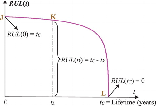
Let us consider a degradation trajectory D(t) of a system where a specific instant (or cycle) t_k is studied. The variable t_k denotes here the system age that is measured by the number of years (Figure 18). Referring to Figures 18 and 19, we can infer that at the system age t_k, the prognostic study must give the prediction of the failure instant t_C. Therefore, the RUL predicted here at the instant t_k has the following value: (12) In fact, at the beginning (t_k = 0) (point J) the system is intact, then the system failure probability P_r = 0, the chaotic factor in our prediction is zero (MChf = 0) since no chaos exists yet, and our knowledge of the undamaged and unharmed system is certain and complete (DOK = 1); therefore, If t_k = t_C (point L) the system is completely damaged, then RUL(t_C) = t_C − t_C = 0 and hence the system failure probability is one (P_r = 1). At this point, failure occurs. Hence, our knowledge of the completely worn-out system is certain (DOK = 1) and chaos has finished its harmful task so it is no more applicable (MChf = 0).

Figure 18. CPP and the prognostic of degradation.

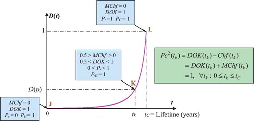
Figure 19. The prognostic of RUL.

If 0 < t_k < t_C (point K, where J < K < L), the occurrence probability of this instant and the prediction probability of D and RUL are both less than one and uncertain in (0 < P_r < 1). This is the consequence of non-zero chaotic factors affecting the system (MChf > 0). The DOK of the system subject to chaos is hence imperfect and is accordingly less than 1 in (0.5 < DOK < 1).

Additionally, by applying here the CPP paradigm, we can determine at any instant t_k and at any point inclusively and between J and L, the system D and RUL with certainty in the set since in we have Pc = 1 always.

Furthermore, we can define two complementary events E and with their respective probabilities by Then, let the probability in terms of the time t_k be equal to (13) where is the classical cumulative probability distribution function (CDF) of the random variable t.

Since , at an instant t = t_k, we have (14) Moreover, let us define two particular instants:

• t = t₀ = 0 which is assumed to be the initial time of functioning (system raw state) corresponding to D = D₀.

• And, t = t_C = the failure instant (system wear-out state) corresponding to the degradation D = D_C = 1.

Consequently, the boundary conditions are the following:

• For t = t₀ = 0, we have: D = D₀ ≈ 0 (the initial damage that may be nearly zero) and .

• For t = t_C we have: D = D_C = 1 and .

We note also that, since F(t_k) is defined as a cumulative probability function, then F(t_k) is a non-decreasing function that varies between 0 and 1. In addition, since RUL(t_k) = t_C − t_k and t_k is always increasing , RUL(t_k) is a non-increasing RUL function (Figure 19).

5.2. The new prognostic model (Beden, Abdullah, & Ariffin, 2009; Bidabad, Bidabad, & Mastorakis, 2014; Christensen, 2007; Cox, 1955; Fagin, Halpern, & Megiddo, 1990; Guan, Jha, & Liu, 2010; Huang, 2012; Husin, Rahman, Kadirgama, Noor, & Bakar, 2010; Ognjanović, Marković, Rašković, Doder, & Perović, 2012; Sankavaram et al., 2009; Stepić & Ognjanović, 2014; Weingarten, 2002; Wei, Qiu, Karimi, & Wang, 2014a, 2014b; Xiang & Liu, 2010; Youssef, 1994)

Let us present now the basic assumption of the new prognostic model. We consider first the CDF F(t) of the random time variable t as being equal to the degradation function itself, that means: (15) We note that we are dealing here with discrete random functions depending on the discrete random time t of pressure cycles.

This basic assumption is plausible since:

1. Both F and D are non-decreasing functions.

2. Both are cumulative functions starting from 0 and ending with 1.

3. Both functions are without measure units: F is an indicator quantifying chance and randomness, and D is an indicator quantifying degradation and system damage.

Then, we assume that the real system failure probability at the instant is equal to: (16) where

• the time of pressure cycles, and t₀ = 0 = the initial time of pressure cycles at the simulation beginning. It corresponds to a degradation D = D(t₀) = D₀ which is generally considered to be nearly equal to 0. Hence, since F(t_k) = D(t_k), F(t₀) = D(t₀) ≈ 0, but F(t₀) will be considered throughout this paper as being equal to zero;

• t₁ = the first pressure cycle time;

• … … … 

• t_k = the kth pressure cycle time;

• …  …  … 

• t_C = the time of pressure cycles till system failure = the critical number of pressure time. It corresponds to D = D_C = 1. It follows directly that F(t_C) = t_C = 1.

•  = the simulation magnifying factor that depends on the pressure profile. It is ψ₁ = 550.7 for the high-pressure mode (j = 1, mode 1), for the middle-pressure mode (j = 2, mode 2), and for the low-pressure mode (j = 3, mode 3).

Thus, initially we have Moreover, (17) where is the usual PDF. Knowing that, from classical probability theory, we have always: Therefore, we can deduce that: (18) This result is reasonable since is here a PDF (Figure 20).

Figure 20. P_r, degradation, and the CDF step function.

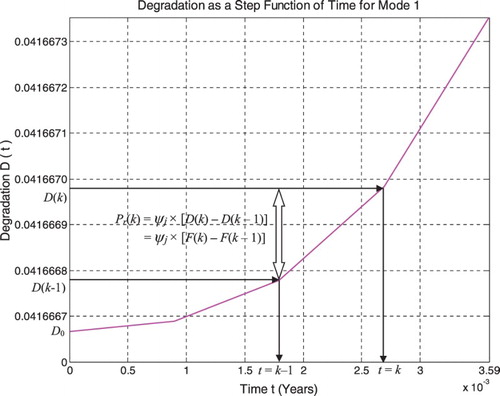
We can observe that D(t) = F(t) is a discrete CDF, where the amount of the jump is ; therefore, is a function of degradation and damage evolution (Figures 20 and 21). And we can realize from the previous calculations that is a PDF. Consequently, we can understand now that measures the probability of the system failure or degradation. Accordingly, what we have done here is that we have linked probability theory to degradation measure.

Note that and Thus, since the degradation is very flat near 0 and starts increasing with t, becoming very acute at t = t_C, near t_C, P_r is the greatest and is equal to 1 (Figures 21 and 22).

Figure 21. P_r as a function of degradation D(t).

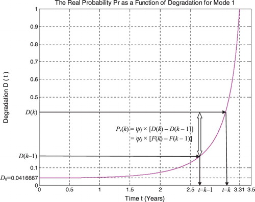
Figure 22. Degradation and P_r.

Furthermore, we have And This implies that (Figure 23): (19)

Figure 23. P_r, D, and RUL.

5.3. Analysis and extreme chaotic and random conditions

Although the analytic linear prognostic laws are deterministic and very well presented in Abou Jaoude et al. (2012a) there are general parameters that can be random and chaotic (such as temperature, humidity, geometry dimensions, material nature, water action, applied load location, atmospheric pressure, corrosion, and soil pressure and friction). Additionally, many variables in Equation (9) of degradation which are considered as deterministic can also have a stochastic behaviour, such as the initial crack length (potentially existing from the manufacturing process) and the applied pressure magnitude (due to the different pressure profile conditions). All those random factors, represented in the model by their mean values, affect the system and make its degradation function deviate from its calculated trajectory predefined by these deterministic laws. An updated follow-up of the degradation behaviour with time or cycle number, and which is subject to chaotic and non-chaotic effects, is done by due to its definition that evaluates the jumps in D. In fact, chaos modifies and affects all the environment and system parameters included in the degradation equation (Equation (9)). Consequently, chaos total effect on the pipelines contributes to shape the degradation curve D and is materialized by and counted in the pipeline system failure probability . Actually, quantifies the resultant of all the deterministic (non-random) and nondeterministic (random) factors and parameters which are included in the equation of D, which influence the system, and which determine the consequent final degradation curve. Accordingly, an accentuated effect of chaos on the system can lead to a bigger (or smaller) jump in the degradation trajectory and hence to a greater (or smaller) probability of failure . If, for example, due to extreme deterministic causes and random factors, D jumps directly from to 1 then RUL goes straight from t_C to 0 and consequently jumps instantly from 0 to 1: where t goes directly from 0 to t_C.

In the ideal extreme case, if the system never deteriorates (no pressure or stresses) and with zero chaotic causes and random factors, then the resultant of all the deterministic and nondeterministic effects is null (like in the system idle and isolated state). Consequently, the system stays indefinitely at and RUL remains equal to t_C. So accordingly the jump in D is always 0. Therefore, ideally, the probability of failure stays 0: where .

Figure 20 shows the real failure probability P_r(t) as a function of the random pipeline degradation step CDF in terms of the pressure cycles time t for mode 1.

Figure 21 shows the real failure probability P_r(t) as a function of the random pipeline degradation in terms of the pressure cycles time t for mode 1.

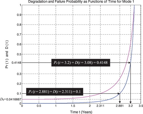
Figure 22 shows the real failure probability P_r(t) and the random pipeline degradation D(t) as functions of the number of the pressure cycles time t for mode 1.

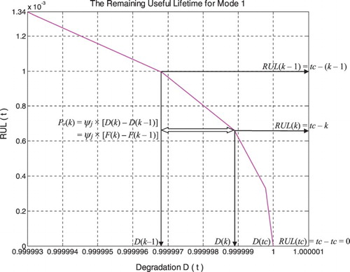
Figure 23 shows the real failure probability P_r(t) as a function of the random pipeline degradation D(t) and the random pipeline RUL(t) in terms of the pressure cycles time t (in years) for mode 1.

5.4. The evaluation of the new paradigm parameters

We can infer from what has been elaborated previously the following: (20) (21) (22) (23)

The DOK: (24) The chaotic factor: (25) Chf is null when P_r(N_k) = P_r(0) = 0 (point J) and when P_r(t_k) = P_r(t_C) = 1 (point L) (Figures 18 and 19).

The magnitude of the chaotic factor MChf: (26) MChf is null when P_r(t_k) = P_r(0) = 0 (point J) and when P_r(t_k) = P_r(t_C) = 1 (point L). (Figures 18 and 19)

At any instant t_k: , the probability expressed in the complex set is the following: (27) then, Pc(t_k) = P_r(t_k) + P_m(t_k)/i = P_r(t_k) + [1 − Pr(t_k)] = 1 always.

Hence, the prediction of D(t_k) and RUL(t_k) of the system in the set is permanently certain.

Let us consider thereafter the unburied pipeline system under its three pressure modes to simulate the cumulative distribution function F(t_k) = D(t_k) and to draw, to visualize, as well as to quantify all the CPP and prognostic parameters.

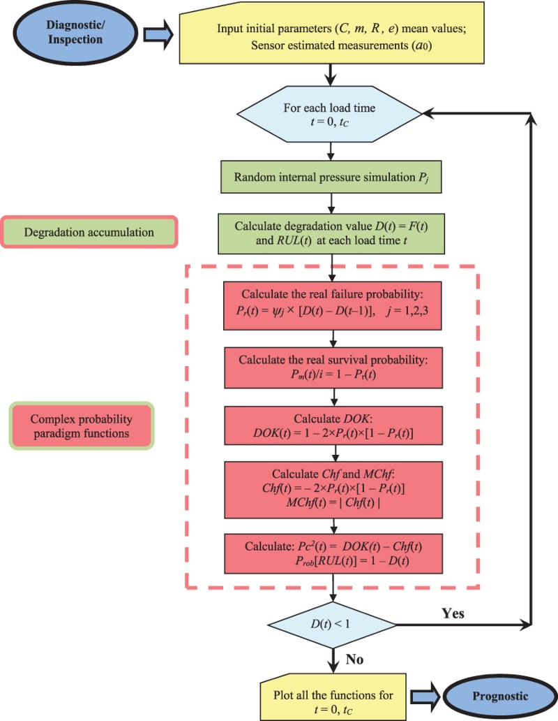
5.5. Flowchart of the complex probability analytic linear prognostic model

The following flowchart summarizes all the procedures of the proposed complex probability prognostic model:

6. Simulation of the new paradigm

In this section, the simulation of the novel prognostic model for the three modes of internal pressure will be done. Note that all the numerical values found in the paradigm functions analysis for the three modes of pressure were computed using the 64-Bit MATLAB version 2017 software.

6.1. The parameters’ analysis in the pipeline prognostic for Mode 1

RUL = [0, 3.31] is rescaled to [0, 1] in order to fit and represent it with all the CPP parameters and D which vary in [0, 1] on the same graph while having all of them as functions of the cycles time t = [0, 3.31].

We notice from Figures 24–29 that the DOK is maximum (DOK = 1) when MChf is minimum (MChf = 0) (points J & L) and that means when the magnitude of the chaotic factor (MChf) decreases our certain knowledge (DOK) in increases.

Figure 24. Pipeline degradation under linear damage law for high-pressure mode of excitation.

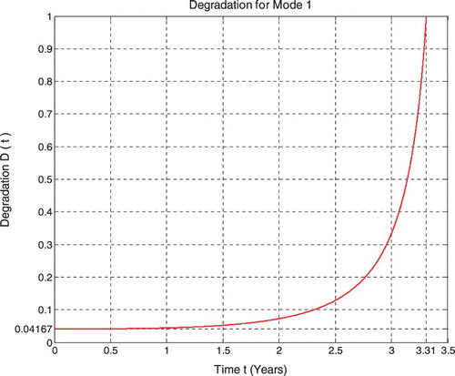
Figure 25. Pipeline RUL as a function of degradation for high-pressure mode of excitation.

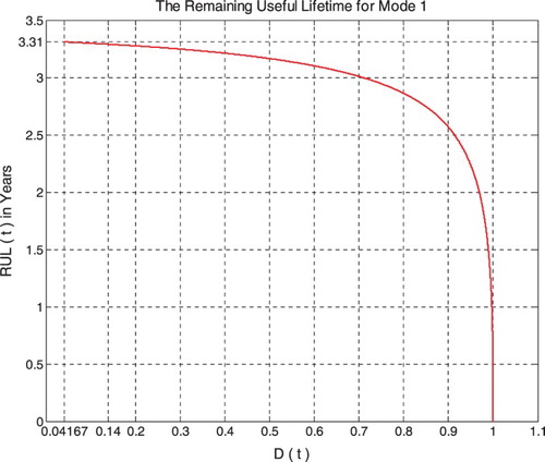
Figure 26. Degradation and CPP parameters for mode 1.

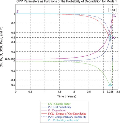
Figure 27. Degradation and CPP parameters with MChf for mode 1.

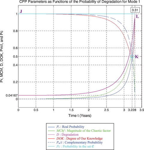
Figure 28. Degradation, rescaled RUL, and CPP parameters for mode 1.

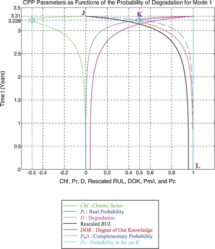
Figure 29. Degradation, rescaled RUL, and CPP parameters with MChf for mode 1.

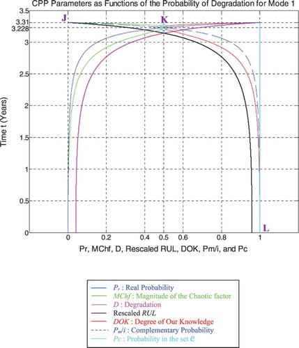
At the beginning (point J) P_r(t = t₀ = 0) = 0, the system is intact (nearly zero damage: D = D₀ = 0.04167 ≈ 0) and has zero chaotic factor (Chf(0) = MChf(0) = 0) before any usage, where at this instant (cycles number) DOK(0) = 1, RUL(0) = t_C − 0 = t_C = 3.31 years = t_C/1, and Rescaled[RUL(0)] = 0.95833. We have here the probability of the system collapse P_r(0) is 0; hence, this is the system raw state. At this point P_m/i(0) = 1, thus Pc(0) = P_r(0) + P_m/i(0) = 0 + 1 = 1 and Pc²(0) = DOK(0)− Chf(0) = DOK(0) + MChf(0) = 1 + 0 = 1 • Pc(0) = 1. Moreover, the complex random vector Z(0) = P_r(0) +P_m(0) = 0 + 1i = i • , just as predicted by the theory.

Afterwards t starts to increase (t > 0), then RUL(t) =t_C − t with P_r(t) = ψ₁ × [D(t) − D(t − 1)] ≠ 0, keeping constantly Pc(t) = P_r(t) + P_m/i(t) = 1 and Pc²(t) =DOK(t) − Chf(t) = DOK(t) + MChf(t) = 1 • Pc(t) = 1; therefore MChf starts to increase also during the system functioning due to the environment and intrinsic conditions thus leading to a decrease in DOK.

If t = t_C/2 = 3.31/2 = 1.655 years = half-life of the pipeline system, then RUL = t_C − t_C/2 = 1.655 years = t_C/2, Rescaled (RUL) = 0.94317, D = 0.05683, DOK =0.98813, Chf = −0.01187, MChf = 0.01187, P_r =0.005969, P_m/i = 0.994031, with Pc = P_r + P_m/i =0.005969 + 0.994031 = 1 and Pc² = DOK − Chf = DOK+ MChf = 0.98813 + 0.01187 = 1 • Pc = 1. Moreover, the complex probability vector Z = P_r + P_m = 0.005969+ 0.994031i • , just as predicted by CPP.

If D = 0.5 then t = 3.141 years, RUL = t_C − t = 0.169 years ≈ t_C/19.5858, Rescaled (RUL) = 0.5, DOK = 0.5846, Chf = −0.4154, MChf = 0.4154, P_r = 0.2943, P_m/i = 0.7057, with Pc = P_r + P_m/i = 0.2943 + 0.7057 = 1 and Pc² = DOK − Chf = DOK + MChf = 0.5846 + 0.4154 = 1 • Pc = 1. Moreover, Z = P_r + P_m = 0.2943 + 0.7057i • . At this point, both the rescaled RUL and D intersect. We can see that with the increase of t and hence the decrease of RUL, the probability of failure P_r increases also. Furthermore, notice in the last figure (Figure 29) the complete symmetry at the vertical axis D = 1/2 = degradation half-way to complete damage.

If t = 3.228 years (point K) both DOK (minimum) and MChf (maximum) reach 0.5 where RUL(N) = t_C − t = 3.31– 3.228 = 0.082 years ≈ t_C/40.3658, Rescaled (RUL) =  0.3179, D = 0.6821, P_r = 0.5, P_m/i = 0.5, and Chf = −0.5, with Pc = P_r + P_m/i = 0.5 + 0.5 = 1 and Pc² = DOK −  Chf = DOK + MChf = 0.5 + 0.5 = 1 • Pc = 1, as always. Moreover, Z = P_r + P_m = 0.5 + 0.5i • , just as expected. Thus, all the CPP parameters will intersect at the point K. We have here the maximum of chaos and the minimum of the system knowledge; therefore, the probability of the system crash is P_r = 1/2 = probability half-way to complete damage.

If D = 0.9 then t = 3.29 years, RUL = t_C − t = 0.02 years = t_C / 165.5, Rescaled (RUL) = 0.1, DOK = 0.7111, Chf = −0.2889, MChf = 0.2889, P_r = 0.8249, P_m/i =  0.1751, Pc = P_r + P_m/i = 0.8249 + 0.1751 = 1 and Pc² = DOK − Chf = DOK + MChf = 0.7111 + 0.2889 = 1 • Pc =1. Moreover, Z = P_r + P_m = 0.8249 + 0.1751i • . Here, since D = 0.9 which is very close to 1, then the failure probability P_r is very near to 1 since we will reach total damage very soon.

With the increase of the time of functioning, t reaches at the end t_C, MChf and Chf return to zero since chaos has finished its harmful task so it is no more applicable, DOK returns to 1 where we reach total damage (D = 1) at t = t_C = 3.31 years and hence the breakdown of the system (point L). At this last point, failure here is certain, this is the system wear-out state; therefore, P_r = 1, P_m/i = 0, RUL(t) = t_C − t = t_C − t_C = 0, Rescaled (RUL) = 0, with Pc = P_r + P_m/i = 1 + 0 = 1 and Pc² = DOK − Chf =DOK + MChf = 1 + 0 = 1 • Pc = 1. Thus, the logical consequence of the value of DOK(t_C) = 1 follows since our knowledge of the entirely deteriorated system is total and complete, just like DOK(t₀) = 1 where our knowledge of the entirely unharmed system is total and complete also. Moreover, Z = P_r + P_m = 1 + 0i = 1 • the square of the norm of the vector Z is , just as predicted by CPP.

We note that the same logic and analysis concerning the degradation, the RUL, as well as all the CPP parameters apply for all the three modes of pressure. In fact, the same consequences and results will be reached for the other two pressure modes, just like mode 1.

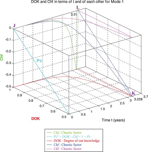
6.1.1. The complex probability cubes for Mode 1

In the first cube (Figure 30), the simulation of DOK and Chf as functions of each other and of the cycles time t for mode 1 of pressure can be seen. The line in cyan is the projection of Pc²(t) = DOK(t) − Chf(t) = 1 = Pc(t) on the plane t = 0. This line starts at the point J (DOK = 1, Chf = 0) when t = 0 years, reaches the point (DOK = 0.5, Chf = −0.5) when t = 3.228 years, and returns at the end to J (DOK = 1, Chf = 0) when t = t_C = 3.31 years. The other curves are the graphs of DOK(t) (red) and Chf(t) (green, blue, and pink) in different planes. Notice that they all have a minimum at the point K (DOK = 0.5, Chf = −0.5, t = 3.228 years). The point L corresponds to (DOK = 1, Chf = 0, t = t_C = 3.31 years). The three points J, K, L are the same as in Figures 26–29.

Figure 30. DOK and Chf in terms of t and of each other for mode 1.

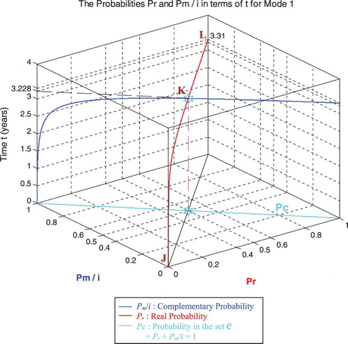
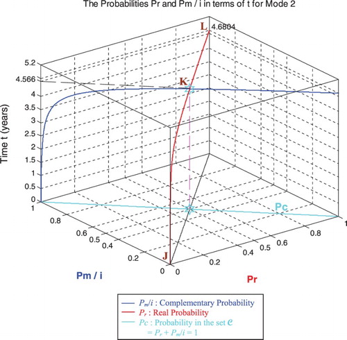
In the second cube (Figure 31), we can notice the simulation of the failure probability P_r(t) and its complementary real probability P_m/i(t) in terms of the cycles time t for mode 1 of pressure. The line in cyan is the projection of Pc²(t) = P_r(t) + P_m/i(t) = 1 = Pc(t) on the plane t = 0. This line starts at the point (P_r = 0, P_m/i = 1) and ends at the point (P_r = 1, P_m/i = 0). The red curve represents P_r(t) in the plane P_r(t) = P_m/i(t). This curve starts at the point J (P_r = 0, P_m/i = 1, t = 0 years), reaches the point K (P_r = 0.5, P_m/i = 0.5, t = 3.228 years), and gets at the end to L (P_r = 1, P_m/i = 0, t = t_C = 3.31 years). The blue curve represents P_m/i(t) in the plane P_r(t) + P_m/i(t) = 1. Notice the importance of the point K which is the intersection of the red and blue curves at t = 3.228 years and when P_r(t) = P_m/i(t) = 0.5. The three points J, K, L are the same as in Figures 26–29.

Figure 31. P_r and P_m/i in terms of t and of each other for mode 1.

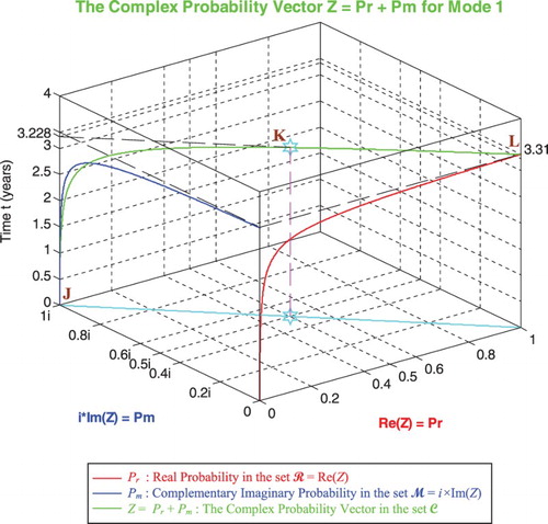
In the third cube (Figure 32), we can notice the simulation of the complex random vector Z(t) in as a function of the real failure probability P_r(t) = Re(Z) in and of its complementary imaginary probability P_m(t) = i × Im(Z) in , and this in terms of the cycles time t for mode 1 of pressure. The red curve represents P_r(t) in the plane P_m(t) = 0 and the blue curve represents P_m(t) in the plane P_r(t) = 0. The green curve represents the complex probability vector Z(t) = P_r(t) + P_m(t) = Re(Z) + i × Im(Z) in the plane P_r(t) = iP_m(t) + 1. The curve of Z(t) starts at the point J (P_r = 0, P_m = i, t = 0 years) and ends at the point L (P_r = 1, P_m = 0, t = t_C = 3.31 years). The line in cyan is P_r(0) = iP_m(0) + 1 and it is the projection of the Z(t) curve on the complex probability plane whose equation is t = 0 years. This projected line starts at the point J (P_r = 0, P_m = i, t = 0 years) and ends at the point (P_r = 1, P_m = 0, t = 0 years). Notice the importance of the point K corresponding to t = 3.228 years and when P_r = 0.5 and P_m = 0.5i. The three points J, K, L are the same as in Figures 26–29. Note that similar cubes can be drawn for modes 2 and 3 with their corresponding t_C and points J, K, and L.

Figure 32. The complex probability vector Z in terms of t for mode 1.

6.2. The parameters’ analysis in the pipeline prognostic for Mode 2:

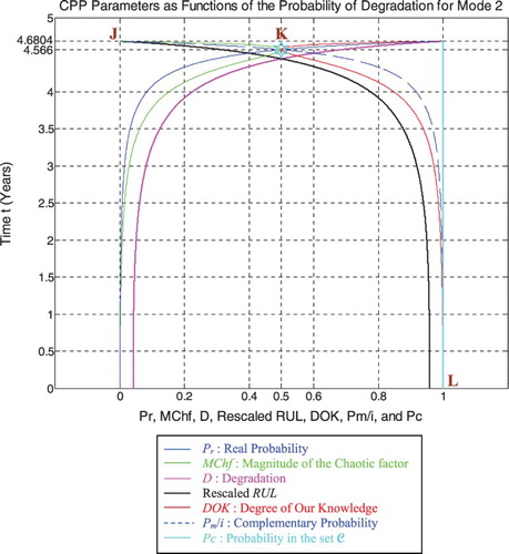
Just like for mode 1 simulations, RUL = [0, 4.6804] is rescaled to [0, 1] in order to fit and represent it with all the CPP parameters and D which vary in [0, 1] on the same graph while having all of them as functions of the cycles time t = [0, 4.6804].

We note from Figures 33–38 that the DOK is maximum (DOK = 1) when MChf is minimum (MChf = 0) (points J & L) and that means when the magnitude of the chaotic factor (MChf) decreases our certain knowledge (DOK) in increases.

Figure 33. Pipeline degradation under linear damage law for middle-pressure mode of excitation.

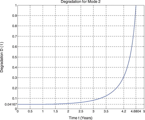
Figure 34. Pipeline RUL as a function of degradation for middle-pressure mode of excitation.

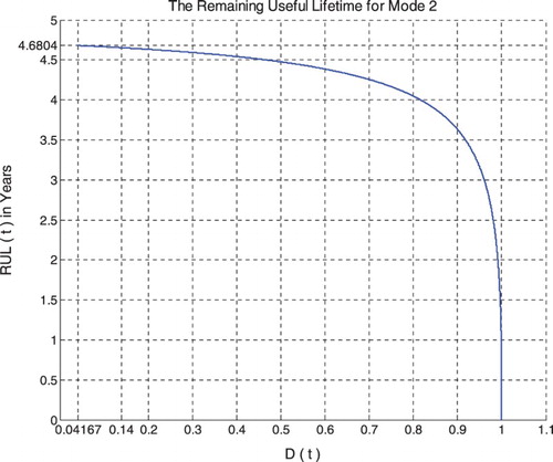
Figure 35. Degradation and CPP parameters for mode 2.

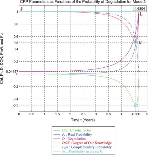
Figure 36. Degradation and CPP parameters with MChf for mode 2.

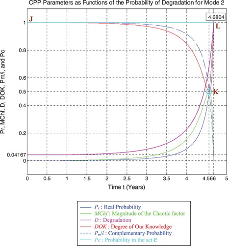
Figure 37. Degradation, rescaled RUL, and CPP parameters for mode 2.

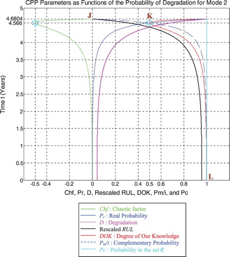
Figure 38. Degradation, rescaled RUL, and CPP parameters with MChf for mode 2.

At the beginning (point J) P_r(t = t₀ = 0) = 0, the system is intact (nearly zero damage: D = D₀ = 0.04167 ≈ 0) and has zero chaotic factor (Chf (0) = MChf(0) = 0) before any usage. At this instant (cycles number) DOK(0) = 1 and RUL(0) = t_C − 0 = t_C = 4.6804 years =t_C/1, Rescaled[RUL(0)] = 0.95833. Here P_m/i(0) = 1, with Pc(0) = P_r(0) + P_m/i(0)=0 +1=1 and Pc²(0)=DOK(0)− Chf(0) =DOK(0) + MChf(0) = 1 + 0 = 1 • Pc(0) = 1. Moreover, the complex random vector Z(0) = P_r(0) +P_m(0) = 0 + 1i = i • , just as predicted by the theory.

Afterwards t starts to increase (t > 0), then RUL(t) =t_C − t with P_r(t) = ψ₂ × [D(t) − D(t − 1)] ≠ 0, keeping constantly Pc(t) = P_r(t) + P_m/i(t) = 1 and Pc²(t) =DOK(t) − Chf(t) = DOK(t) + MChf(t) = 1 • Pc(t) = 1, therefore MChf starts to increase also during the system functioning due to the environment and intrinsic conditions thus leading to a decrease in DOK.

If t = t_C/2 = 4.6804/2 = 2.3402 years = half-life of the pipeline system, then RUL = t_C − t_C/2 = 4.6804 − 2.3402 = 2.3402 years = t_C/2, Rescaled (RUL) = 0.94317, D = 0.05683, DOK = 0.98819, Chf = −0.01181, MChf =0.01181, P_r = 0.005941, P_m/i = 0.994059, with Pc = P_r +P_m/i = 0.005941 + 0.994059 = 1 and Pc² = DOK −Chf = DOK + MChf = 0.98819 + 0.01181 = 1 • Pc = 1. Moreover, the complex probability vector Z = P_r + P_m =0.005941 + 0.994059i • , just as predicted.

If D = 0.5 then t = 4.442 years, RUL = t_C − t = 0.2384 years ≈ t_C/19.6325, Rescaled(RUL) = 0.5, DOK = 0.5849, Chf = −0.4151, MChf = 0.4151, P_r = 0.2940, P_m/i =0.7060, with Pc = P_r + P_m/i = 0.2940 + 0.7060 = 1 and Pc² = DOK − Chf = DOK + MChf = 0.5849 + 0.4151 = 1 • Pc = 1. Moreover, Z = P_r + P_m = 0.2940 + 0.7060i •. At thispoint, both the rescaled RUL and D intersect. We can see that with the increase of t and hence the decrease of RUL, the probability of failure P_r increases also. Furthermore, notice in the last figure (Figure 38) the complete symmetry at the vertical axis D = 1/2 = degradation half-way to complete damage.

If t = 4.566 years (point K) both DOK (minimum) and MChf (maximum) reach 0.5 where RUL(t) = t_C − t = 4.6804 − 4.566 = 0.1144 years ≈ t_C/40.9125, Rescaled(RUL) = 0.3152, D = 0.6848, P_r = 0.5, P_m/i = 0.5, and Chf = −0.5, with Pc = P_r + P_m/i = 0.5 + 0.5 = 1, and Pc² = DOK − Chf = DOK + MChf = 0.5 + 0.5 = 1 •Pc =1, as always. Moreover, Z = P_r + P_m = 0.5 + 0.5i • , just as expected. Thus, all the CPP parameters will intersect at the point K. We have here the maximum of chaos and the minimum of the system certain knowledge; therefore, the probability of the system crash is P_r = 1/2 = probability half-way to complete damage. We note that relatively to mode 1 (high-pressure conditions), the point K in Figures 35–38 is no more at (3.228, 0.5) but shifted to the right and is now at (4.566, 0.5) since the degradation curve for mode 2 (middle-pressure conditions) is naturally different. Hence, DOK, Chf, and MChf are more skewed to the left relatively to mode 1.

If D = 0.9 then t = 4.652 years, RUL = t_C − t = 0.0284 years ≈ t_C/164.8028, Rescaled (RUL) = 0.1, DOK = 0.7056, Chf = −0.2944, MChf = 0.2944, P_r = 0.8206, P_m/i =0.1794, Pc = P_r + P_m/i = 0.8206 + 0.1794 = 1 and Pc² =DOK − Chf = DOK + MChf =0.7056+ 0.2944= 1 • Pc = 1. Moreover, Z = P_r + P_m = 0.8206 + 0.1794i • . Here, since D =0.9 which is very close to 1, then the failure probability P_r is very near to 1 since we will reach total damage very soon.

With the increase of the time of functioning, t reaches at the end t_C, MChf and Chf return to zero since chaos has finished its harmful task so it is no more applicable, DOK returns to 1, where we reach total damage (D = 1) at t = t_C = 4.6804 years and hence the breakdown of the system (point L). At this last point, failure here is certain, this is the system wear-out state; therefore, P_r = 1, P_m/i = 0, RUL(t) = t_C − t = t_C − t_C = 0, Rescaled (RUL) = 0, with Pc = P_r + P_m/i = 1 + 0 = 1 and Pc² =DOK − Chf = DOK + MChf = 1 + 0 = 1 • Pc = 1. Thus, the logical consequence of the value of DOK(t_C) = 1 follows since our knowledge of the entirely deteriorated system is total and complete, just like DOK(t₀) = 1, where our knowledge of the entirely unharmed system is total and complete also. Moreover, Z = P_r + P_m = 1 + 0i = 1 • the square of the norm of the vector Z is , just as predicted by CPP.

We note that the same logic and analysis for mode 1 of pressure are applied to mode 2 of pressure concerning the degradation, the RUL, as well as all the CPP parameters. In fact, the same consequences and results will be reached for pressure mode 3, just like the first two modes.

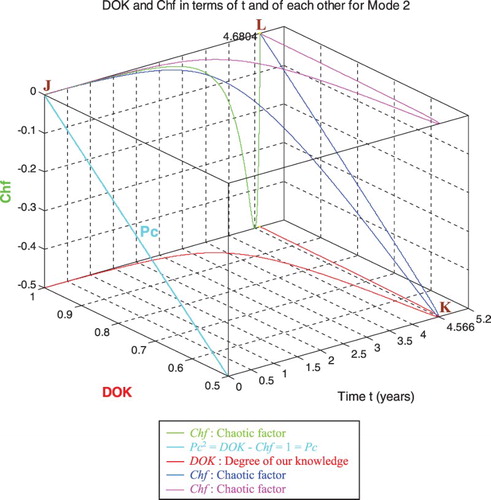
6.2.1. The complex probability cubes for Mode 2

In the first cube (Figure 39), the simulation of DOK and Chf as functions of each other and of the cycles time t for mode 2 of pressure can be seen. The line in cyan is the projection of Pc²(t) = DOK(t) − Chf(t) = 1 = Pc(t) on the plane t = 0. This line starts at the point J (DOK = 1, Chf = 0) when t = 0 years, reaches the point (DOK = 0.5, Chf = −0.5) when t = 4.566 years, and returns at the end to J (DOK = 1, Chf = 0) when t = t_C = 4.6804 years. The other curves are the graphs of DOK(t) (red) and Chf(t) (green, blue, and pink) in different planes. Notice that they all have a minimum at the point K (DOK = 0.5, Chf = −0.5, t = 4.566 years). The point L corresponds to (DOK = 1, Chf = 0, t = t_C = 4.6804 years). The three points J, K, L are the same as in Figures 35–38.

Figure 39. DOK and Chf in terms of t and of each other for mode 2.

In the second cube (Figure 40), we can notice the simulation of the failure probability P_r(t) and its complementary real probability P_m/i(t) in terms of the cycles number t for mode 2 of pressure. The line in cyan is the projection of Pc²(t) = P_r(t) + P_m/i(t) = 1 = Pc(t) on the plane t = 0. This line starts at the point (P_r = 0, P_m/i = 1) and ends at the point (P_r = 1, P_m/i = 0). The red curve represents P_r(t) in the plane P_r(t) = P_m/i(t). This curve starts at the point J (P_r = 0, P_m/i = 1, t = 0 years), reaches the point K (P_r = 0.5, P_m/i = 0.5, t = 4.566 years), and gets at the end to L (P_r = 1, P_m/i = 0, t = t_C = 4.6804 years). The blue curve represents P_m/i(t) in the plane P_r(t) + P_m/i(t) = 1. Notice the importance of the point K which is the intersection of the red and blue curves at t = 4.566 years and when P_r(t) = P_m/i(t) = 0.5. The three points J, K, L are the same as in Figures 35–38.

Figure 40. P_r and P_m/i in terms of t and of each other for mode 2.

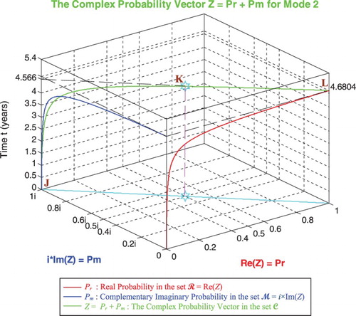
In the third cube (Figure 41), we can notice the simulation of the complex random vector Z(t) in as a function of the real failure probability P_r(t) = Re(Z) in and of its complementary imaginary probability P_m(t) = i × Im(Z) in , and this in terms of the cycles time t for mode 2 of pressure. The red curve represents P_r(t) in the plane P_m(t) = 0 and the blue curve represents P_m(t) in the plane P_r(t) = 0. The green curve represents the complex probability vector Z(t) = P_r(t) + P_m(t) = Re(Z) + i × Im(Z) in the plane P_r(t) = iP_m(t) + 1. The curve of Z(t) starts at the point J (P_r = 0, P_m = i, t = 0 years) and ends at the point L (P_r = 1, P_m = 0, t = t_C = 4.6804 years). The line in cyan is P_r(0) = iP_m(0) + 1 and it is the projection of the Z(t) curve on the complex probability plane whose equation is t = 0 years. This projected line starts at the point J (P_r = 0, P_m = i, t = 0 years) and ends at the point (P_r = 1, P_m = 0, t = 0 years). Notice the importance of the point K corresponding to t = 4.566 years and when P_r = 0.5 and P_m = 0.5i. The three points J, K, L are the same as in Figures 35–38. Note that similar cubes can be drawn for mode 3 with its corresponding t_C and points J, K, and L.

Figure 41. The complex probability vector Z in terms of t for mode 2.

6.3. The parameters’ analysis in the pipeline prognostic for Mode 3

Just like for modes 1 and 2 simulations, RUL = [0, 6.8493] is rescaled to [0, 1] in order to fit and represent it with all the CPP parameters and D which vary in [0, 1] on the same graph while having all of them as functions of the cycles time t = [0, 6.8493].

We note from Figures 42–47 that the DOK is maximum (DOK = 1) when MChf is minimum (MChf = 0) (points J & L) and that means when the magnitude of the chaotic factor (MChf) decreases our certain knowledge (DOK) in increases.

Figure 42. Pipeline degradation under linear damage law for low-pressure mode of excitation.

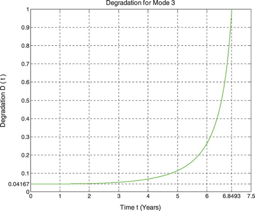
Figure 43. Pipeline RUL as a function of degradation for low-pressure mode of excitation.

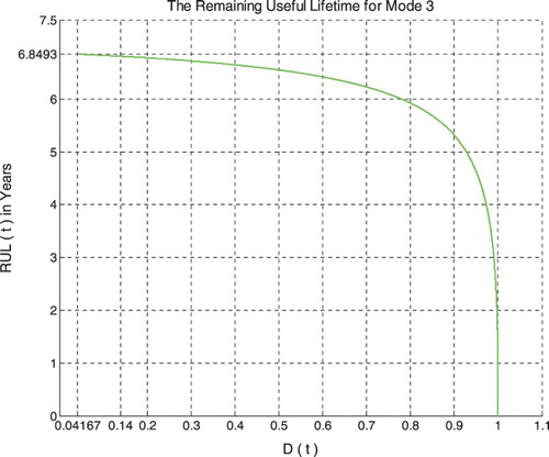
Figure 44. Degradation and CPP parameters for mode 3.

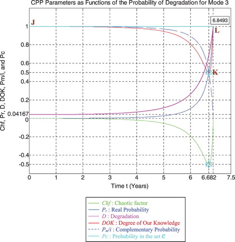
Figure 45. Degradation and CPP parameters with MChf for mode 3.

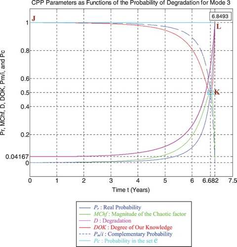
Figure 46. Degradation, rescaled RUL, and CPP parameters for mode 3.

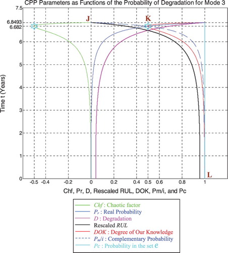
Figure 47. Degradation, rescaled RUL, and CPP parameters with MChf for mode 3.

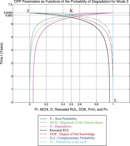
At the beginning (point J) P_r(t = t₀ = 0) = 0, the system is intact (nearly zero damage: D = D₀ = 0.04167 ≈ 0) and has zero chaotic factor (Chf(0) = MChf(0) = 0) before any usage, where at this instant (cycles number) DOK(0) =1, RUL(0) = t_C − 0 = t_C = 6.8493 years = t_C/1, andRescaled [RUL(0)] = 0.95833. Here P_m/i(0) = 1 withPc(0) = P_r(0) + P_m/i(0) = 0 + 1 = 1 and Pc²(0) =DOK(0) − Chf(0) = DOK(0) + MChf(0) = 1 + 0 = 1 • Pc(0)= 1. Moreover, the complex random vector Z(0) = P_r(0) +P_m(0) = 0 + 1i = i • ,just as predicted by the theory.

Afterwards t starts to increase (t > 0), then RUL(t) =t_C − t with P_r(t) = ψ₃ × [D(t) − D(t − 1)] ≠ 0, keeping constantly Pc(t) = P_r(t) + P_m/i(t) = 1 and Pc²(t) =DOK(t) − Chf(t) = DOK(t) + MChf(t) = 1 • Pc(t) = 1; therefore, MChf starts to increase also during the system functioning due to the environment and intrinsic conditions, thus leading to a decrease in DOK.

If t = t_C/2 = 6.8493/2 = 3.42465 years = half-life of the pipeline system, then RUL = t_C − t_C/2 = 6.8493 −3.42465 = 3.42465 years = t_C/2, Rescaled (RUL) =0.94317, D = 0.05683, DOK = 0.98819, Chf = −0.01181, MChf = 0.01181, P_r = 0.005939, P_m/i = 0.994061, with Pc = P_r + P_m/i = 0.005939 + 0.994061 = 1 and Pc² =DOK − Chf = DOK + MChf = 0.98819 + 0.01181 = 1 • Pc = 1. Moreover, the complex probability vector Z = P_r + P_m = 0.005939 + 0.994061i • .

If D = 0.5 then t = 6.5 years, RUL = t_C − t = 0.3493 years ≈ t_C/19.6086, Rescaled (RUL) = 0.5, DOK = 0.5852, Chf = −0.4148, MChf = 0.4148, P_r = 0.2936, P_m/i =0.7064, with Pc = P_r + P_m/i = 0.2936 + 0.7064 = 1 and Pc² = DOK − Chf = DOK + MChf = 0.5852 + 0.4148 = 1 • Pc = 1. Moreover, Z = P_r + P_m = 0.2936 + 0.7064i •. At this point, both the rescaled RUL and D intersect. We can see that with the increase of t and consequently the decrease of RUL, the probability of failure P_r increases also. Furthermore, notice in the last figure (Figure 47), the complete symmetry at the vertical axis D = 1/2 = degradation half-way to complete damage.

If t = 6.682 years (point K) both DOK (minimum) and MChf (maximum) reach 0.5 where RUL(t) = t_C − t = 6.8493–6.682 = 0.1673 years ≈ t_C/40.9402, Rescaled (RUL) =0.3148, D = 0.6852, P_r = 0.5, P_m/i = 0.5, and Chf = −0.5 with Pc = P_r + P_m/i = 0.5 + 0.5 = 1 and Pc² = DOK −Chf = DOK + MChf = 0.5 + 0.5 = 1 • Pc = 1, as always. Moreover, the complex probability vector Z = P_r + P_m =0.5 + 0.5i • , just as expected. Hence, all the CPP parameters will intersect at the point K. We have here the maximum of chaos and the minimum of the system knowledge; therefore, the probability of the system crash is P_r = 1/2 = probability half-way to complete damage. We note that relatively to mode 1 (high-pressure conditions) and mode 2 (middle-pressure conditions), the point K in Figures 44–47 is no more at (3.228, 0.5) or (4.566, 0.5) but shifted more to the right and is now at (6.682, 0.5) since the degradation curve for mode 3 (low-pressure conditions) is eventually different. Hence, DOK, Chf, and MChf are more negatively skewed relatively to modes 1 and 2.

If D = 0.9 then t = 6.808 years, RUL = t_C − t = 0.0413 years ≈ t_C / 165.8426, Rescaled (RUL) = 0.1, DOK = 0.7052, Chf = −0.2948, MChf = 0.2948, P_r = 0.8203, P_m/i =0.1797, with Pc = P_r + P_m/i = 0.8203 + 0.1797 = 1 and Pc² = DOK − Chf = DOK + MChf = 0.7052 + 0.2948 = 1 • Pc = 1. Moreover, Z = P_r + P_m = 0.8203 + 0.1797i • , just as expected. Here, since D = 0.9 which is very close to 1, then the failure probability P_r is very near to 1 since we will reach total damage very soon.

With the increase of the time of functioning, t reaches at the end t_C, MChf and Chf return to zero since chaos has finished its harmful task so it is no more applicable, DOK returns to 1 where we reach total damage (D = 1) at t = t_C = 6.8493 years and hence the breakdown of the system (point L). At this last point, failure here is certain, this is the system wear-out state; therefore, P_r = 1, P_m/i = 0, RUL(t) = t_C − t = t_C − t_C = 0, Rescaled (RUL) = 0, with Pc = P_r + P_m/i = 1 + 0 = 1 and Pc² =DOK − Chf = DOK + MChf = 1 + 0 = 1 • Pc = 1. Thus, the logical consequence of the value of DOK(t_C) = 1 follows since our knowledge of the entirely deteriorated system is total and complete, just like DOK(t₀) = 1 where our knowledge of the entirely unharmed system is total and complete also. Moreover, Z = P_r + P_m = 1 + 0i = 1 • the square of the norm of the vector Z is , just as predicted by CPP.

6.3.1. The complex probability cubes for Mode 3

In the first cube (Figure 48), the simulation of DOK and Chf as functions of each other and of the cycles' time t for mode 3 of pressure can be seen. The line in cyan is the projection of Pc²(t) = DOK(t) − Chf(t) = 1 = Pc(t) on the plane t = 0. This line starts at the point J (DOK = 1, Chf = 0) when t = 0 years, reaches the point (DOK = 0.5, Chf = −0.5) when t = 6.682 years, and returns at the end to J (DOK = 1, Chf = 0) when t = t_C = 6.8493 years. The other curves are the graphs of DOK(t) (red) and Chf(t) (green, blue, pink) in different planes. Notice that they all have a minimum at the point K (DOK = 0.5, Chf = −0.5, t = 6.682 years). The point L corresponds to (DOK = 1, Chf = 0, t = t_C = 6.8493 years). The three points J, K, L are the same as in Figures 44–47.

Figure 48. DOK and Chf in terms of t and of each other for mode 3.

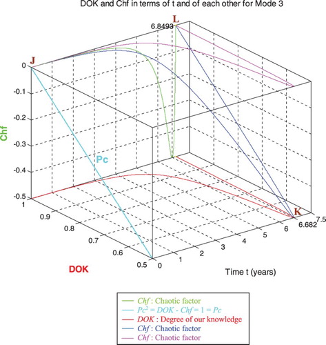
In the second cube (Figure 49), we can notice the simulation of the failure probability P_r(t) and its complementary real probability P_m/i(t) in terms of the cycles time t for mode 3 of pressure. The line in cyan is the projection of Pc²(t) = P_r(t) + P_m/i(t) = 1 = Pc(t) on the plane t = 0. This line starts at the point (P_r = 0, P_m/i = 1) and ends at the point (P_r = 1, P_m/i = 0). The red curve represents P_r(t) in the plane P_r(t) = P_m/i(t). This curve starts at the point J (P_r = 0, P_m/i = 1, t = 0 years), reaches the point K (P_r = 0.5, P_m/i = 0.5, t = 6.682 years), and gets at the end to L (P_r = 1, P_m/i = 0, t = t_C = 6.8493 years). The blue curve represents P_m/i(t) in the plane P_r(t) + P_m/i(t) = 1. Notice the importance of the point K which is the intersection of the red and blue curves at t = 6.682 years and when P_r(t) = P_m/i(t) = 0.5. The three points J, K, L are the same as in Figures 44–47.

Figure 49. P_r and P_m/i in terms of t and of each other for mode 3.

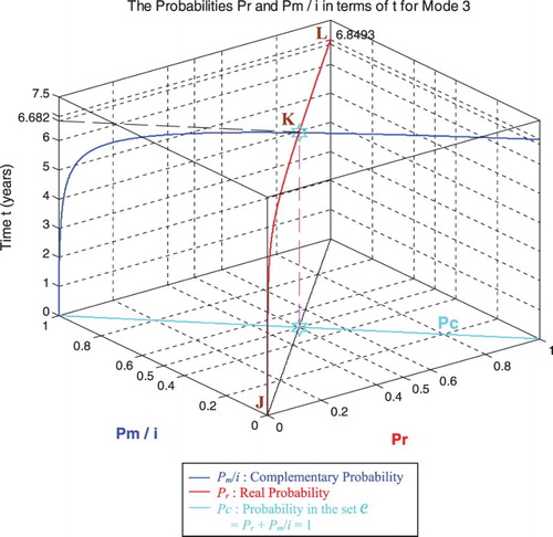
In the third cube (Figure 50), we can notice the simulation of the complex random vector Z(t) in as a function of the real failure probability P_r(t) = Re(Z) in and of its complementary imaginary probability P_m(t) = i × Im(Z) in , and this in terms of the cycles time t for mode 3 of pressure. The red curve represents P_r(t) in the plane P_m(t) = 0 and the blue curve represents P_m(t) in the plane P_r(t) = 0. The green curve represents the complex probability vector Z(t) = P_r(t) + P_m(t) = Re(Z) + i × Im(Z) in the plane P_r(t) = iP_m(t) + 1. The curve of Z(t) starts at the point J (P_r = 0, P_m = i, t = 0 years) and ends at the point L (P_r = 1, P_m = 0, t = t_C = 6.8493 years). The line in cyan is P_r(0) = iP_m(0) + 1 and it is the projection of the Z(t) curve on the complex probability plane whose equation is t = 0 years. This projected line starts at the point J (P_r = 0, P_m = i, t = 0 years) and ends at the point (P_r = 1, P_m = 0, t = 0 years). Notice the importance of the point K corresponding to t = 6.682 years and when P_r = 0.5 and P_m = 0.5i. The three points J, K, L are the same as in Figures 44–47.

Figure 50. The complex probability vector Z in terms of t for mode 3.

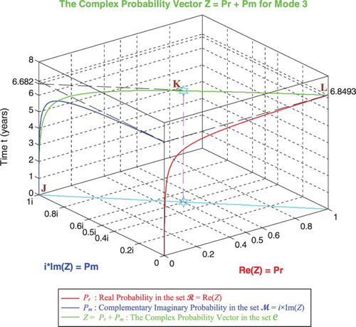
6.4. The parameters’ visualization in the pipeline prognostic for the three modes

Furthermore, the following simulations (Figures 51–56) recapitulate all the previous Figures 24–50. They are three-in-one figures.

Figure 51. Pipeline degradation under linear damage law for the three modes of pressure excitation.

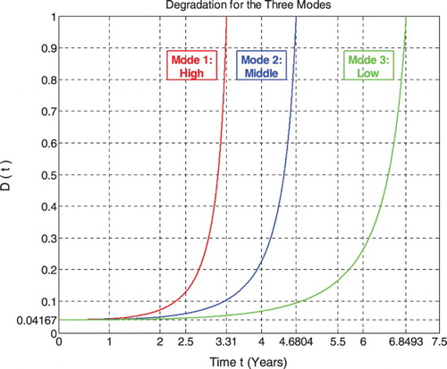
Figure 52. Pipeline RUL as a function of degradation for the three modes of pressure excitation.

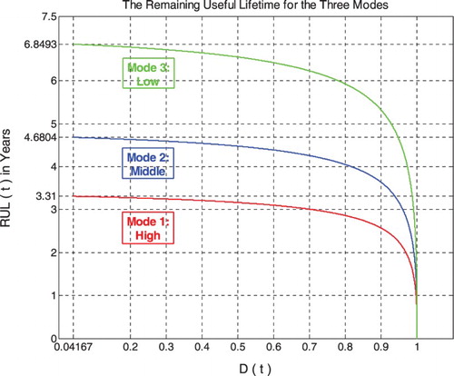
Figure 53. Degradation and CPP parameters for the three modes.

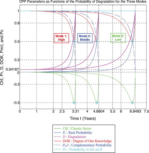
Figure 54. Degradation and CPP parameters with MChf for the three modes.

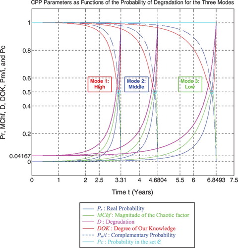
Figure 55. Degradation, rescaled RUL, and CPP parameters for the three modes.

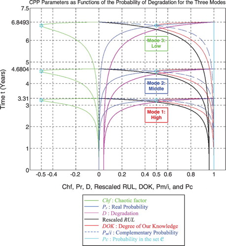
Figure 56. Degradation, rescaled RUL, and CPP parameters with MChf for the three modes.

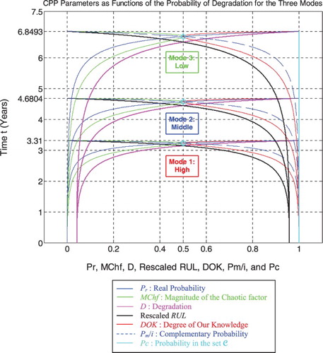
6.5. Final analysis

In this section, all the obtained data and achieved simulations will be interpreted, a final analysis will be done, and the novel general prognostic equations will be presented.

6.5.1. Explanation and the general prognostic equations

Firstly, probability theory represented by the CDF F(t) was linked with prognostic represented by the degradation D(t) by supposing that F(t) = D(t) and the justification for this assumption was given. In doing so, the deterministic D(t) taken from deterministic analytic linear prognostic becomes a nondeterministic CDF. Thus, the discrete and deterministic variable of pressure cycles time t becomes a discrete random variable. Therefore, the resultant of all the factors acting on the pipeline which was deterministic becomes a random resultant since D(t) measures now the pipeline random degradation as a function of the random cycles time t. Hence, all the exact parameters’ values of the D(t) equation (9) become now mean values of the random factors affecting the system and are represented by PDFs as functions of the random variable of pressure cycles time t (Refer to paragraph 4.5). In fact, this is the real-world case where randomness is omnipresent in one form or another. What we experience and consider as a deterministic phenomenon is nothing in reality but an approximation and a simplification of an actual stochastic and chaotic experiment due to the impact of a huge number of deterministic and nondeterministic factors and forces (a lottery machine is a good example).

Consequently, an updated follow-up of the random degradation behaviour with time or cycle number, and which is subject to chaotic and non-chaotic effects, is done by the quantity due to its definition that evaluates the jumps in the stochastic degradation CDF D(t). Hence, Referring to classical probability theory, this makes the system probability of failure at t = t_k, with and , just like any PDF.

In addition, in the simulations a constant and very small increments in t have been taken, which lead to very small increments in D and hence in . So by multiplying those very small jumps in D by a simulation magnifying factor that we called : for the high-pressure mode (j = 1, mode 1), for the middle-pressure mode (j = 2, mode 2), and for the low-pressure mode (j = 3, mode 3). So we get: if t tends to t₀ = 0 then tends to 0, and if t tends to t_C then tends to 1, so and as if were a CDF although mathematically speaking it is not at all. Thus, since is not cumulative, it is just times the probability of failure at t = t_k. Hence, in the simulations, becomes now the probability that the system failure occurs at t = t_k.

Therefore,  =P_rob(t = 0 or t = 1 or t = 2 or … or t = t_k) = sum of all failure probabilities between 0 and t_k = probability that failure will occur somewhere between 0 and t_k. So if t_k = 0 then  = probability that failure will occur at t = 0 and before. If t_k = t_C then  = sum of all failure probabilities between 0 and t_C = probability that failure will occur somewhere between 0 and t_C. If t_k > t_C then  = probability that failure will occur beyond t_C. We can see that failure probability increases with the increase of the pressure cycles time t_k until at the end it becomes 1 when .

Hence, If and then: This implies that and If and then the prognostic equation in the new model is (28) for any mode j of pressure profile and with .

In the general prognostic case, if we have the system failure PDF then we can include it in Equation (28) above and determine degradation and vice versa. Then, all the other model CPP functions (Chf, MChf, DOK, Z, P_r, P_m, P_m/i, Pc) will follow. This would be our new prognostic model general equation: (29) Additionally, in the three pressure modes’ simulations, and by applying CPP to the pipeline prognostic, we succeeded in the novel prognostic model to quantify in (our real laboratory) both our certain knowledge represented by DOK and chaos represented by Chf and MChf. These three CPP parameters are caused and evaluated by the resultant of all the deterministic (non-random) and nondeterministic (random) factors affecting the pipeline system. Knowing that, in the new model, the factors’ resultant effect on D and RUL is concretized by the jumps in their curves and is accordingly measured and expressed in by P_r and in by P_m. As defined in CPP, is an imaginary extension of the real probability set and the complex set is the sum of both probability sets; hence, . Since P_m = i(1 − P_r) then it is the complementary probability in of P_r. So if P_r is defined as the system failure probability in at the pressure cycles time t = t_k, then P_m is the corresponding probability in the set that the system failure will not occur at the same pressure time t = t_k. Thus, P_m is the associated probability in the set of the system survival at t = t_k. Accordingly, P_m/i = 1 − P_r is the associated probability but in the set of the system survival at the same pressure cycles time. From classical probability theory we know that the sum in of both complementary probabilities is surely 1. This sum is nothing but P_C which is equal to P_r + P_m/i = P_r + (1 − P_r) = 1 always. The sum in of both complementary probabilities is the complex random number and vector Z which is equal to P_r + P_m = P_r + i(1 − P_r). And as it was shown and illustrated in the complex probability cubes paragraphs, we understand that Z is the sum in of the real failure probability and of the imaginary survival probability in the complex probability plane whose equation is P_r(t) = iP_m(t) + 1 for , , . What is interesting is that the square of the norm of Z which is is nothing but DOK, as it was proved in CPP and in the new model. Moreover, since MChf = −2iP_rP_m = 2P_rP_m/i, then it is twice the product in of both the failure probability and the survival probability and it measures the magnitude of chaos since it is always zero or positive. All these facts are shown and proved in all the simulations.

From all the above we can conclude that since D(t) is a CDF, the factors’ resultant is random, the jumps in D are the failure probabilities , then we are dealing with a random experiment, thus the natural appearance of Chf, MChf, DOK, Z, and hence Pc. So we get (30) (31) (32) (33) (34)

Furthermore, in the new model, we have Note that, since t and D are random then RUL is also a random function of t. Thus, we have in the set : (35)

Then, we get always: everywhere.

This implies that: And .

Hence, we reach a new and general prognostic equation for RUL. If and then: (36) (37)

for any mode j of pressure profile.

In the ideal case, if all the factors are 100% deterministic, then we have in : the probability of failure for is 0 and is 1 for ; accordingly the probability of system survival for is 1 and is 0 for , since certain failure will occur only at . So degradation is determined surely everywhere in and its CDF is replaced by a deterministic function and curve. Therefore, chaos is null and hence Chf = MChf = 0 and DOK = 1 always for all . Thus, and .

Consequently, at each instant t in the novel prognostic model, the random D(t) and RUL(t) are certainly predicted in the complex set with Pc² = DOK − Chf = DOK +MChf maintained as equal to one through a continuous compensation between DOK and Chf. This compensation is from the instant t = 0 where D(t) = D₀ = 0.04167 ≈ 0 until the failure instant t_C where D(t_C) = 1. We can understand also that DOK is the measure of our certain knowledge (100% probability) about the expected event; it does not include any uncertain knowledge (with a probability less than 100%). We can see that in computing Pc² we have eliminated and subtracted in the equation above all the random factors and chaos (Chf) from our random experiment, hence no chaos exists in , it only exists (if it does) in ; therefore, this has yielded a 100% deterministic experiment and outcome in since the probability Pc is continuously equal to 1. This is one of the advantages of extending to and hence of working in . Hence, in the novel prognostic model, our knowledge of all the parameters and indicators (P_rob, D, RUL, etc.) is always perfect, constantly complete, and totally predictable since Pc = 1 permanently, independently of any pressure profile or random factors.

6.5.2. Simulations and data interpretation

We can infer from the three modes’ simulations summarized in Table 2 that for any mode of pipelines’ internal pressure and with the increase of time of functioning () we have:

1. The real failure probability in starting from 0 at t = 0 increases for and reaches the value which is 0.5 at then continues to increase for till it reaches 1 at t = t_C (total failure) since is a non-decreasing curve.

2. The degradation starting from at t = 0 increases with t till it reaches 1 at t = t_C (total failure) since D is a non-decreasing CDF curve.

3. The probability of RUL starting from at t = 0 decreases with t till it reaches 0 at t = t_C (total failure) since is a non-increasing curve.

4. The DOK starting from 1 at t = 0 decreases for (DOK) till it reaches its minimum value which is 0.5 at then starts to increase for (DOK) till it returns to 1 at t = t_C since DOK is a curve concave upward.

5. The chaotic factor starting from 0 at t = 0 decreases for (Chf ) till it reaches its minimum value which is −0.5 at then starts to increase for (Chf ) till it returns to 0 at t = t_C since Chf is a curve concave upward.

6. The magnitude of the chaotic factor starting from 0 at t = 0 increases for (MChf ) till it reaches its maximum value which is 0.5 at then starts to decrease for (MChf ) till it returns to 0 at t = t_C (total failure) since MChf is a curve concave downward and is the absolute value of the Chf.

7. The real survival probability starting from 1 at t = 0 decreases for and reaches the value which is 0.5 at then continues to decrease for till it reaches 0 at t = t_C (total failure) since is a non-increasing curve and is the complement in of .

8. The complex probability vector in starting from the value i at t = 0 has its and for and it reaches its value which is 0.5 + 0.5i at then Re(Z) continues to increase and Im(Z) continues to decrease for till Z reaches the value 1 at t = t_C (total failure). Notice that, throughout the whole process and for any pressure mode we have always:.

9. Finally, the probability in which is Pc, keeps the constant value 1 for every value of t: , for every value of : , and hence is a horizontal line.

Table 2. The new prognostic model parameters for any pipeline internal pressure mode.

For any pressure mode	D		DOK	Chf	MChf		Z	Pc
			= 1	= 0	= 0	= 1	= i	= 1
							Re(Z)	= 1
							Im(Z)
			= Min	= Min	= Max	=	=	= 1
			= +0.5	= -0.5	= +0.5	+0.5	0.5+0.5i
							Re(Z)	= 1
							Im(Z)
	= 1	= 0	= 1	= 0	= 0	= 0	= 1	= 1

We can infer also from Tables 3 and 4 and when comparing the three modes of the pipelines’ internal pressures that with the increase of the time of functioning (), we have

1. The degradation is decreasing when comparing mode 2 to mode 1, mode 3 to mode 2, and mode 3 to mode 1 since the internal pressures are decreasing (mode1 = high pressure, mode2 = middle pressure, mode3 = low pressure) and this for every value of : hence the degradation curve is decreasingly steeper and less sharp when going from mode 1 till mode 3.

2. The probability of RUL is increasing when comparing mode 2 to mode 1, mode 3 to mode 2, and mode 3 to mode 1 since the internal pressures are decreasing (mode1 = high pressure, mode2 = middle pressure, and mode3 = low pressure) and this for every value of : and since the curve is the complement of D: .

3. The DOK is increasing (DOK) for and is decreasing (DOK) for when comparing mode 2 to mode 1, mode 3 to mode 2, and mode 3 to mode 1 since the DOK curve is decreasingly steeper and less sharp when going from mode 1 till mode 3 and since DOK is a curve concave upward. Note that DOK is = 0.5 = Min(DOK) for the three modes when since the slope of the tangent line at this point is equal to 0.

4. The chaotic factor is increasing (Chf ) for and is decreasing (Chf ) for when comparing mode 2 to mode 1, mode 3 to mode 2, and mode 3 to mode 1 since the Chf curve is decreasingly steeper and less sharp when going from mode 1 till mode 3 and since Chf is a curve concave upward. Note that Chf is = −0.5 = Min(Chf) for the three modes when since the slope of the tangent line at this point is equal to 0.

5. The magnitude of the chaotic factor is decreasing (MChf ) for and is increasing (MChf ) for when comparing mode 2 to mode 1, mode 3 to mode 2, and mode 3 to mode 1 since the MChf curve is decreasingly steeper and less sharp when going from mode 1 till mode 3 and since MChf is a curve concave downward, also since MChf is the absolute value of Chf. Note that MChf is = 0.5 = Max(MChf) for the three modes when since the slope of the tangent line at this point is equal to 0.

6. The real failure probability in is decreasing () when comparing mode 2 to mode 1, mode 3 to mode 2, and mode 3 to mode 1 since the internal pressures are decreasing (mode 1 = high pressure, mode 2 = middle pressure, mode 3 = low pressure) and this for every value of : and since the curve is decreasingly steeper and less sharp when going from mode 1 till mode 3, also since is a non-decreasing curve.

7. The real survival probability in is increasing () when comparing mode 2 to mode 1, mode 3 to mode 2, and mode 3 to mode 1 since the internal pressures are decreasing (mode 1 = high pressure, mode 2 = middle pressure, mode 3 = low pressure) and this for every value of : and since the curve is decreasingly steeper when going from mode 1 till mode 3, also since is a non-increasing curve and is the complement of .

8. The complex probability vector in has its and when comparing mode 2 to mode 1, mode 3 to mode 2, and mode 3 to mode 1 since the internal pressures are decreasing (mode 1 = high pressure, mode 2 = middle pressure, mode 3 = low pressure) and this for every value of : since the Z curve is decreasingly steeper and less sharp when going from mode 1 till mode 3.

9. Finally, the probability in which is Pc, keeps the constant value 1 for every value of t: , for every value of : , and for every internal pressure mode since the slope of the Pc curve for any pressure mode is 0 (Pc is a horizontal line).

Table 3. The new prognostic model parameters and relative pipelines’ pressure modes comparisons for .

	and
Relative pressure modes	Mode2/ Mode1	Mode3/ Mode2	Mode3/ Mode1
D
DOK
Chf
MChf
Z	Re(Z)	Re(Z)	Re(Z)
	Im(Z)	Im(Z)	Im(Z)
Pc	= 1	= 1	= 1

Table 4. The new prognostic model parameters and relative pipelines’ pressure modes comparisons for .

	and
Relative pressure modes	Mode2/ Mode1	Mode3/ Mode2	Mode3/ Mode1
D
DOK
Chf
MChf
Z	Re(Z)	Re(Z)	Re(Z)
	Im(Z)	Im(Z)	Im(Z)
Pc	= 1	= 1	= 1

We note finally that the same methodology, logic, and analysis for pressure mode 1 were applied to pressure modes 2 and 3 regarding the degradation, the RUL, as well as all the CPP parameters. Thus, we can consequently infer that whatever the environment and pressure conditions are the results and conclusions are similar. This proves the validity of the new axioms developed and of the original prognostic model adopted.

7. Conclusion and perspectives

The high availability of technological systems like in aerospace, defence, petro-chemistry, and automobile is an important goal of earlier recent developments in system design technology knowing that expensive failure can generally occur suddenly. To make the classical strategies of maintenance more efficient and to take into account the evolving product state and environment, a new analytic prognostic model was developed in my previous publications and work as a complement of existent maintenance strategies. This model was applied to petrochemical pipelines systems that are subject to fatigue failure under repetitive cyclic triangular pressure. Knowing that, the fatigue effects will initiate micro-cracks that can propagate suddenly and will lead to failure. This model is based on an existing damage law in fracture mechanics which is the crack propagation law of Paris-Erdogan and the linear damage accumulation law of Palmgren–Miner. From a predefined threshold of degradation D_C, the RUL is estimated by this prognostic model. The degradation model developed in this previous work is based on the accumulation of a damage measurement D after each pressure cycle time. When this measure reaches the predefined threshold D_C, the system is considered in wear-out state. Furthermore, the stochastic influence was included later, as well as here, to make the model more accurate and realistic. The model is applied to the pipelines industry; hence, a prognostic assessment of the pipeline component permits to enhance its maintenance strategies.

Additionally, in the current paper we applied and linked the theory of EKA to the analytic and linear prognostic of unburied petrochemical pipeline systems subject to fatigue. Hence, a tight bond between the new paradigm and degradation or the RUL was established. Thus, the theory of ‘Complex Probability’ was developed beyond the scope of my previous eight papers on this topic.

In fact, although the analytic linear prognostic laws are deterministic and very well presented in (Abou Jaoude et al., 2012a), there are general parameters that can be random and chaotic (such as temperature, humidity, geometry dimensions, material nature, water action, applied load location, atmospheric pressure, corrosion, and soil pressure and friction). Additionally, many variables in Equation (9) of degradation which are considered as deterministic can also have a stochastic behaviour, such as the initial crack length (potentially existing from the manufacturing process) and the applied load magnitude (due to different pressure profile conditions). All those random factors, represented in the model by their mean values, affect the system and make its degradation function deviate from its calculated trajectory predefined by these deterministic laws. An updated follow-up of the degradation behaviour with time or cycle number, and which is subject to chaotic and non-chaotic effects, is done by the system failure probability due to its definition that evaluates the jumps in D. In fact, chaos modifies and affects all the environment and system parameters included in the degradation equation. Consequently, the total effect of chaos on the pipeline contributes to shape the degradation curve D and is materialized by and counted in the system failure probability. Actually, quantifies the resultant of all the deterministic (non-random) and nondeterministic (random) factors and parameters which are included in the equation of D, which influence the system, and which determine the consequent final degradation curve. Accordingly, an accentuated effect of chaos on the system can lead to a bigger (or smaller) jump in the degradation trajectory and hence to a greater (or smaller) probability of failure.

Moreover, as it was proved and illustrated in the new model, when the degradation index is 0 or 1 and correspondingly the RUL is t_C or 0 then the DOK is one and the chaotic factor (Chf and MChf) is 0 since the state of the system is totally known. During the process of degradation (0 < D < 1) we have: 0.5 < DOK < 1, −0.5 < Chf < 0, and 0 < MChf < 0.5. Notice that during this whole process we have always Pc² = DOK − Chf = DOK + MChf = 1, which means that the phenomenon which seems to be random and stochastic in is now deterministic and certain in , and this after adding to the contributions of and hence after subtracting the chaotic factor from the DOK. Furthermore, the probabilities of the system failure and of survival corresponding to each instant t have been determined, as well as the probability of RUL after pressure cycles time t, which are all functions of the random degradation jump. Therefore, at each instant t, D(t) and RUL(t) are surely predicted in the complex set with Pc maintained as equal to 1 permanently. Furthermore, using all these illustrated graphs and simulations throughout the whole paper, we can visualize and quantify both the system chaos (Chf and MChf) and the certain knowledge (DOK and Pc) of the pipeline system. This is certainly very interesting and fruitful and shows once again the benefits of extending Kolmogorov's axioms and thus the originality and usefulness of this new field in applied mathematics and prognostic that can be called verily ‘The CPP’.

As a prospective and future work, it is planned to develop more the novel proposed prognostic paradigm and to apply it to a wide set of dynamic systems like vehicle suspension systems and buried and offshore petrochemical pipelines which are subject to fatigue and in the linear and nonlinear damage accumulation cases.

References

- Abou Jaoude, A. (2004). Applied mathematics: Numerical methods and algorithms for applied mathematicians (PhD thesis). Bircham International University, Retrieved August 1, from http://www.bircham.edu
- Abou Jaoude, A. (2005). Computer science: Computer simulation of Monté Carlo methods and random phenomena (PhD thesis). Bircham International University, Retrieved 14 October, from, http://www.bircham.edu
- Abou Jaoude, A. (2007). Applied statistics and probability: Analysis and algorithms for the statistical and stochastic paradigm (PhD thesis). Bircham International University, Retrieved 27 April, from http://www.bircham.edu
- Abou Jaoude, A. (2012). Advanced analytical model for the prognostic of industrial systems subject to fatigue (PhD thesis). Aix-Marseille Université and the Lebanese University, defended on December 7.
- Abou Jaoude, A. (2013a). Automatic control and prognostic. Saarbrucken: Scholars’ Press.
- Abou Jaoude, A. (2013b). The complex statistics paradigm and the law of large numbers. Journal of Mathematics and Statistics, 9(4), 289–304. doi: 10.3844/jmssp.2013.289.304
- Abou Jaoude, A. (2013c). The theory of complex probability and the first order reliability method. Journal of Mathematics and Statistics, 9(4), 310–324. doi: 10.3844/jmssp.2013.310.324
- Abou Jaoude, A. (2014). Complex probability theory and prognostic. Journal of Mathematics and Statistics, 10(1), 1–24. doi: 10.3844/jmssp.2014.1.24
- Abou Jaoude, A. (2015a). Analytic and linear prognostic model for a vehicle suspension system subject to fatigue. Systems Science & Control Engineering, 3(1), 81–98. doi: 10.1080/21642583.2014.987359
- Abou Jaoude, A. (2015b). The paradigm of complex probability and the Brownian motion. Systems Science & Control Engineering, 3(1), 478–503. doi: 10.1080/21642583.2015.1108885
- Abou Jaoude, A. (2015c). The complex probability paradigm and analytic linear prognostic for vehicle suspension systems. American Journal of Engineering and Applied Sciences, 8(1), 147–175. doi: 10.3844/ajeassp.2015.147.175
- Abou Jaoude, A. (2016a). The paradigm of complex probability and Chebyshev’s inequality. Systems Science & Control Engineering, 4(1), 99–137. doi: 10.1080/21642583.2016.1185044
- Abou Jaoude, A. (2016b). The paradigm of complex probability and analytic nonlinear prognostic for vehicle suspension systems. Systems Science & Control Engineering, 4(1), 334–378. doi: 10.1080/21642583.2016.1251860
- Abou Jaoude, A., & El-Tawil, K. (2013a). Analytic and nonlinear prognostic for vehicle suspension systems. American Journal of Engineering and Applied Sciences, 6(1), 42–56. doi: 10.3844/ajeassp.2013.42.56
- Abou Jaoude, A., & El-Tawil, K. (2013b). Stochastic prognostic paradigm for petrochemical pipelines subject to fatigue. American Journal of Engineering and Applied Sciences, 6(2), 145–160. doi: 10.3844/ajeassp.2013.145.160
- Abou Jaoude, A., El-Tawil, K., & Kadry, S. (2010). Prediction in complex dimension using Kolmogorov’s set of axioms. Journal of Mathematics and Statistics, 6(2), 116–124. doi: 10.3844/jmssp.2010.116.124
- Abou Jaoude, A., El-Tawil, K., Kadry, S., Noura, H., & Ouladsine, M. (2010, November). Analytic prognostic model for a dynamic system. International Review of Automatic Control, 3(6), 568–577.
- Abou Jaoude, A., El-Tawil, K., Kadry, S., Noura, H., & Ouladsine, M. (2011, June 13–15). Prognostic model for buried tubes. International conference on advanced research and applications in mechanical engineering (ICARAME’11), Notre Dame University, Louaizé.
- Abou Jaoude, A., Kadry, S., El-Tawil, K., Noura, H., & Ouladsine, M. (2011, April). Analytic prognostic for petrochemical pipelines. Journal of Mechanical Engineering Research, 3(3), 64–74.
- Abou Jaoude, A., Noura, H., El-Tawil, K., Kadry, S., & Ouladsine, M. (2012a, August 29–31). Lifetime analytic prognostic for petrochemical pipes subject to fatigue (SAFEPROCESS). Paper presented at the 8th IFAC symposium on fault detection, supervision and safety of technical processes, Mexico City, Mexico.
- Abou Jaoude, A., Noura, H., El-Tawil, K., Kadry, S., & Ouladsine, M. (2012b, November 15–16). Analytic prognostic model for stochastic fatigue of petrochemical pipelines. Australian Control Conference (AUCC 2012), Sydney.
- Abrams, W. (2008). A brief history of probability. Second Moment. Retrieved May 23, 2008 from http://www.secondmoment.org/articles/probability.php
- Aczel, A. (2000). God’s equation. New York, NY: Dell Publishing.
- Balibar, F. (2002). Albert Einstein: Physique, philosophie, politique (1st ed.). Paris: Le Seuil.
- Barrow, J. (1992). Pi in the sky. London: Oxford University Press.
- Beden, S. M., Abdullah, S., & Ariffin, A. K. (2009). Review of fatigue crack propagation models for metallic components. European Journal of Scientific Research, 28(3), 364–397.
- Bell, E. T. (1992). The development of mathematics. New York, NY: Dover Publications, Inc. United States of America.
- Benton, W. (1966a). Probability, Encyclopedia Britannica (Vol. 18, pp. 570–574). Chicago, IL: Encyclopedia Britannica.
- Benton, W. (1966b). Mathematical probability, encyclopedia Britannica (Vol. 18, pp. 574–579). Chicago, IL: Encyclopedia Britannica.
- Bernstein, P. L. (1996). Against the gods: The remarkable story of risk. New York, NY: Wiley. ISBN 0-471-12104-5
- Bidabad, B., Bidabad, B., & Mastorakis, N. (2014, July 17–21). Complex probability and Markov stochastic process. In Proceedings of the 2014 international conference on pure mathematics, applied mathematics, computational methods (PMAMCM 2014), Santorini Island, Greece, pp. 198–201.
- Bogdanov, I., & Bogdanov, G. (2009). Au Commencement du Temps. Paris: Flammarion.
- Bogdanov, I., & Bogdanov, G. (2010). Le Visage de Dieu. Paris: Editions Grasset et Fasquelle.
- Bogdanov, I., & Bogdanov, G. (2012). La Pensée de Dieu. Paris: Editions Grasset et Fasquelle.
- Bogdanov, I., & Bogdanov, G. (2013). La Fin du Hasard. Paris: Editions Grasset et Fasquelle.
- Boltzmann, L. (1995). Lectures on gas theory. New York, NY: Dover.
- Boursin, J.-L. (1986). Les structures du Hasard. Paris: Editions du Seuil.
- Burgi, M. (2010). Interpretations of negative probabilities (pp. 1–33). arXiv:1008.1287v1
- Cercignani, C. (2010). Ludwig Boltzmann: the man who trusted atoms. Oxford: Oxford University Press.
- Chan Man Fong, C. F., De Kee, D., & Kaloni, P. N. (1997). Advanced mathematics for applied and pure sciences. Amsterdam: Gordon and Breach Science Publishers.
- Christensen, R. M. (2007). A physically based cumulative damage formalism. Stanford, CA: Lawrence Livermore National Laboratory and Stanford University.
- Concha, M. E. (2007). Fault diagnostic and failure prognostic in nonlinear dynamic system. IEEE Transaction on Control System Technology, 7, 65–72.
- Cox, D. R. (1955). A use of complex probabilities in the theory of stochastic processes. Mathematical Proceedings of the Cambridge Philosophical Society, 51, 313–319. doi: 10.1017/S0305004100030231
- Dacunha-Castelle, D. (1996). Chemins de l’Aléatoire. Paris: Flammarion.
- Dalmedico-Dahan, A., Chabert, J.-L., & Chemla, K. (1992). Chaos Et Déterminisme. Paris: Edition du Seuil.
- Dalmedico-Dahan, A., & Peiffer, J. (1986). Une Histoire des Mathématiques. Paris: Edition du Seuil.
- Daston, L. (1988). Classical probability in the enlightenment. Princeton, NJ: Princeton University Press. ISBN 0-691-08497-1
- David, F. N. (1962). Games, gods and gambling: The origins and history of probability and statistical ideas from the earliest times to the Newtonian era (pp. 33). London: Charles Griffin Co.
- Davies, P. (1993). The mind of God. London: Penguin Books.
- Ekeland, I. (1991). Au Hasard. La Chance, la Science et le Monde. Paris: Editions du Seuil.
- El-Tawil, K., & Abou Jaoude, A. (2013). Stochastic and nonlinear based prognostic model. Systems Science & Control Engineering, 1(1), 66–81. doi: 10.1080/21642583.2013.850754
- El-Tawil, K., Abou Jaoude, A., Kadry, S., Noura, H., & Ouladsine, M. (2010 , November 1–2). Prognostic based on analytic laws applied to petrochemical pipelines. Paper presented at the International conference on computer-aided manufacturing and design (CMD 2010), Hong Kong, China.
- El-Tawil, K., Kadry, S., & Abou Jaoude, A. (2009, September 18–22). Life time estimation under probabilistic fatigue of cracked plates for multiple limits states. Numerical analysis and applied mathematics, international conference (ICNAAM 2009), Rethymno, Crete, Greece.
- Fagin, R., Halpern, J., & Megiddo, N. (1990). A logic for reasoning about probabilities. Information and Computation, 87, 78–128. doi: 10.1016/0890-5401(90)90060-U
- Feller, W. (1968). An introduction to probability theory and its applications (3rd ed.). New York, NY: Wiley.
- Franklin, J. (2001). The science of conjecture: Evidence and probability before Pascal. Baltimore, MD: Johns Hopkins University Press. ISBN 0801865697
- Freund, J. E. (1973). Introduction to probability. New York, NY: Dover Publications.
- Gleick, J. (1997). Chaos, making a new science. New York, NY: Penguin Books.
- Gorrochum, P. (2012). Some laws and problems in classical probability and how Cardano anticipated them. Chance Magazine. Retrieved from http://chance.amstat.org/
- Greene, B. (2003). The elegant universe. New York, NY: Vintage.
- Guan, X., Jha, R., & Liu, Y. (2010, October 13–16). Trans-dimensional MCMC for fatigue prognosis model determination, updating, and averaging. Annual conference of the Prognostics and Health Management Society (PHM), Portland, USA.
- Gullberg, J. (1997). Mathematics from the birth of numbers. New York, NY: W.W. Norton & Company.
- Hacking, I. (2006). The emergence of probability: A philosophical study of early ideas about probability, induction and statistical inference. New York, NY: Cambridge University Press. ISBN 978–0-521-68557-3
- Hald, A. (1998). A history of mathematical statistics from 1750 to 1930. New York, NY: Wiley. ISBN 0-471-17912-4
- Hald, A. (2003). A history of probability and statistics and their applications before 1750. Hoboken, NJ: Wiley. ISBN 0-471-47129-1
- Hawking, S. (2002). On the shoulders of giants. London: Running Press.
- Hawking, S. (2005). God created the integers. London: Penguin Books.
- Hawking, S. (2011). The dreams that stuff is made of. London: Running Press.
- Heyde, C. C., & Seneta, E. (2001). Statisticians of the centuries. New York, NY: Springer. ISBN 0-387-95329-9
- Hoffmann, B. (1975). In collaboration with Helen Dukas. Albert Einstein, Créateur et Rebelle (1st ed.). Paris: Editions du Seuil.
- Huang, C. (2012, June). Structural health monitoring system for deepwater risers with vortex-induced vibration: Nonlinear modeling, blind identification fatigue/damage estimation and local monitoring using magnetic flux leakage. A Thesis Submitted in Partial Fulfillment of the Requirements for the Degree Doctor of Philosophy, Mechanical Engineering and Material Science, Houston, TX.
- Husin, Z., Rahman, M. M., Kadirgama, K., Noor, M. M., & Bakar, R. A. (2010). Prediction of fatigue life on lower suspension arm subjected to variable amplitude loading. National Conference in Mechanical Engineering Research and Postgraduate Studies, 2nd NCMER 2010 (pp. 100–116), Malaysia, December.
- Ivancevic, V. G., & Ivancevic, T. T. (2008). Quantum leap: From Dirac and Feynman, across the universe, to human body and mind. Hackensack, NJ: World Scientific. ISBN 978-981-281-927-7
- Jeffrey, R. (1992). Probability and the art of judgment. Cambridge: Cambridge University Press. ISBN 0-521-39459-7
- Kuhn, T. (1970). The structure of scientific revolutions (2nd ed.). Chicago, IL: Chicago Press.
- Lemaitre, J., & Chaboche, J. (1990). Mechanics of solid materials. New York, NY: Cambridge University Press.
- Mcgrayne, S. B. (2011). The theory that would not die: How Bayes’ rule cracked the enigma code, hunted down Russian submarines, and emerged triumphant from two centuries of controversy. New Haven, CT: Yale University Press. ISBN 9780300169690
- Montgomery, D. C., & Runger, G. C. (2003). Applied statistics and probability for engineers (3rd ed.). New York: John Wiley & Sons, Inc.
- Moore, W. J. (1992). Schrödinger: Life and thought (pp. 1–47). Cambridge: Cambridge University Press. ISBN 0-521-43767-9
- Ognjanović, Z., Marković, Z., Rašković, M., Doder, D., & Perović, A. (2012). A probabilistic temporal logic that can model reasoning about evidence. Annals of Mathematics and Artificial Intelligence, 65, 1–24. doi: 10.1007/s10472-012-9294-x
- Penrose, R. (1999). traduction Française: Les Deux Infinis et L’Esprit Humain. Roland Omnès: Flammarion.
- Peysson, F., Ouladsine, M., Outbib, R., Leger, J.-B., Myx, O., & Allemand, C. (2009). A generic prognostic methodology using damage trajectory models. IEEE Transactions on Reliability, 58, 277–285. doi: 10.1109/TR.2009.2020123
- Pickover, C. (2008). Archimedes to Hawking. Oxford: Oxford University Press.
- Planck, M. (1969). Treatise on thermodynamics. New York, NY: Dover.
- Poincaré, H. (1968). La Science et l’Hypothèse (1st ed.). Paris: Flammarion.
- Proteus WP2 Team. (2005). On the use of artificial intelligence for prognosis and diagnosis in the proteus e-maintenance platform. ITEA European Project.
- Reeves, H. (1988). Patience dans L’Azur, L’Evolution Cosmique. Paris: Le Seuil.
- Ronan, C. (1988). traduction Française: Histoire Mondiale des Sciences. Paris: Claude Bonnafont, Le Seuil.
- Salsburg, D. (2001). The lady tasting tea: How statistics revolutionized science in the twentieth century. (1st ed.). New York, NY: W. H. Freeman.
- Sankavaram, C., Kodali, A., Ayala, D. F. M., Pattipati, K., Singh, S., & Bandyopadhyay, P. (2009, August 22–25). Model-based and data-driven prognosis of automotive and electronic systems. Paper presented at the 5th annual IEEE conference on automation science and engineering, Bangalore, India.
- Science et Vie (1999). Le Mystère des Mathématiques. Numéro 984.
- Seneta, E. W. (2016). Adrien-Marie Legendre (version 9). StatProb: The Encyclopedia Sponsored by Statistics and Probability Societies. Retrieved from, January 27, 2016.
- Srinivasan, S. K., & Mehata, K. M. (1988). Stochastic processes (2nd ed.). New Delhi: McGraw-Hill.
- Stepić, A. I., & Ognjanović, Z. (2014). Complex valued probability logics. Publications De L’institut Mathématique, Nouvelle Série, tome 95(109), 73–86. doi: 10.2298/PIM1409073I
- Stewart, I. (1996). From here to infinity (2nd ed.). Oxford: Oxford University Press.
- Stewart, I. (2002). Does God play dice? (2nd ed.). Oxford: Blackwell Publishing.
- Stewart, I. (2012). In pursuit of the unknown. Oxford: Basic Books.
- Stigler, S. M. (1990). The history of statistics: The measurement of uncertainty before 1900. New York, NY: Belknap Press/Harvard University Press. ISBN 0-674-40341-X
- Vachtsevanos, G., Lewis, F., Roemer, M., Hess, A., & Wu, B. (2006). Intelligent fault diagnosis and prognosis for engineering systems (chaps. 5–7). Hoboken, NJ: John Wiley & Sons.
- Van Kampen, N. G. (2006). Stochastic processes in physics and chemistry (Revised and Enlarged Edition). Sydney: Elsevier.
- Vasile, O. E. (2008). Contribution Au Pronostic De Défaillances Par Réseau Neuro-Flou: Maitrise De L’erreur De Prédiction. Thèse de doctorat.
- Vitanyi, P. M. B. (1988). Andrei Nikolaevich Kolmogorov. CWI quarterly (Vol. 1, pp. 3–18). Retrieved January 27, 2016, from http://homepages.cwi.nl/~paulv/KOLMOGOROV.BIOGRAPHY.html
- Von Plato, J. (1994). Creating modern probability: Its mathematics, physics and philosophy in historical perspective. New York, NY: Cambridge University Press. ISBN 978-0-521-59735-7
- Walpole, R., Myers, R., Myers, S., & Ye, K. (2002). Probability and statistics for engineers and scientists (7th ed.). New Jersey, NJ: Prentice-Hall.
- Warusfel, A., & Ducrocq, A. (2004). Les Mathématiques, Plaisir et Nécessité (1st ed.). Paris: Edition Vuibert.
- Wei, Y., Qiu, J., Karimi, H. R., & Wang, M. (2014a). New results on H∞ dynamic output feedback control for Markovian jump systems with time-varying delay and defective mode information. Optimal Control Applications and Methods, 35(6), 656–675. doi: 10.1002/oca.2093
- Wei, Y., Qiu, J., Karimi, H. R., & Wang, M. (2014b, September). H∞ model reduction for continuous-time Markovian jump systems with incomplete statistics of mode information. International Journal of Systems Science, 45(7), 1496–1507. doi: 10.1080/00207721.2013.837545
- Weingarten, D. (2002). Complex probabilities on RN as real probabilities on CN and an application to path integrals. Physical Review Letters, 89, 17–25. Retrieved from http://dx.doi.org/10.1103/PhysRevLett.89.240201
- Wikipedia, the free encyclopedia, Probability. Retrieved from https://en.wikipedia.org/
- Wikipedia, the free encyclopedia, Probability distribution. Retrieved from https://en.wikipedia.org/
- Wikipedia, the free encyclopedia, Probability theory. Retrieved from https://en.wikipedia.org/
- Xiang, Y., & Liu, Y. (2010, October 13–16). Efficient probabilistic methods for real-time fatigue damage prognosis. Annual conference of the Prognostics and Health Management Society (PHM), Portland, USA.
- Youssef, S. (1994). Quantum mechanics as Bayesian complex probability theory. Modern Physics Letters A, 9, 2571–2586. doi: 10.1142/S0217732394002422