Inventory optimization of building materials under the dual constraints of carbon emissions and stochastic demand

Abstract

According to the characteristics of the demand for building materials, this paper constructs multiperiod inventory models for single materials with and without the carbon cap-and-trade (C&T) mechanism and analyses the models by means of operational research methods. Several findings are obtained through theoretical analysis and numerical experiments. The optimal order arrangement in terms of the C&T mechanism can reduce the carbon emissions from building material transportation and storage. In most cases, with an increase in carbon price, the economic order quantity and expected carbon emissions, which are not related to the carbon cap level, decrease. Strict, mild and minimal effects on emissions reduction caused, respectively, by strict, moderate and weak C&T mechanisms are observed for various combinations of carbon trading prices and carbon caps. Finally, the above results are verified by numerical simulation, providing evidence for policymakers to work out reasonable C&T mechanisms to avoid the blindness of carbon constraint policy setting.

KEYWORDS:

• C&T
• (s, S)
• building materials
• stochastic
• inventory

1. Introduction

In response to the global warming caused by excessive greenhouse gas emissions, international communities and governments have enacted legislation and established mechanisms to control overall carbon emissions. Among these actions, the carbon cap-and-trade (C&T) mechanism has proven to be very effective and has been adopted by the United Nations, the European Union and several governments to reduce carbon emissions from business operations. Based on the C&T mechanism, enterprises are allocated a certain quota (cap) to discharge specific amounts of carbon emissions per period free of charge. In addition, according to their respective demands in the operation process, enterprises decide to buy or sell carbon emission quotas in an open carbon trading market (Stavins, 1999; Tietenberg, 2003). China officially launched its national carbon trading system in December 2017 with the target of improving the country's air quality and achieving a 60–65% reduction in the carbon intensity of 2005 by 2030. Therefore, in the near future, most Chinese industries will need to consider carbon constraints when making operation decisions.

In China, the areas of new construction account for approximately 50% of the total construction areas in the world. The greenhouse gas emissions generated by the construction industry are expected to account for up to 25% of the total emissions of the country in 2030, far higher than the shares of the transportation and industrial fields, which serves as some of the primary causes of the current Chinese smoggy weather (Yue & Guo, 2015). Under the context of energy saving and emission reduction, enterprises will inevitably incorporate the C&T mechanism into their operating decisions, not only responding to government environmental protection regulations but also benefiting the enterprises.

The related studies on inventory optimization have been enriched by the elements of environmentally and socially sustainable development in recent years, and significant effects of supply chain decisions on carbon emissions have been reported by many researchers (Govindan, Azevedo, Carvalho, & Cruz-Machado, 2014; Huisingh, Zhang, Moore, Qiao, & Li, 2015; Plambeck, 2012; Toptal, Özlü, & Konur, 2014). The C&T mechanism was introduced into inventory management decisions in some literature to study inventory optimization issues, and many excellent results were obtained. These studies focused on the following aspects.

Studies (such as Bai, Gong, Jin, & Xu, 2019; Bonney & Jaber, 2011; Chen, Benjaafar, & Elomri, 2013; Hovelaque & Bironneau, 2015; Hua, Cheng, & Wang, 2011; Lan & Ji, 2013; Li & Zhang, 2015; Xu, Chen, & Bai, 2016; Xu, Zhang, He, & Xu, 2017) were performed to investigate single or multilevel supply chain inventory and production batch decisions in view of the deterministic demands under carbon constraints. These studies incorporated a new variable (carbon emissions cost) into the classic economic order quantity (EOQ) model to establish different models for the optimization of inventory costs, discussed how companies manage carbon footprints under the C&T mechanism, and detected the effects of carbon prices and caps on order batch size, carbon emissions and total costs. Among them, Xu et al. (2017) considered a one-manufacturer–one-retailer supply chain under the C&T mechanism, derived the optimal production and pricing decisions, and analysed the impacts of the C&T mechanism on the profits of both parties. Bai et al. (2019) explored the effects of the C&T mechanism and investment in green technologies on supply chain coordination with vendor-managed deteriorating product inventory.

Low carbon inventory and production batch optimization have been studied in terms of nondeterministic demands. The demands are mostly unstable random processes due to ever-shortening product lifecycles and the constant emergence and updating of new products in real life (Shankar, 2015). A few researchers have made instructive attempts in this direction to extend the inventory model to a stochastic market demand under low carbon constraints (such as García-Alvarado, Paquet, Chaabane, & Amodeo, 2017; Ghosh, Jha, & Sarmah, 2017; Gui, Shen, Hu, & Liu, 2015; Liao & Deng, 2018; Ma, Chen, Luo, & Li, 2015; Mukhopadhyay & Goswami, 2014; Purohit, Shankar, Dey, & Choudhary, 2016; Qu, Li, & Liu, 2015; Song & Leng, 2012). The stochastic inventory models were established under low carbon constraints to solve the EOQ or economic production quality (EPQ) problems for the manufacturing and retailing industries. Among them, Purohit et al. (2016) studied the inventory lot-sizing problem under nonstationary stochastic demand conditions with emission and cycle service level constraints considering the C&T mechanism. Ghosh et al. (2017) considered a strict carbon cap policy to determine the optimal order quantity, reorder point and number of shipments in a two-echelon supply chain under stochastic demand. García-Alvarado et al. (2017) extended previous work on product recovery, introducing the C&T mechanism in an infinite-horizon inventory system with uncertain demand and returns. They indicated that decisions are sensitive to carbon prices and that the inventory policy could play an important role in compliance with environmental legislation. Liao and Deng (2018) developed an extended sustainable EOQ (ESEOQ) model for the remanufacturing system under uncertain market demand and a C&T mechanism and deduced the optimal acquisition strategies to solve multiobjective optimization problems. However, few studies on inventory management of stochastic demands have been conducted under the C&T mechanism.

The above-mentioned literature has drawn similar conclusions: carbon emissions can be reduced via inventory ordering strategies or production lot size adjustments. In addition, the nature of profit seeking will prompt enterprises to make optimal emission decisions to minimize total costs (Yenipazarli, 2016). Therefore, construction enterprises can reschedule ordering arrangements under carbon constraints to reduce the negative impact of purchasing and storage on the environment without incurring excessive costs. As far as the study subjects are concerned, most of the literature regards retailers or manufacturers as the target enterprises, and carbon emissions control of construction enterprises is rarely discussed, which is not commensurate with the enormous pressure the construction industry imposes on the environment. In addition, construction projects often encounter many uncertain factors, such as financial constraints, environmental policy restrictions, adverse weather interference, and workers’ strikes, in actual operation. Additionally, uncertainty in the demand of building materials remains constant.

Based on the deficiencies of existing studies and according to the demand characteristics of building materials, multiperiod stochastic demand inventory models for building materials with and without the C&T mechanism are constructed in this paper. The optimal ordering strategies, which consider both the reduction in carbon emissions and the optimization of economic costs, are obtained, the effects of carbon caps and carbon price on the optimal order quantity, expected total costs and carbon emissions are discussed, and the emissions reduction effects under different C&T mechanisms are explored.

The rest of this paper is organized as follows: the problem definition is presented in Section 2. Inventory models of building materials with and without the C&T mechanism are constructed and solved, and several propositions are proven in Section 3. The simulation results are given in Section 4. Finally, Section 5 concludes the paper and presents the research prospects.

2. Problem definition

This section addresses the inventory strategies of building materials that are not subject to deterioration during the storage period and are not allowed to be out-of-stock due to the project duration and costs. While the project duration is divided evenly into a number of ordering periods, the demand for a single building material is a discrete random variable per period.

The Environment Protection Department allocates carbon quotas to each enterprise for each period. When an enterprise’s carbon emissions are lower than the allocated carbon quota, the enterprise can sell the surplus carbon quota on the carbon trading market to obtain income; otherwise, the enterprise must buy additional emissions quota. Because each period is the same length, at the beginning of a period, the inventory is checked and the order quantity is determined according to whether the order point is reached. The sum of the expected total costs determined by the optimal order quantity in each period is the lowest expected total costs over the whole project duration. Therefore, the inventory optimization problem over the project duration can be decomposed into an inventory arrangement optimization problem in any period. This paper builds a single-product inventory model under the C&T mechanism to determine the optimal order quantities for a single product in each period.

The following assumptions are considered in our models:

• The system adopts a period inventory strategy, that is, inventory is counted at fixed intervals. When the inventory drops below the order point, an order is made to replenish the inventory to the maximum level.

• Over the project duration, the demands in each period are discrete random variables with independent equal distributions. The probabilities of the demand distributions are based on the project plans and construction experience.

• The demands of building materials are discrete and random, but the demand rate is constant, which is convenient for determining the average inventory in each period.

• Stockouts are not allowed in a period, a single order can be placed (or not) at the beginning of each period, and the product is restocked to the maximum inventory level if an order is made. When a stockout occurs, emergency replenishment is allowed, the amount of which is equivalent to the remaining demand in the period. If replenishment occurs, product costs and emergency replenishment charges per unit will be counted, but the fixed ordering costs are no longer calculated.

• Products will not deteriorate: the products remaining at the end of each period are automatically transferred to the initial inventory of the next period.

• In each period, carbon emissions result from transporting the purchased products from the suppliers to the construction site and storing the products in the warehouse, including the fixed and variable carbon emissions related to product volume.

• Products can be delivered immediately after an order is placed, i.e. without lead time.

Definitions of the parameters and variables in our study are shown in Table 1.

Table 1. Symbols and definitions of various parameters and variables.

Var.	Definition	Var.	Definition
$I$	Storage quantity at the beginning of a period	$e$	Carbon emissions factor for transportation of a unit product
$r$	Quantity demanded over a period	$g$	Carbon emissions factor for storage of a unit product
$p\left(r\right)$	Probabilitiy of $r$	$S^0$	Optimal maximum inventory level in a period without the C&T mechanism
$c_1$	Fixed ordering costs per period	$Q^0$	Economic order quantity without the C&T mechanism
$c_2$	Unit product procurement price	$s$	Order point without the C&T mechanism
$c_3$	Unit product storage costs over a period	$E\left(Q^0\right)$	Expected carbon emissions for minimization of total costs without the C&T mechanism
$c_4$	Unit product transportation costs	$TC\left(Q^0\right)$	Total expected costs without the C&T mechanism
$c_5$	Unit product emergency replenishment costs	$S^{\ast }$	Optimal maximum inventory lever under the C&T mechanism
$A$	Carbon emissions caps over a period	$Q^{\ast }$	Economic order quantity under the C&T mechanism
$C$	Unit carbon emission allowance price	$s^{\ast }$	Order point under the C&T mechanism
$e_0$	Fixed carbon emissions factor for transportation over a period	$E\left(Q^{\ast }\right)$	Expected carbon emissions for minimization of total costs under the C&T mechanism
$g_0$	Fixed carbon emissions factor for storage over a period	$TC(Q^{\ast }{)}_e$	Expected total costs under the C&T mechanism

3. Models and discussion

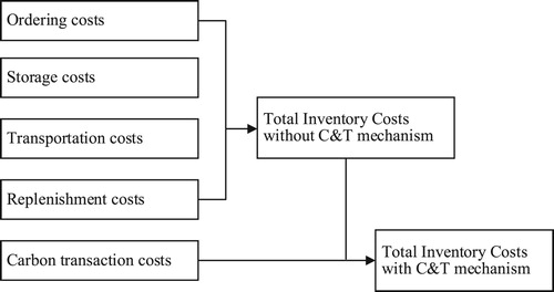
According to the characteristics of the demand for building materials and the hypothesis, the costs of ordering, storage, transportation, replenishment and carbon transaction are all included in the total inventory costs of building materials under the C&T mechanism. Clearly, the sum of the first four components is just the total inventory costs in the traditional model, as shown in Figure 1.

Figure 1. Composition of inventory costs.

This section focuses on the following. First, each cost component is explained, and the traditional $\left(s,S\right)$ model is constructed and solved. Then, the $\left(s^{\ast },S^{\ast }\right)$ model under the C&T mechanism is constructed and solved. Finally, several propositions are presented.

3.1. Cost components

There are $m$ possibilities for the demand of a certain type of building material per period. The values of $r$ can be taken as r₁, … , r_i, r_i+1, … , r_m, (r_i < r_i+1), and the corresponding probabilities are p(r₁) … , p(r_i), p(r_i+1), … , p(r _m), ${\sum }_{i=1}^{m}p\left(r_i\right)=1$. The initial inventory and order quantity are $I$ and $Q$, respectively, and the maximum inventory is $S=I+Q$. The various costs considered in each period are as follows:

3.1.1. Ordering costs

Because $r$ is a discrete random variable within the period, the corresponding ordering costs have two possible cases:

1. When $r\le I+Q$, ordering (order quantity: $Q$) occurs only once within the period, and the ordering costs are $c_1+c_{2}Q$.

2. When $r>I+Q$, in addition to ordering (order quantity: $Q$) once at the beginning of the period, emergency replenishment (replenishment quantity: $r-(I+Q)$) occurs. The total purchase quantity is $r-I$, and the ordering costs are $\left[c_1+c_2(r-I)\right]$.

Thus, the necessary ordering costs during the period are (1) $C_1=\sum _{r\le I+Q}(c_1+c_{2}Q\left)p\right(r)+\sum _{r>I+Q}\left[c_1+c_2(r-I)\right]p(r)$(1)

3.1.2. Storage costs

As $r$ is a discrete random variable within a period, the average storage quantity has two possible cases:

1. When $r\le I+Q$, the inventory is $I+Q$ and $I+Q-r$ at the beginning and end of the period, respectively, the average inventory is $I+Q-\left(r/2\right)$, and the storage costs are $c_3\left(I+Q-\left(r/2\right)\right)$.

2. When $r>I+Q$, the inventory is $I+Q$ and 0 at the beginning and end of the period, respectively, and $r-(I+Q)$ units of products are replenished during the period. The average inventory is $r/2$, and the storage costs are $c_3\left(r/2\right)$.

Thus, the necessary storage costs during the period are (2) $C_2=\sum _{r\le I+Q}{c}_3\left(I+Q-\frac{r}{2}\right)p\left(r\right)+\sum _{r>I+Q}{c}_3\frac{r}{2}p\left(r\right)$(2)

3.1.3. Transportation costs

As $r$ is a discrete random variable within a period, transportation costs are also calculated for two possible cases.

1. When $r\le I+Q$, $Q$ units of products are purchased during the period, and the transportation costs are $c_{4}Q$.

2. When $r>I+Q$, $r-I$ units of products are purchased during the period, and the transportation costs are $c_4(r-I)$.

Thus, the necessary transportation costs during a period are (3) $C_3=\sum _{r\le I+Q}{c}_{4}Qp\left(r\right)+\sum _{r>I+Q}{c}_4(r-I)p\left(r\right)$(3)

3.1.4. Replenishment costs

When $r>I+Q$, the replenishment quantity is $r-(I+Q)$, and the necessary replenishment costs during the period are (4) $C_4=\sum _{r>I+Q}{c}_5\left[r-(I+Q)\right]p\left(r\right)$(4)

3.1.5. Carbon Transaction costs

The carbon emissions in the period consist of two components, emissions produced by product transportation and storage. The assumptions are consistent with those of Hua et al. (2011), Hovelaque and Bironneau (2015), Liao and Deng (2018).

1. Expected carbon emissions from transportation

The carbon emissions from transportation include a fixed component and a variable component associated with the quantity of product purchased during the period. When $r\le I+Q$, $Q$ units of product are ordered; when $r>I+Q$, $r-I$units of product are purchased. Therefore, the total expected carbon emissions from transportation during the period are (5) $E_1=\sum _{r\le I+Q}(e_0+eQ\left)p\right(r)+\sum _{r>I+Q}[e_0+e(r-I\left)\right]p\left(r\right)$(5)

• (ii) Expected carbon emissions from storage

The carbon emissions from storage include a fixed part and a variable part related to the average inventory during the period. When $r\le I+Q$, the average inventory is $I+Q-\left(r/2\right)$; when $r>I+Q$, the average inventory is $r/2$. Therefore, the expected carbon emissions from storage during the period are (6) $\begin{array}{r}{E}_2=\sum _{r\le I+Q}\text{[}{\text{g}}_{\text{0}}+\text{g}\left(I+Q-\frac{r}{2}\right)\left]p\right(r)+\sum _{r>I+Q}(g_0+g\frac{r}{2})p\left(r\right)\end{array}$(6) Equations (5) and (6) are integrated to obtain the total expected carbon emissions during the period, which are expressed as (7) $E\left(Q\right)=E_1+E_2$(7)

$A$ represents the carbon emissions quotas allocated to the construction enterprise for the transportation and storage of a certain type building material, and $C$ is the carbon price during the period; therefore, the carbon transaction costs are (8) $C_5=C\left[E\right(Q)-A]$(8)

3.2. The $\left(s,S\right)$ model and solution without the C&T mechanism

When the C&T mechanism is not considered, the expected total costs of building materials inventory during each period include the ordering, storage, transportation, and emergency replenishment costs. Equations (1–4) are integrated to establish the traditional inventory model: (9) $minTC\left(Q\right)=C_1+C_2+C_3+C_4$(9) By substituting $Q=S-I$ into Equation (9), we obtain (10) $\begin{array}{rl}minTC\left(S\right)& =\sum _{r\le S}\left[\right(c_2+c_3+c_4)S-c_3\frac{r}{2}\\ & -(c_2+c_4)I\left]p\right(r)+c_1\\ & +\sum _{r>S}[-c_{5}S+(c_2+\frac{c_3}{2}+c_4+c_5)r\\ & -(c_2+c_4)I\left]p\right(r)\end{array}$(10)

1. Solution of the economic order quantity $Q^0$ in each period

As $I$ is known constant at the beginning of each period, the economic order quantity $Q^0$ can be obtained by solving the optimal maximum inventory level $S^0$.

By means of operation optimization, Equation (11) can be derived, in terms of which $S_i$ is determined and $S_i$ is the optimal solution of Equation (10). (See Appendix for details of the calculation for $S^0$.) (11) $\sum _{r\le S_{i-1}}p\left(r\right)\le M\le \sum _{r\le S_i}p\left(r\right),M=\frac{c_5}{c_2+c_3+c_4+c_5}$(11) Let $S^0=S_i$. Because $TC\left(Q\right)=TC\left(S\right)$, $S^0$ for the minimization of $TC\left(S\right)$ corresponds to $Q^0=S^0-I$, namely, the economic order quantity in the traditional model $\left(s,S\right)$ for the construction enterprise.

• (ii) Solution of the order point $s$ at the beginning of each period

The other problem for the model is to determine the order point $s$ at the beginning of a period.

When $I\ge s$, ordering may not be performed.

When $I<s$, ordering is necessary, and the order quantity ($Q^0=S^0-I$) is required to increase the storage quantity to $S^0$.

When the initial inventory is assumed to be $s$ (i.e. no ordering at the moment), there are no order costs. In the case of a stockout within a period, a one-off replenishment of $r-s$ is performed, so the total inventory costs can be expressed as (12) $\begin{array}{rl}TC\left(s\right)& =\sum _{r\le s}\left[\right(c_2+c_3+c_4)s-\frac{c_3}{2}r]p\left(r\right)\\ & +\sum _{r>s}[-c_{5}s+(c_2+\frac{c_3}{2}+c_4+c_5)r\left]p\right(r)\end{array}$(12) When the initial inventory is less than $s$, ordering occurs with economic order quantity $Q^0$ to ensure the initial maximum inventory is $S^0$, and the total inventory costs are (13) $\begin{array}{rl}TC\left(S^0\right)& =\sum _{r\le S^0}\left[\right(c_2+c_3+c_4)S^0-\frac{c_3}{2}r\left]p\right(r)\\ & +\sum _{r>S^0}[-c_5{S}^0+(c_2+\frac{c_3}{2}+c_4+c_5)r\left]p\right(r)+c_1\end{array}$(13)

Let $TC\left(s\right)\le TC\left(S^0\right)$; then, (14) $\begin{array}{rl}& \sum _{r\le s}\left[\right(c_2+c_3+c_4)s-\frac{c_3}{2}r]p\left(r\right)\\ & +\sum _{r>s}[-c_{5}s+(c_2+\frac{c_3}{2}+c_4+c_5)r\left]p\right(r)\\ & \le \sum _{r\le S^0}\left[\right(c_2+c_3+c_4)S^0-\frac{c_3}{2}r\left]p\right(r)\\ & +\sum _{r>S^0}[-c_5{S}^0+(c_2+\frac{c_3}{2}+c_4+c_5)r\left]p\right(r)+c_1\end{array}$(14) The method for calculating $s$ is to find the minimum of $r_i(r_i\le S^0)$ that satisfies Inequality (14).

$S^0$ is obtained from r₁, … , r_i, r_i+I, … , r_m. When $s<S^0$, the value of the first part on the left side of Inequality (14) is less than that of the first part on the right side, but the value of the second part on the left side is greater than that of the second part on the right side. Moreover, one additional part ($c_1$) is included on the right side of Inequality (14). Thus, Inequality (14) still appears to be workable. In the worst case (i.e. $s=S^0$), the Inequality definitely has a solution. Derivation of the solution expression for $s$ is more complicated than that for $S^0$, but the calculation of the value of $s$ is not difficult for a specific problem, as will be presented in Section 4.

3.3. The $\left(s^{\ast },S^{\ast }\right)$ model and solution with the C&T mechanism

Under the C&T mechanism, the expected total costs of building materials inventory in each period include the ordering, storage, transportation, emergency replenishment and carbon transaction costs. Integrating Equation (8) with Equation (9), the $\left(s^{\ast },S^{\ast }\right)$ inventory model with the C&T mechanism is established as (15) $minTC(Q{)}_e=TC\left(Q\right)+C_5$(15) By inserting $Q=S-I$ into Equation (15), we obtain (16) $\begin{array}{rl}& minTC(S{)}_e\\ & =\sum _{r\le S}\left\{\right[(c_2+c_3+c_4+C(e+g\left)\right]S\\ & -\frac{c_3+Cg}{2}r+c_1-(c_2+c_4+Ce)I\}p\left(r\right)\\ & +\sum _{r>S}[-c_{5}S+(\frac{c_3+Cg}{2}+c_2+c_4+c_5+Ce)\\ & r+c_1-(c_2+c_4+Ce)I]p\left(r\right)\\ & -CA+C(e_0+g_0)\end{array}$(16)

Under the C&T mechanism, the calculation of $S^{\ast }$ in the $\left(s^{\ast },S^{\ast }\right)$ model can be implemented with reference to the calculation processes for determining S⁰. The expression for determining ${S_i}^{\ast }$, the optimal solution of Equation (16), can be derived as Equation (17). (17) $\begin{array}{rl}& \sum _{r\le S_{i-1}}p\left(r\right)\le N\le \sum _{r\le S_i}p\left(r\right),N\\ & =\frac{c_2}{c_1+c_2+c_4+k+C\cdot (e+g)}\end{array}$(17) Let $S^{\ast }={S_i}^{\ast }$; the economic order quantity within the period is $Q^{\ast }=S^{\ast }-I$.

The solution of the order point $s^{\ast }$ under the C&T mechanism can be obtained with reference to the calculation processes for determining $s$. An example of the calculation of $s^{\ast }$ will be presented in Section 4.

3.4. Discussion

Proposition 3.1: In most cases, the optimal economic order quantity under the C&T mechanism can reduce the carbon emissions from the transportation and storage of building materials with discrete stochastic demand.

Proof: When $C>0$, the accumulated probability $M$ for determining $S^0$ is necessarily more than the $N$ for determining $S^{\ast }$, namely, $c_2/\left(c_1+c_2+c_4+k\right)>c_2/\left(c_1+c_2+c_4+k+C(e+g)\right)$. Thus, $S^0>S^{\ast }$ is usually true. Because $Q=S-I$, the relationship $Q^{{}_0}>Q^{\ast }$ exists.

In addition, because $r_i$ is a discrete randomly distributed variable, $M-N\le {\sum }_{r\le s_{i+n}}p\left(r\right)-{\sum }_{r\le s_i}p\left(r\right)$, n = 1, 2, … , m may likely occur while $r_i$ is sufficiently centrally distributed; that is, the difference between $M$ and $N$ is so small that it is unlikely to change the maximum inventory quantity, and $S^0=S^{\ast }$ may occur. Thus, $Q^{{}_0}=Q^{\ast }$ may naturally exist.

Therefore, when $C>0$, we obtain $Q^{{}_0}\ge Q^{\ast }$.

Moreover, Equations (5–7) indicate that for $E_1,E_2$ and $E\left(Q\right)$, because $E\left(Q\right)$ is an increasing function of $Q$, and when $C>0$ and $Q^{{}_0}\ge Q^{\ast }$, $E\left(Q^{\ast }\right)\le E\left(Q^0\right)$may naturally exist. Thus, the carbon emissions from the transportation and storage of building materials corresponding to $Q^{\ast }$under the C&T mechanism are generally less than those corresponding to Q⁰ without the C&T mechanism.

Proposition 3.2: Under the C&T mechanism, the optimal economic order quantity and expected carbon emissions are not related to the carbon quotas (caps) allocated to the enterprise by the government but have a reverse relationship with the carbon trading price.

Proof: Equation (17) for determining $S^{\ast }$ shows that the value of $S^{\ast }$ is not related to $A$ but has a reverse relationship with the carbon price $C$, namely, $S^{\ast }$ decreases as carbon price increases, and vice versa. In addition, because $E\left(Q^{\ast }\right)$ is an increasing function of $Q^{\ast }$, $E\left(Q^{\ast }\right)$ decreases as carbon price increases, and vice versa, and is not related to $A$.

Therefore, the optimal economic order quantity and expected carbon emissions are not related to carbon caps but have an inverse relationship with carbon price.

Proposition 3.3: A strict C&T mechanism will increase the total inventory costs while promoting emissions reduction. A moderate C&T mechanism can achieve a win-win result of emissions reduction and costs saving. However, a weak C&T mechanism is often ineffective in reducing carbon emissions but may benefit the construction enterprises.

Proof:

1. Under the C&T mechanism, when ordering building materials with $Q^{\ast }$

The formula $TC(Q^{\ast }{)}_e=TC\left(Q^{\ast }\right)+C\left[E\right(Q^{\ast })-A]$ can be rewritten as $TC(Q^{\ast }{)}_e-TC\left(Q^0\right)=TC\left(Q^{\ast }\right)+C\left[E\right(Q^{\ast })-A]-TC\left(Q^0\right)$When $TC(Q^{\ast }{)}_e-TC\left(Q^0\right)=0$, we have $A=\left(TC\left(Q^{\ast }\right)-TC\left(Q^0\right)\right)/C+E\left(Q^{\ast }\right)$.

Let (18) $\overline{A}=\frac{TC\left(Q^{\ast }\right)-TC\left(Q^0\right)}{C}+E\left(Q^{\ast }\right)$(18) And the following relationships exist: for $A<\overline{A}$, there is $TC(Q^{\ast }{)}_e>TC\left(Q^0\right)$; for $A=\overline{A}$, there is $TC(Q^{\ast }{)}_e=TC\left(Q^0\right)$; and for $A>\overline{A}$, there is $TC(Q^{\ast }{)}_e<TC\left(Q^0\right)$.

• (ii) Under the C&T mechanism, when ordering the building materials with $Q^0$,

The formula $TC(Q^0{)}_e=TC\left(Q^0\right)+C\left[E\right(Q^0)-A]$ can be rewritten as $TC(Q^0{)}_e-TC\left(Q^0\right)=C\left[E\right(Q^0)-A]$When $TC(Q^0{)}_e-TC\left(Q^0\right)=0$, we have A = E(Q⁰).

And the following relationships exist: when $A<E\left(Q^0\right)$, there is $TC(Q^0{)}_e>TC\left(Q^0\right)$; when $A=E\left(Q^0\right)$, there is $TC(Q^0{)}_e=TC\left(Q^0\right)$; and when $A>E\left(Q^0\right)$, there is $TC(Q^0{)}_e<TC\left(Q^0\right)$.

According to Proposition 3.1, when $C>0$, the relationship E(Q*) ≤ E(Q⁰) naturally exists. In combination with the above proofing process, the following results are obtained.

For each carbon price $C$, there is a carbon cap threshold $\overline{A}$. When $A<\overline{A}$, which can be seen as a strict C&T mechanism, the relationship $TC(Q^{\ast }{)}_e>TC\left(Q^0\right)$ exists. Namely, the strict C&T mechanism can urge construction enterprises to reduce emissions but will increase the total costs of inventory for building materials.

For each carbon price $C$, when $\overline{A}<A<E\left(Q^0\right)$, which can be seen as a moderate C&T mechanism, the relationship $TC(Q^{\ast }{)}_e<TC\left(Q^0\right)$ exists. Namely, the moderate C&T mechanism will not only encourage construction enterprises to reduce carbon emissions but also reduce total inventory costs, which will help to achieve economic benefits for enterprises and social benefits of emissions reduction, a win-win result.

For each carbon price $C$, when $A>E\left(Q^0\right)$, which can be seen as a weak C&T mechanism, the relationship $TC(Q^0{)}_e<TC\left(Q^0\right)$ exists. Namely, the weak C&T mechanism will not promote emissions reduction but will benefit the construction enterprises from the sale of carbon quotas.

4. Numerical verification

In this section, the optimal economic order quantities in the inventory models with and without the C&T mechanism are solved in MATLAB Software, and Propositions 3.1, 3.2 and 3.3 are validated. For this purpose, the parameter values are listed in Tables 2 and 3.

Table 2. Probability distributions of the demand for steel bars within a period.

$r_i\left(T\right)$	100	200	300	400	500	600	700	800	900	1000
$P\left(r_i\right)$	0.02	0.02	0.06	0.05	0.06	0.11	0.25	0.14	0.16	0.13
$\sum P\left(r_i\right)$	0.02	0.04	0.10	0.15	0.21	0.32	0.57	0.71	0.87	1.00

Table 3. Lists of various parameters.

Parameter	Value	Dimensions	Parameter	Value	Dimensions
$c_1$	500	$CNY/period$	$I$	80	$T$
$c_2$	210	$CNY/T$	$e_0$	30	$C{O}_{2}e/period$
$c_3$	8	$CNY/T$	$e$	2.4	$C{O}_{2}e/T$
$c_4$	40	$CNY/T$	$g_0$	15	$C{O}_{2}e/period$
$c_5$	50	$CNY/T$	$g$	0.6	$C{O}_{2}e/T$

The quantity and corresponding probability distributions of the demanded building materials of a construction enterprise are obtained by investigating the Engineering Department of a real estate company, and appropriate adjustments are made in accordance with the goal of this study. Table 2 lists the possible probabilities of demand for steel bars within an ordering period of a construction enterprise.

4.1. Verification of Propositions 3.1 and 3.2

The parameter values are integrated into Equation (11), and $M=0.1678$ is obtained. According to Table 2, $S^0=500$ corresponds to $Q^0=420$ (namely, the economic order quantity is 420 T of steel bars without the C&T mechanism); according to Equation (7), $E\left(Q^0\right)=1838.7C{O}_{2}es$.

When $C>0$, as the carbon price increases from $10CNY/C{O}_{2}e$ by a step of 10, we obtain various optimal economic order quantities of steel bars from Equation (17) and expected carbon emissions from Equation (7), as shown in Table 4.

Table 4. Optimal ordering quantities and expected emissions under the C&T mechanism.

$C\left(CNY/C{O}_{2}e\right)$	10	20–60	70–310	320–730	740 –
$S^{\ast }\left(T\right)$	500	400	300	200	100
$Q^{\ast }\left(T\right)$	420	320	220	120	20
$E\left(Q^{\ast }\right)\left(C{O}_{2}e\right)$	1838.7	1793.7	1763.7	1751.7	1745.7

Table 4 indicates that

• When $C=10$, $Q^{\ast }=420$;

• When $C\in [20,60]$, $Q^{\ast }=320$;

• When $C\in [70,310]$, $Q^{\ast }=220$;

• When $C\in [320,730]$, $Q^{\ast }=120$; and

• When $C\ge 740$,$Q^{\ast }=20$.

The last case represents the economic order quantity when the carbon emissions are at the minimum, which means carbon emissions cannot be reduced consistently by adjusting the order batch size, as shown in Figure 2.

Figure 2. Effects of carbon prices on EOQ and carbon emissions.

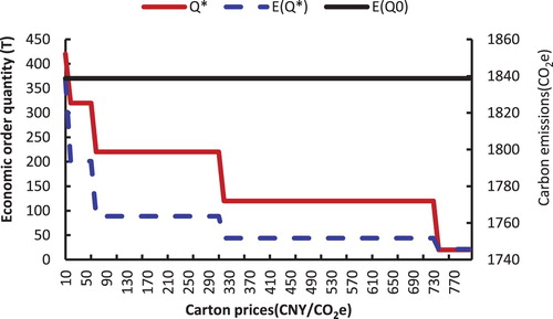
Figure 2 indicates that, under the C&T mechanism, when the construction enterprise purchases steel bars in economic order quantity with the lowest total costs, including carbon transaction costs, in most cases, carbon emissions from the inventory process will be reduced. The results show that the C&T mechanism is effective in reducing carbon emissions from building materials transportation and storage. Moreover, with an increase in carbon price, the optimal economic order quantity and the expected carbon emissions amount decrease, which shows that they have an inverse relationship with carbon price. Because the calculation of the optimal economic order quantities and carbon emissions does not involve the carbon cap, these factors are not related.

4.2. Verification of Proposition 3.3

When the carbon price varies in $C\in [10,100]$, the values of $\overline{A}$ can be obtained by Equation (18), as shown in Table 5.

Table 5. Carbon cap thresholds corresponding to carbon prices.

$C/\left(CNY/C{O}_{2}e\right)$	10	20	30	40	50	60	70	80	90	100
$\overline{A}/C{O}_{2}e$	1838.7	1820.2	1811.4	1807.0	1804.3	1802.5	1800.1	1795.6	1792.0	1789.2

For example, when $C=20CNY/C{O}_{2}e$ and $\overline{A}=\text{1820}\text{.2}C{O}_{2}es$, $TC(Q^{\ast }{)}_e$ can be obtained by Equation (15) for various values of $A$. $E\left(Q^0\right)=1838.7C{O}_{2}es$ is known, and the values of $TC\left(Q^0\right)$and $TC(Q^0{)}_e$can be calculated, as shown in Table 6.

Table 6. The effects of carbon caps on expected total costs.

$A/C{O}_{2}e$	$TC(Q^{\ast }{)}_e/CNY$	$TC(Q^0{)}_e/CNY$	$TC\left(Q^0\right)/CNY$
1800	172036	172406	171632
1805	171936	172306	171632
1810	171836	172206	171632
1815	171736	172106	171632
1820.2	171632	172002	171632
1825	171536	171906	171632
1830	171436	171806	171632
1835	171336	171706	171632
1838.7	171262	171632	171632
1840	171236	171606	171632
1845	171136	171506	171632
1850	171036	171406	171632
1855	170936	171306	171632

Figure 3 is based on Table 6.

Figure 3. Comparison of the effects of different C&T mechanisms.

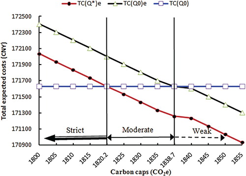
According to the above discussion, when $C=20CNY/C{O}_{2}e$, the carbon cap threshold $\overline{A}=\text{1820}\text{.2}C{O}_{2}es$, $E\left(Q^{\ast }\right)=1793.7C{O}_{2}es$, and $E\left(Q^0\right)=1838.7C{O}_{2}es$.

4.3. Verification of the effects of different C&T mechanisms on emissions reduction

1. The effects of the strict C&T mechanism

As shown in Figure 3, when $C=20CNY/C{O}_{2}e$ and $A<1820.2C{O}_{2}es$, the C&T mechanism is strict, corresponding to the left side of the $\overline{A}$ vertical line. In this case, $E\left(Q^{\ast }\right)\le E\left(Q^0\right)$ and $TC\left(Q^0\right)<TC(Q^{\ast }{)}_e$, which indicates that the strict C&T mechanism encourages firms to reduce emissions by adjusting order quantity but simultaneously increases total inventory costs.

• (ii) The effects of the moderate C&T mechanism

As shown in Figure 3, when $C=20CNY/C{O}_{2}e$ and $1820.2<A<1838.7C{O}_{2}es$, the C&T mechanism is moderate, corresponding to the middle part of the vertical lines of $\overline{A}$ and $E\left(Q_0\right)$. In this case, $E\left(Q^{\ast }\right)\le E\left(Q^0\right)$ and $TC(Q^{\ast }{)}_e<TC\left(Q^0\right)$, which indicates that a moderate C&T mechanism promotes emissions reductions while simultaneously reducing total inventory costs. The policy effect of emissions reduction and costs saving is win-win.

• (iii) The effects of the weak C&T mechanism

As seen in Figure 3, when $C=20CNY/C{O}_{2}e$ and $A>1838.7C{O}_{2}es$, the C&T mechanism is weak, corresponding to the right side of the vertical line of $E\left(Q_0\right)$. In this case, $TC(Q^0{)}_e<TC\left(Q^0\right)$, which indicates that, under the weak C&T mechanism, even if the enterprises do not reduce carbon emissions, they can still cut total inventory costs by selling extra carbon emissions quotas. Therefore, the weak C&T mechanism does very little to promote emissions reduction.

4.4. Calculation of order points

1. The order point $s$ in the $\left(s,S\right)$ model without the C&T mechanism

When the C&T mechanism is not considered, the optimal initial inventory maximum of steel bars in each period is $500Ts$ and $r_i$ may be $100,200,\text{ }300,\text{ }400\text{ or }500$. When $S^0=500$, the values of $TC\left(s\right)$ can be obtained by Equation (12), and the value of $TC\left(S^0\right)$ can be obtained by Equation (13). The results are shown in Table 7. Inequality (14) is true only when $s=500$; thus, the initial order point is $s=500$ in the traditional $\left(s,\text{ }S\right)$ model.

• (ii) The order point $s^{\ast }$ in the $\left(s^{\ast },\text{ }{S}^{\ast }\right)$ model with the C&T mechanism

Table 7. Determination of $s$ in the traditional $\left(s,S\right)$ model.

$r_i/T$	100	200	300	400	500
$TC\left(s\right)/CNY$	201094	196690	192882	190862	190332
$TC\left(S^0\right)/CNY$	——	——	——	——	190832

A similar calculation process can be utilized to determine the order point under the C&T mechanism. The values of the order point $s^{\ast }$ corresponding to various carbon prices are calculated based on the data of the example above, and the results are shown in Table 8.

Table 8. The $\left(s^{\ast },S^{\ast }\right)$ inventory arrangement with the C&T mechanism.

$C\left(CNY/T\right)$	$S^{\ast }\left(T\right)$	$s^{\ast }\left(T\right)$
10	500	400
[20-50]	400	400
60	400	300
[70-270]	300	300
[280-310]	300	200
[320-640]	200	200
[650-730]	200	100
740-	100	100

Comparison of the order points and maximum inventory levels for the procurement of steel bars shows that the initial order points under the C&T mechanism are not higher than those in the traditional model $\left(s,S\right)$. This result holds even if the carbon price is very low and the maximum inventories are equal in both models. Moreover, the order point under the C&T mechanism may gradually decrease with increasing carbon price.

5. Conclusions and future prospects

In this paper, the problem of inventory decision of a single type of building material under the dual constraints of the C&T mechanism and stochastic demand has been investigated. Two inventory models with and without the C&T mechanism have been constructed, and three Propositions have been proven. The optimal inventory arrangements have been obtained in the simulation section, and several interesting conclusions are reached, as follows:

1. For discrete and stochastic product demand, the optimal inventory arrangement under the C&T mechanism can reduce the carbon emissions from inventory processes. Similar results have been found in studies on deterministic demands. This result suggests that under any demand situation, enterprises can reduce the carbon emissions of inventory process by adopting the economic order quantity under the C&T mechanism.

2. Under the C&T mechanism, in most cases, the optimal economic order quantity and the expected carbon emissions from building materials inventory will decrease as the carbon price increases, and vice versa. However, the optimal economic order quantity is not related to the carbon cap, which suggests that policy-makers can force construction enterprises to reduce carbon emissions resulting from building material inventory processes by increasing the carbon trading price.

3. The strict C&T mechanism increases the total inventory costs while promoting emissions reduction; the moderate C&T mechanism achieves a win-win effect of carbon emissions reduction and inventory costs saving; and the weak C&T mechanism does little to reduce emissions and allows enterprises to benefit without reducing emissions.

4. The different effects of the C&T mechanism on each enterprise can be quantified according to various carbon trading prices and the basic emissions data, which provides a basis for policy-makers to allocate carbon quotas to enterprises and avoids the blindness in setting up the C&T mechanism.

Although some uncertainties of realistic demands for building materials have been considered in this study, many of the assumptions still have limitations, and the effects of those factors, such as delayed delivery, transportation routes, means of transportation, and constraints of warehousing volume at the construction sites, on ordering decisions have not been taking into account. In addition, the inventory decisions of multiple products for construction enterprises under the C&T mechanism have not been studied. These issues are worthy of further investigation.

Acknowledgements

The authors appreciate the reviewers and look forward to receiving their comments. If you have any queries, please do not hesitate to contact me.

Disclosure statement

No potential conflict of interest was reported by the authors.

Additional information

Funding

This research was supported by the National Science Foundation of China [grant number 51379171].

Appendix. Solution of the optimal initial inventory maximum $S^0$

The total inventory costs can be expressed as (A1) $\begin{array}{rl}minTC\left(S\right)& =\sum _{r\le S}\left[\right(c_2+c_3+c_4)S-c_3\frac{r}{2}-(c_2+c_4)I\left]p\right(r)+c_1\\ & +\sum _{r>S}[-c_{5}S+(c_2+\frac{c_3}{2}+c_4+c_5)\\ & r-(c_2+c_4)I\left]p\right(r)\end{array}$(A1) By substituting $S_{i+1}$, $S_i$ and $S_{i-1}$ into Equation (A1), we obtain (A2) $\begin{array}{rl}TC\left(S_{i+1}\right)& =\sum _{r\le S_{i+1}}\left[\right(c_2+c_3+c_4)S_{i+1}\\ & -c_3\frac{r}{2}-(c_2+c_4)I\left]p\right(r)+c_1\\ & +\sum _{r>S_{i+1}}[-c_5{S}_{i+1}+(c_2+\frac{c_3}{2}+c_4+c_5)\\ & r-(c_2+c_4)I\left]p\right(r)\end{array}$(A2) (A3) $\begin{array}{rl}TC\left(S_i\right)& =\sum _{r\le S_i}\left[\right(c_2+c_3+c_4)S_i-c_3\frac{r}{2}-(c_2+c_4)I\left]p\right(r)+c_1\\ & +\sum _{r>S_i}[-c_5{S}_i+(c_2+\frac{c_3}{2}+c_4+c_5)r-(c_2+c_4\left)I\right]p\left(r\right)\end{array}$(A3) and (A4) $\begin{array}{rl}TC\left(S_{i-1}\right)& =\sum _{r\le S_{i-1}}\left[\right(c_2+c_3+c_4)S_{i-1}\\ & -c_3\frac{r}{2}-(c_2+c_4)I\left]p\right(r)+c_1\\ & +\sum _{r>S_{i-1}}[-c_5{S}_{i-1}+(c_2+\frac{c_3}{2}+c_4+c_5)r\\ & -(c_2+c_4)I\left]p\right(r)\end{array}$(A4)

$r$ is sorted from small to large as r₁, … , r_i, r_i+1, … , r_m, (r_i < r_i+1).

Let $\mathrm{\Delta }{r}_i=r_{i+1}-r_i\ne 0(i=1,\cdots ,m)$.

$S$ is assigned a value in r₁, … , r_i, r_i+1, … , r_m. When S = r_i, it is written as S_i.

Let ΔS = S_i+1−S_i = r_i+1−r_i = Δr≠0 (i = 1, … , m).

$TC\left(S_i\right)$ is minimized to obtain the $S_i$ that conforms to the following inequalities: (A5) $TC\left(S_{i+1}\right)-TC\left(S_i\right)\ge 0$(A5) (A6) $TC\left(S_i\right)-TC\left(S_{i-1}\right)\le 0$(A6)

Let $\mathrm{\Delta }TC\left(S_i\right)=TC\left({S_i}_{+1}\right)-TC\left(S_i\right)$ and $\mathrm{\Delta }TC\left({S_i}_{-1}\right)=TC\left(S_i\right)-TC\left({S_i}_{-1}\right)$; Inequality (A5) can be written as (A7) $\mathrm{\Delta }TC\left(S_i\right)=\left[\right(c_2+c_3+c_4+c_5)\sum _{r\le S_i}p\left(r\right)-c_5]\cdot \mathrm{\Delta }{S}_i\ge 0$(A7) Because $\mathrm{\Delta }{S}_i\ne 0$, namely, $(c_2+c_3+c_4+c_5)\sum _{r\le S_i}p\left(r\right)-c_5\ge 0$, Inequality (A5) can be written as (A8) $\sum _{r\le S_i}p\left(r\right)\ge \frac{c_5}{c_2+c_3+c_4+c_5}$(A8)

Similarly, Inequality (A6) can be written as (A9) $\sum _{r\le S_{i-1}}p\left(r\right)\le \frac{c_5}{c_2+c_3+c_4+c_5}$(A9) Let $M=c_5/\left(c_2+c_3+c_4+c_5\right)$

Equations (A8) and (A9) can be integrated to obtain the expression for $S_i$ that minimizes $TC\left(S_i\right)$: (A10) $\sum _{r\le S_{i-1}}p\left(r\right)\le M\le \sum _{r\le S_i}p\left(r\right)$(A10) Let $S^0=S_i$; we then obtain the optimal maximum inventory at the beginning of the period.

References

- Bai, Q., Gong, Y., Jin, M., & Xu, X. (2019). Effects of carbon emission reduction on supply chain coordination with vendor-managed deteriorating product inventory. International Journal of Production Economics, 208, 83–99. doi: 10.1016/j.ijpe.2018.11.008
- Bonney, M., & Jaber, M. Y. (2011). Environmentally responsible inventory models: Non-classical models for a non-classical era. International Journal of Production Economics, 133(1), 43–53. doi: 10.1016/j.ijpe.2009.10.033
- Chen, X., Benjaafar, S., & Elomri, A. (2013). The carbon-constrained EOQ. Operations Research Letters, 41(2), 172–179. doi: 10.1016/j.orl.2012.12.003
- García-Alvarado, M., Paquet, M., Chaabane, A., & Amodeo, L. (2017). Inventory management under joint product recovery and cap-and-trade constraints. Journal of Cleaner Production, 167, 1499–1517. doi: 10.1016/j.jclepro.2016.10.074
- Ghosh, A., Jha, J. K., & Sarmah, S. P. (2017). Optimal lot-sizing under strict carbon cap policy considering stochastic demand. Applied Mathematical Modelling, 44, 688–704. doi: 10.1016/j.apm.2017.02.037
- Govindan, K., Azevedo, S. G., Carvalho, H., & Cruz-Machado, V. (2014). Impact of supply chain management practices on sustainability. Journal of Cleaner Production, 85, 212–225. doi: 10.1016/j.jclepro.2014.05.068
- Gui, Y., Shen, J., Hu, H., & Liu, Z. (2015). Research on model of stochastic inventory control under carbon emission trading mechanism. Journal of Shandong University(Natural Science), 50(9), 55–60.
- Hovelaque, V., & Bironneau, L. (2015). The carbon-constrained EOQ model with carbon emission dependent demand. International Journal of Production Economics, 164, 285–291. doi: 10.1016/j.ijpe.2014.11.022
- Hua, G., Cheng, T. C. E., & Wang, S. (2011). Managing carbon footprints in inventory management. International Journal of Production Economics, 132(2), 178–185. doi: 10.1016/j.ijpe.2011.03.024
- Huisingh, D., Zhang, Z., Moore, J. C., Qiao, Q., & Li, Q. (2015). Recent advances in carbon emissions reduction: Policies, technologies, monitoring, assessment and modeling. Journal of Cleaner Production, 103, 1–12. doi: 10.1016/j.jclepro.2015.04.098
- Lan, H., & Ji, S. (2013). Manufacturers’ ordering strategy under cap-and-trade mechanism. Systems Engineering, 31(12), 81–86.
- Li, G., & Zhang, C. (2015). Inventory management with carbon-constrained. Logistics Engineering and Management, 3, 68–72.
- Liao, H., & Deng, Q. (2018). A carbon-constrained EOQ model with uncertain demand for remanufactured products. Journal of Cleaner Production, 199, 334–347. doi: 10.1016/j.jclepro.2018.07.108
- Ma, C. S., Chen, X., Luo, Z. Y., & Li, T. (2015). Production strategy of considering low carbon emission policies regulation under stochastic demand. Control & Decision, 30(6), 969–976.
- Mukhopadhyay, A., & Goswami, A. (2014). Economic production quantity models for imperfect items with pollution costs. Systems Science & Control Engineering, 2(1), 368–378. doi: 10.1080/21642583.2014.912571
- Plambeck, E. L. (2012). Reducing greenhouse gas emissions through operations and supply chain management. Energy Economics, 34(3), S64–S74. doi: 10.1016/j.eneco.2012.08.031
- Purohit, A. K., Shankar, R., Dey, P. K., & Choudhary, A. (2016). Non-stationary stochastic inventory lot-sizing with emission and service level constraints in a carbon cap-and-trade system. Journal of Cleaner Production, 113(1), 654–661. doi: 10.1016/j.jclepro.2015.11.004
- Qu, X., Li, B., & Liu, X. (2015). Optimization research of supply chain considering defective-rate items under the carbon cap-and-trade mechanism. Management Review, 27(9), 187–200.
- Shankar, R. (2015). The value of VMI beyond information sharing under time-varying stochastic demand. International Journal of Production Research, 53(5), 1472–1486. doi: 10.1080/00207543.2014.951093
- Song, J., & Leng, M. (2012). Analysis of the single-period problem under carbon emissions policies. (Vol. 176, pp. 297–313). New York, NY: Springer.
- Stavins, R. N. (1999). Experience with market-based environmental policy instruments. Social Science Electronic Publishing, 1(03), 355–435.
- Tietenberg, T. (2003). The tradable-permits approach to protecting the commons: Lessons for climate change. Oxford Review of Economic Policy, 19(3), 400–419. doi: 10.1093/oxrep/19.3.400
- Toptal, A., Özlü, H., & Konur, D. (2014). Joint decisions on inventory replenishment and emission reduction investment under different emission regulations. International Journal of Production Research, 52(1), 243–269. doi: 10.1080/00207543.2013.836615
- Xu, J., Chen, Y., & Bai, Q. (2016). A two-echelon sustainable supply chain coordination under cap-and-trade regulation. Journal of Cleaner Production, 135, 42–56. doi: 10.1016/j.jclepro.2016.06.047
- Xu, X., Zhang, W., He, P., & Xu, X. (2017). Procudion and pricing problems in make-to-order supply chain with cap-and-trade regulation. Omega, 66, 248–257. doi: 10.1016/j.omega.2015.08.006
- Yenipazarli, A. (2016). Managing new and remanufactured products to mitigate environmental damage under emissions regulation. European Journal of Operational Research, 249(1), 117–130. doi: 10.1016/j.ejor.2015.08.020
- Yue, X., & Guo, J. (2015). Carbon emission management under low-carbon perspective: An empirical study based on engineering cost. Project Management Technology, 13(2), 67–71.