Integration of fault diagnosis and control based on residual decoupling

Abstract

In this paper, an integrated framework for fault diagnosis and control is designed based on residual decoupling technology, which has fully considered the balance between the robustness of control system and the sensitivity of fault diagnosis system. To this end, the decoupling technology is first used for separation of fault and disturbance. Then, robust controller and fault-tolerant controller are designed for rejecting the system disturbance and guaranteeing the system performance, respectively. Finally, the application to three-tank system is given to demonstrate the performance and effectiveness of the proposed methods.

Keywords:

• Integration of fault diagnosis and control
• residual decoupling
• fault-tolerant control
• fault diagnosis

1. Introduction

Associated with the increasing demands on large-scale, continuous, high-speed and high-quality for modern industrial production, fault diagnosis and control have received considerable attention in both research and industrial application domains, and a large number of fault diagnosis and control methods have been developed (Ding, 2013, 2014; Lan & Patton, 2018; Li, Wang, Wang, & Alsaadi, 2017; Li, Luo, Ding, Yang, & Peng, 2019; Shen, Ding, & Wang, 2013; Xiang, Li, & Zhang, 2018; Yin, Wang, & Yang, 2014). The existing fault diagnosis methods, however, generally do not take into account the balance between the robustness of control system and the sensitivity of fault diagnosis system, which may affect the performance of fault diagnosis system. Accordingly, in order to meet the requirements of product quality and safety production in complex industrial processes, it is necessary to promote integrated design and research of automatic control system for industrial process control and fault diagnosis (Lan & Patton, 2018; Xiang et al., 2018).

In the industrial process, the abnormal behaviour is generally defined as a fault, which is an unpermitted deviation of at least one characteristic property of the system from the acceptable, usual, standard condition (Isermann, 2006; Yin et al., 2014). When the fault is not serious, the robust control and active fault-tolerant control methods can be used to suppress the effects of disturbance, noise or minor failures on the system. For these purposes, a residual generation method was proposed for fault diagnosis in the presence of disturbances (Gertler & Kunwer, 1995). Under this framework, Zhang, Marios, and Thomas (2002) developed a robust detection and isolation method for abrupt and incipient faults in nonlinear systems. Zhang and Jiang (2001) put forward an integrated fault detection, diagnosis and reconfigurable control scheme based on interacting multiple model (IMM) approach. Paoli, Matteo, and Stéphane (2011) proposed an active fault-tolerant control method of discrete event systems using online diagnostics. Zhang, Yang, Ding, and Li (2016) proposed an optimal design method of residual-driven dynamic compensator based on iterative algorithms with guaranteed convergence. These representative robust control and active fault-tolerant control methods have promoted the development of process control theory and received enhanced attention.

The goal of fault diagnosis is not only to keep the plant operator and maintenance personnel better informed of the state of the process, but also to assist them to make appropriate remedial actions to remove the abnormal behaviour from the process. For these purposes, model-based fault diagnosis methods act as basic tools to design and carry out some monitoring activities (Ding, 2013; Isermann, 2006; Tidriri, Chatti, Verron, & Tiplica, 2016), which are suitable for deep understanding of the plant, i.e. the accurate analytic model can be established and the residual signal can be constructed by observing the input and output data. In comparison, data-based methods, thanks to their simple forms and fewer requirements on the design and engineering efforts, have become more and more popular nowadays (Ding, 2014; Ge, Song, & Gao, 2013; Ma, Dong, Peng, & Zhang, 2019; Yin et al., 2014). However, most of the model-based and data-based fault diagnosis methods are separately studied from process control, which may result in time delay and nonrobustness to external disturbance.

Strongly motivated by those observations, in this paper, we hope to achieve an integrated design scheme, where the balance between the robustness of control system and the sensitivity of fault diagnosis system has been fully considered. To be specific, the main contributions are:

• to propose an integrated framework for fault diagnosis and control based on residual decoupling technology;

• to put forward a separation method of fault and disturbance based on decoupling technology;

• to develop new robust controller and fault-tolerant controller design methods for rejecting the system disturbance and guaranteeing the system performance.

The remainder of this paper is organized as follows. In Section 2, the robustness and sensitivity for the fault diagnosis and control systems are discussed. Sections 3 concentrates on the integrated design scheme based on internal model control. Then, the verification results are presented in Section 4. In Section 5, concluding remarks and some outlooks are summarized.

2. Integrated design scheme based on internal model control

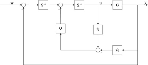
Generalized internal model control (GIMC) includes two parts: one part for performance and the other part for robustness (Zhou & Zhang, 2001). The part for robustness will be active when there are faults, which ensures that the system has good performance index without faults. When faults happen, the fault-tolerant control system has the ability to tolerate them. The structure of GIMC is shown in Figure 1. Where w is given parameter, u is controlled variable, y is output, G is the plant, Q is the robust controller, $\hat{\mathbf{N}}$, $\hat{\mathbf{M}}$, $\hat{\mathbf{Y}}$, ${\hat{\mathbf{X}}}^{-1}$ are the left coprime factors.

Figure 1. Schematic diagram of GIMC.

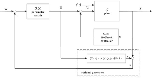
Extended internal model control (EIMC) can achieve integrated design of fault diagnosis and control based on the coprime decomposition and Youla parameterization theory, where embedded state observer and residual generator are built, and the indicator of $H_{\mathrm{\infty }}$ is used to assess residual to ensure good fault diagnosis performance (Ding, 2009). It also provides a very important reference value for fault diagnosis. EIMC structure is shown in Figure 2, where ${\mathbf{K}}_{\mathbf{1}}\mathbf{\left(}\mathbf{s}\mathbf{\right)}$ is the feedback controller, $\overline{\mathbf{r}}$ is the output of residual generator, ${\mathbf{Q}}_{\mathbf{2}}\mathbf{\left(}\mathbf{s}\mathbf{\right)}$ is a stable controller.

Figure 2. Schematic diagram of EIMC.

In GIMC, the control performance and robustness of the system are designed separately so that the system can maintain good states when there are no disturbances or faults. Meanwhile, when any faults or disturbances happen, the system can ensure safety by means of robust control. In contrast, the EIMC, as a result of the observer form of the Youla parameterization, all stabilizing controllers can be realized as an observer-based state feedback controller. From the viewpoint of the integrated design, it has the advantage of a direct access to the residual signals.

Based on GIMC, EIMC and the idea of residual decoupling and optimal controller design, an integrated design scheme based on residual decoupling is proposed, where the following aspects are mainly considered:

• uncertainty of the system, i.e. unknown disturbances or various types of faults.

• controller design, including stable controller, robust controller and fault-tolerant controller.

• fault diagnosis, where the design of residual generator and evaluation method need to be considered.

• integrated design and analysis, mainly aiming at the robustness and sensitivity of fault diagnosis.

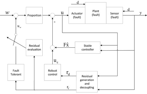
The schematic diagram of the integrated design is shown in Figure 3, where the plant includes equipments, actuators and sensors, the disturbances $\mathbf{d}$ are mainly presented in the equipments and the sensors, and faults may occur in every parts. The parameters in proportional component are fixed, and the stable controller is mainly designed by using state observer. The residual decoupling is used for residual generation and decoupling that are produced by the residual ${\mathbf{r}}_{\mathbf{d}}$ affected by disturbances and the residual ${\mathbf{r}}_{\mathbf{f}}$ affected by faults. The residual evaluation part performs switch operation between fault diagnosis and fault-tolerant. When there are no faults or disturbances, the stabilization controller is used for keeping the system working stably. When faults or disturbances happen, the system will deviate from its normal working state, and robust control and fault-tolerant will be performed.

Figure 3. Schematic diagram of the integrated design.

3. Integrated design method of fault diagnosis and control

3.1. Basic description

The structure of double closed-loop is used to realize the integrated design of fault diagnosis and control. Five parts are mainly included, namely, stable controller, residual generator, fault diagnosis, robust controller and fault-tolerant controller (Diversi & Simani, 2013; Zhang & Ding, 2007).

• Stable controller. State feedback based on observer is used to ensure the stability of the system, including the construction of state observer and the choice of state feedback matrix. The main purpose is to ensure that the system can work well in normal state and remain stable in the absence of disturbances and faults by means of feedback control.

• Residual generator. Parametric form of residual generator is derived from coprime decomposition and Youla parametric theories. Based on the idea of residual decoupling, the observation and post-filter matrixes are designed to build special residual generator to produce two residuals, ${\mathbf{r}}_{\mathbf{d}}$ and ${\mathbf{r}}_{\mathbf{f}}$, where ${\mathbf{r}}_{\mathbf{d}}$ is only related to the disturbance of the system, and ${\mathbf{r}}_{\mathbf{f}}$ is only related to the system fault.

• Fault diagnosis. ${\mathbf{r}}_{\mathbf{f}}$ is assessed according to relevant fault diagnosis methods, determining whether the fault occurs and fault-tolerant switch operates.

• Robust controller ${\mathbf{K}}_{\mathbf{1}}$. It is a dynamic controller. The optimal robust controller is designed by the establishment of LQ state regulator performance indicator. The input signal is ${\mathbf{r}}_{\mathbf{d}}$, and the output signal is ${\mathbf{u}}_{\mathbf{c}}$.

• Fault-tolerant controller ${\mathbf{K}}_{\mathbf{2}}$. It is a dynamic controller as well. LQ tracker performance indicator is adopted to design fault-tolerant controller. The input signal is ${\mathbf{r}}_{\mathbf{f}}$ and the output signal is ${\mathbf{u}}_{\mathbf{w}}$, which is essentially the feed-forward compensation for the fault. When the fault is diagnosed, the switch is closed. As a result, ${\mathbf{u}}_{\mathbf{w}}$ is added to the given parameters, and fault-tolerant control is carried out.

3.2. Residual generation and decoupling

The system is affected by the disturbance and the fault, the basic form of residual generator can be described by: (1) $\begin{array}{rl}\mathbf{r}\left(p\right)& =\mathbf{R}\left(p\right)\hat{\mathbf{M}}\left(p\right)\left({\mathbf{G}}_{yd}\left(p\right)\mathbf{d}\left(p\right)+{\mathbf{G}}_{yf}\left(p\right)\mathbf{f}\left(p\right)\right)\\ & =\mathbf{R}\left(p\right)\left({\hat{\mathbf{N}}}_d\left(p\right)\mathbf{d}\left(p\right)+{\hat{\mathbf{N}}}_f\left(p\right)\mathbf{f}\left(p\right)\right)\end{array}$(1) According to the basic derivation of the left coprime decomposition, the residuals can be analysed, and the basic forms are as follows: (2) $\begin{array}{rl}\mathbf{r}\left(p\right)& ={\mathbf{r}}_d\left(p\right)+{\mathbf{r}}_f\left(p\right)\end{array}$(2) (3) $\begin{array}{rl}{\mathbf{r}}_d\left(p\right)& =\mathbf{v}{\hat{\mathbf{N}}}_d\left(p\right)\mathbf{d}\left(p\right)=\mathbf{v}\mathbf{C}{\left(p\mathbf{I}-{\mathbf{A}}_L\right)}^{-1}{\mathbf{E}}_d\end{array}$(3) (4) $\begin{array}{rl}{\mathbf{r}}_f\left(p\right)& =\mathbf{v}{\hat{\mathbf{N}}}_f\left(p\right)\mathbf{f}\left(p\right)=\mathbf{v}\mathbf{C}{\left(p\mathbf{I}-{\mathbf{A}}_L\right)}^{-1}{\mathbf{E}}_f\end{array}$(4) where $\mathbf{r}\left(p\right)$ is the residual of the system, ${\mathbf{r}}_d\left(p\right)$ and ${\mathbf{r}}_f\left(p\right)$ are the parts of the residual due to the disturbance and fault, respectively, $\mathbf{v}$ is the the post-filter.

In practice, the disturbance and fault are coupled together. Accordingly, the residual decoupling should be performed. In the case of residual decoupling, the residual structure of the observer can be allocated according to the form of residual signal, combined with the design of post-filter to achieve complete decoupling of the residual for disturbance. Based on the same principle, we extend this method to the residual decoupling calculation of the fault.

The decoupling of residual can be described as two questions.

1. According to the feature structure assignment, observation matrix ${\mathbf{L}}_{\mathbf{f}}$ and filter matrix ${\mathbf{V}}_{\mathbf{2}}$ are designed to achieve the complete residual decoupling for disturbance. The residual ${\mathbf{r}}_f\left(p\right)$, which reflects the effect of the fault, is obtained and should meet the following conditions: (5) $\begin{array}{rl}{\mathbf{r}}_d\left(p\right)& ={\mathbf{V}}_2\mathbf{C}{\left(p\mathbf{I}-\mathbf{A}+{\mathbf{L}}_f\mathbf{C}\right)}^{-1}{\mathbf{E}}_d=0\end{array}$(5) (6) $\begin{array}{rl}{\mathbf{r}}_f\left(p\right)& ={\mathbf{V}}_2\mathbf{C}{\left(p\mathbf{I}-\mathbf{A}+{\mathbf{L}}_f\mathbf{C}\right)}^{-1}{\mathbf{E}}_f\ne 0\end{array}$(6)

   Given that observation matrix $\mathbf{A}-\mathbf{L}\mathbf{C}\in {\mathbf{R}}^{n\times n}$ can be diagonalized, with eigenvalues ${\lambda }_i,i=1,\dots ,n$, and its left and right eigenvectors are ${\mathit{\alpha }}_i\in {\mathbf{R}}^{1\times n},{\mathit{\beta }}_i\in {\mathbf{R}}^{n\times 1}$, which should satisfy Equation (5(5) $\begin{array}{rl}{\mathbf{r}}_d\left(p\right)& ={\mathbf{V}}_2\mathbf{C}{\left(p\mathbf{I}-\mathbf{A}+{\mathbf{L}}_f\mathbf{C}\right)}^{-1}{\mathbf{E}}_d=0\end{array}$(5) ). Observation matrix ${\mathbf{L}}_f$ and the filter matrix ${\mathbf{V}}_{\mathbf{2}}$ should be satisfied: (7) ${\mathbf{V}}_2\mathbf{C}{\mathit{\beta }}_1{\mathit{\alpha }}_1{\mathbf{E}}_d=0,\dots ,{\mathbf{V}}_2\mathbf{C}{\mathit{\beta }}_n{\mathit{\alpha }}_n{\mathbf{E}}_d=0$(7)

   To meet the condition Equation (6(6) $\begin{array}{rl}{\mathbf{r}}_f\left(p\right)& ={\mathbf{V}}_2\mathbf{C}{\left(p\mathbf{I}-\mathbf{A}+{\mathbf{L}}_f\mathbf{C}\right)}^{-1}{\mathbf{E}}_f\ne 0\end{array}$(6) ), we need to find the index k (0<k<n). ${\mathit{\alpha }}_i,{\mathit{\beta }}_i,{\mathbf{L}}_f,{\mathbf{V}}_2$ can be obtained by feature structure assignment, which satisfies: (8) $\begin{array}{rl}& {\mathbf{V}}_2\mathbf{C}{\mathit{\beta }}_i=0,i=1,\dots ,k\end{array}$(8) (9) $\begin{array}{rl}& {\mathit{\alpha }}_i{\mathbf{E}}_d=0,i=k+1,\dots ,n\end{array}$(9)

   The essential of the above method is to make transfer matrix ${\mathbf{E}}_{\mathbf{d}}$ for disturbance un-observe when residual generator is designed by means of feature structure assignment. As a result, the residual is decoupled with disturbance. Feature structure assignment of the system follows these steps:

   1. Determine invariant zeros of dynamic system $\left(\mathbf{A},{\mathbf{E}}_d,\mathbf{C}\right)$, which satisfies: (10) $\begin{array}{rl}& rank\left[\begin{array}{cc}\mathbf{A}-z_i\mathbf{I}& {\mathbf{E}}_d\\ \mathbf{C}& 0\end{array}\right]<n+min\{m,k_d\},\\ & \times i=k+1,\dots ,n\end{array}$(10)

   2. Solve state direction vector ${\gamma }_i$ and input direction vector $p_i$ of the system: (11) $\begin{array}{r}\left[\begin{array}{cc}{\mathit{\alpha }}_i& -{\mathbf{p}}_i\end{array}\right]\left[\begin{array}{cc}\mathbf{A}-z_i\mathbf{I}& {\mathbf{E}}_d\\ \mathbf{C}& \mathbf{0}\end{array}\right]=0,i=k+1,\dots ,n\end{array}$(11)

   3. Let eigenvalues ${\lambda }_i=z_i$ and left eigenvector ${\mathit{\alpha }}_i={\gamma }_i$,$i=k+1,\dots ,n$;

   4. Select proper values of eigenvalues ${\lambda }_i$($i=1,\dots ,k$) and define the corresponding input direction vector $p_i$ that satisfies its left eigenvector set is full rank, namely: (12) $\begin{array}{rl}{\mathit{\alpha }}_i& ={\mathbf{p}}_i\mathbf{C}(\mathbf{A}-{\lambda }_i\mathbf{I}{)}^{-1},i=1,\dots ,k,rank\\ & \times \left[\begin{array}{c}{\mathit{\alpha }}_1\\ ⋮\\ {\mathit{\alpha }}_n\end{array}\right]=n\end{array}$(12)

   5. Let the observation matrix ${\mathbf{L}}_f$ be: (13) $\begin{array}{r}{\mathbf{L}}_f={\left[\begin{array}{c}{\mathit{\alpha }}_1\\ ⋮\\ {\mathit{\alpha }}_n\end{array}\right]}^{-1}\left[\begin{array}{c}{\mathbf{p}}_1\\ ⋮\\ {\mathbf{p}}_n\end{array}\right]\end{array}$(13)

   6. Solve the right eigenvector of observation matrix ${\mathit{\beta }}_1,\dots ,{\mathit{\beta }}_k$: (14) $\begin{array}{r}\left[\begin{array}{c}{\mathit{\alpha }}_1\\ ⋮\\ {\mathit{\alpha }}_n\end{array}\right]\left[\begin{array}{ccc}{\mathit{\beta }}_1& \cdots & {\mathit{\beta }}_k\end{array}\right]=\left[\begin{array}{c}{\mathbf{I}}_{k\times k}\\ {\mathbf{0}}_{(n-k)\times k}\end{array}\right]\end{array}$(14)

   7. If $rank\mathbf{C}\left[{\mathit{\beta }}_1\cdots {\mathit{\beta }}_k\right]<m$, then solve ${\mathbf{V}}_2$: ${\mathbf{V}}_2\mathbf{C}\left[{\mathit{\beta }}_1,\dots ,{\mathit{\beta }}_k\right]=0$

2. Design the observation matrix ${\mathbf{L}}_d$ and filter matrix ${\mathbf{V}}_1$ based on feature structure assignment to achieve residual fault completely. The residual ${\mathbf{r}}_d\left(p\right)$ reflects the effect of disturbance that should meet the following conditions: (15) $\begin{array}{rl}{\mathbf{r}}_d\left(p\right)& ={\mathbf{V}}_1\mathbf{C}{\left(p\mathbf{I}-\mathbf{A}+{\mathbf{L}}_d\mathbf{C}\right)}^{-1}{\mathbf{E}}_d\ne 0\end{array}$(15) (16) $\begin{array}{rl}{\mathbf{r}}_f\left(p\right)& ={\mathbf{V}}_1\mathbf{C}{\left(p\mathbf{I}-\mathbf{A}+{\mathbf{L}}_d\mathbf{C}\right)}^{-1}{\mathbf{E}}_f=0\end{array}$(16) Calculate the left and right eigenvectors ${\mathit{\alpha }}_j,{\mathit{\beta }}_j$ by means of feature structure assignment, and ${\mathbf{L}}_d$ and ${\mathbf{V}}_1$ can be obtained: (17) $\begin{array}{rl}& {\mathbf{V}}_1\mathbf{C}{\mathit{\beta }}_j=0,j=1,\dots ,k\end{array}$(17) (18) $\begin{array}{rl}& {\mathit{\alpha }}_j{\mathbf{E}}_f=0,j=k+1,\dots ,n\end{array}$(18)

   After obtaining observation matrix ${\mathbf{L}}_d,{\mathbf{L}}_f$, and post-filter matrix ${\mathbf{V}}_1,{\mathbf{V}}_2$, we need building residual generator based on known information. According to left coprime factorization, the residual generator can be formulated by: (19) $\begin{array}{rl}\mathbf{r}\left(p\right)& =\mathbf{R}\left(p\right)\left({\hat{\mathbf{M}}}_u\left(p\right)\mathbf{y}\left(p\right)-{\hat{\mathbf{N}}}_u\left(p\right)\mathbf{u}\left(p\right)\right)\\ & =\mathbf{v}\left[\left(\mathbf{I}-\mathbf{C}{\left(p\mathbf{I}-{\mathbf{A}}_L\right)}^{-1}\mathbf{L}\right)\mathbf{y}\left(p\right)\right.\\ & \left.-\left(\mathbf{D}+\mathbf{C}{\left(p\mathbf{I}-{\mathbf{A}}_L\right)}^{-1}{\mathbf{B}}_L\right)\mathbf{u}\left(p\right)\right]\end{array}$(19)

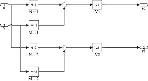
   Let the system observation matrix and input observation matrix in residual generator be represented as: (20) $\begin{array}{rl}{\mathbf{A}}_{L_d}& =\mathbf{A}-{\mathbf{L}}_d\mathbf{C},{\mathbf{B}}_{L_d}=\mathbf{B}-{\mathbf{L}}_d\mathbf{D}\end{array}$(20) (21) $\begin{array}{rl}{\mathbf{A}}_{L_f}& =\mathbf{A}-{\mathbf{L}}_f\mathbf{C},{\mathbf{B}}_{L_f}=\mathbf{B}-{\mathbf{L}}_f\mathbf{D}\end{array}$(21) Then, ${\mathbf{r}}_d$ and ${\mathbf{r}}_f$ are: (22) $\begin{array}{rl}{\mathbf{r}}_d\left(p\right)& ={\mathbf{V}}_1\left[\left(\mathbf{I}-\mathbf{C}{\left(p\mathbf{I}-{\mathbf{A}}_{L_d}\right)}^{-1}{\mathbf{L}}_d\right)\mathbf{y}\left(p\right)\right.\\ & \left.-\left(\mathbf{D}+\mathbf{C}{\left(p\mathbf{I}-{\mathbf{A}}_{L_d}\right)}^{-1}{\mathbf{B}}_{L_d}\right)\mathbf{u}\left(p\right)\right]\\ & ={\mathbf{V}}_1\left[{\hat{\mathbf{M}}}_1\left(p\right)\mathbf{y}\left(p\right)-{\hat{\mathbf{N}}}_1\left(p\right)\mathbf{u}\left(p\right)\right]\end{array}$(22) (23) $\begin{array}{rl}{\mathbf{r}}_f\left(p\right)& ={\mathbf{V}}_2\left[\left(\mathbf{I}-\mathbf{C}{\left(p\mathbf{I}-{\mathbf{A}}_{L_f}\right)}^{-1}{\mathbf{L}}_f\right)\mathbf{y}\left(p\right)\right.\\ & \left.-\left(\mathbf{D}+\mathbf{C}{\left(p\mathbf{I}-{\mathbf{A}}_{L_f}\right)}^{-1}{\mathbf{B}}_{L_f}\right)\mathbf{u}\left(p\right)\right]\\ & ={\mathbf{V}}_2\left[{\hat{\mathbf{M}}}_2\left(p\right)\mathbf{y}\left(p\right)-{\hat{\mathbf{N}}}_2\left(p\right)\mathbf{u}\left(p\right)\right]\end{array}$(23)

   Two residual generators connect together by cascading. Their common inputs are $\mathbf{u}$ and $\mathbf{y}$ and output are ${\mathbf{r}}_d$ and ${\mathbf{r}}_f$, respectively. The structure of residual generator is shown in Figure 4.

3.3. Fault-tolerant controller

The structure of double closed-loop is used to realize the integrated design of fault diagnosis and control. Inner loop consists of controlled devices, stable controller and robust controller for disturbance, which can ensure the stable work state of system and robustness for disturbance. Outer loop consists of inner loop and fault-tolerant controller which ensure the safety when fault occurs.

Figure 4. Structure of residual generator.

In order to analyse the performance of closed-loop system completely, we use the method of constructing integrated state-space. The inner loop is for stable controller and robust controller, and the disturbances on the system are fully considered. However, the outer loop is for active fault-tolerant controller, and the faults on the system are fully considered. As a result, some adjustments are required to build integrated state-space.

(1) The overall control law of the system is: (24) $\begin{array}{rl}u\left(p\right)& =u_1\left(p\right)+u_2\left(p\right)\\ & =F\hat{x}\left(p\right)+u_c\left(p\right)+V\left(w+u_w\left(p\right)\right)\end{array}$(24) where $u_1\left(p\right)=F\hat{x}\left(p\right)+u_c\left(p\right)$ is feedback control law, $u_c\left(k\right)=R_c\left(k\right)r_d\left(k\right)$ is robust control law, ${\mathbf{R}}_c\left(k\right)$ is transfer function of robust controller, ${\mathbf{u}}_2\left(p\right)=\mathbf{V}\left(\mathbf{w}+{\mathbf{u}}_w\left(p\right)\right)$ is feed-forward control law, and ${\mathbf{u}}_w\left(k\right)$ is fault-tolerant control law.

Dynamic controller is adopted as fault-tolerant controller. The integrated state space of outer loop is: (25) $\begin{array}{rl}\overline{\mathbf{x}}(p+1)& ={\overline{\mathbf{A}}}_F\overline{\mathbf{x}}\left(p\right)+\overline{\mathbf{B}}\overline{\mathbf{u}}\left(p\right)+\tilde{\mathbf{L}}\tilde{\mathbf{r}}\left(p\right)\end{array}$(25) (26) $\begin{array}{rl}\overline{\mathbf{u}}\left(p\right)& =\overline{\mathbf{K}}{\mathbf{x}}_{r_f}\left(p\right)\end{array}$(26) where $\overline{\mathbf{x}}\left(p\right)=\left[\hat{\mathbf{X}}\right(p\left){\mathbf{x}}_{r_f}\right(p){]}^T$ are states, $\tilde{\mathbf{r}}\left(p\right)=[\overline{\mathbf{r}}\left(p\right){\mathbf{r}}_f\left(p\right){]}^T$ are residuals, ${\overline{\mathbf{A}}}_F=\left[\begin{array}{cc}\mathbf{A}+\mathbf{B}\mathbf{F}& \mathbf{0}\\ \mathbf{0}& {\mathbf{G}}_{r_f}\end{array}\right]$ is system matrix, in which ${\mathbf{G}}_{r_f}$ meets ${\mathbf{A}}_{r_f}={\mathbf{G}}_{r_f}+{\mathbf{B}}_{r_f}{\mathbf{F}}_{r_f}$, $\overline{\mathbf{B}}=\left[\begin{array}{cc}\mathbf{B}& \mathbf{0}\\ \mathbf{0}& {\mathbf{B}}_{r_f}\end{array}\right]$ is input matrix, $\overline{\mathbf{L}}=\left[\begin{array}{cc}{\mathbf{L}}_1& \mathbf{0}\\ \mathbf{0}& {\mathbf{B}}_{r_f}\end{array}\right]$ is observation matrix, in which ${\mathbf{L}}_1=\left[\mathbf{L}{\mathbf{R}}_c\left(k\right)\right]$, $\overline{\mathbf{K}}=\left[\begin{array}{cc}{\mathbf{C}}_{r_d}^T& {\mathbf{F}}_{r_d}^T\end{array}\right]$ is the parameter set of fault-tolerant controller.

(2) Establish LQ tracker performance indicator. Feed-forward compensation of fault-tolerant controller is added to the given parameters of the system, which can realize track performance of the system: (27) $\begin{array}{rl}J& =\frac{1}{2}{\int }_0^{tf}\left({\mathbf{e}}^T\left(t\right){\mathbf{Q}}_f\mathbf{e}\left(t\right)+{\overline{\mathbf{u}}}^T\left(t\right){\mathbf{R}}_f\overline{\mathbf{u}}\left(t\right)\right)\mathrm{d}t\\ & =\frac{1}{2}{\int }_0^{tf}\left[{\left(\mathbf{w}-\mathbf{y}\left(t\right)\right)}^T{\mathbf{Q}}_f\left(\mathbf{w}-\mathbf{y}\left(t\right)\right)\right.\\ & \left.+{\overline{\mathbf{x}}}^T\left(t\right){\tilde{\mathbf{C}}}^T{\overline{\mathbf{K}}}^T{\mathbf{R}}_f\overline{\mathbf{K}}\tilde{\mathbf{C}}\overline{\mathbf{x}}\left(t\right)\right]\mathrm{d}t\end{array}$(27)

Minimum principle is used to solve the fault-tolerant control law: (28) $\begin{array}{rl}{\overline{\mathbf{u}}}^{\ast }\left(t\right)& =\overline{\mathbf{K}}\left(\mathbf{w}-\tilde{\mathbf{C}}{\overline{\mathbf{x}}}^{\ast }\left(t\right)-\mathbf{r}\left(t\right)\right)=\overline{\mathbf{K}}\left(\mathbf{w}-\mathbf{r}\left(t\right)\right)\\ & -\overline{\mathbf{K}}\tilde{\mathbf{C}}{\overline{\mathbf{x}}}^{\ast }\left(t\right)\end{array}$(28) where $\overline{\mathbf{K}}=-{\mathbf{R}}_f^{-1}{\overline{\mathbf{B}}}^T\mathbf{P}{\tilde{\mathbf{C}}}^T(\tilde{\mathbf{C}}{\tilde{\mathbf{C}}}^T{)}^{-1}$, $\mathbf{P}$ is the solution of Riccati differential equation, which can be calculated by the gradient method.

4. Simulation verification and analysis

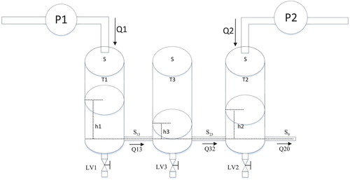
In this section, the developed framework will be applied to DST200 three-tank system, as shown in Figure 5. The fixed parameters of the three tank system are: tank bottom area $S=154\mathrm{c}{\mathrm{m}}^2$, maximum tank height $H_{max}$ = 62 cm, connecting pipe cross-sectional area $s=0.5\mathrm{c}{\mathrm{m}}^2$, flow coefficient $a_{z1}=0.45$, $a_{z2}=0.45$, $a_{z3}=0.6$, maximum pump flow $Q_{1max}=100\mathrm{c}{\mathrm{m}}^3/\mathrm{s}$, $Q_{2max}=100\mathrm{c}{\mathrm{m}}^3/\mathrm{s}$, gravity acceleration $g=981\mathrm{c}\mathrm{m}/{\mathrm{s}}^2$. The input variables are: pump flow $Q_1$ and $Q_2$, output variables are liquid level $h_1$, $h_2$, and $h_3$. State variable $\mathbf{x}={\left[\begin{array}{ccc}{h}_1& h_2& h_3\end{array}\right]}^T$, Control variable $\mathbf{u}={\left[\begin{array}{cc}{Q}_1& Q_2\end{array}\right]}^T$, System matrix $\mathbf{A}=\left[\begin{array}{ccc}-a_1& 0& a_1\\ 0& -\left(a_2+a_3\right)& a_3\\ a_1& a_3& -\left(a_1+a_3\right)\end{array}\right]$, where $a_1=a_{z1}{s}_{13}\sqrt{2g}/2\cdot S\cdot \sqrt{h_{10}-h_{30}}$, $a_2=a_{z2}{s}_0\sqrt{2g}/2\cdot S\cdot \sqrt{h_{20}}$, $a_3=a_{z3}{s}_{23}\sqrt{2g}/2\cdot S\cdot \sqrt{h_{30}-h_{20}}$, $b=1/S$, input matrix $\mathbf{B}=\left[\begin{array}{cc}b& 0\\ 0& b\\ 0& 0\end{array}\right]$, observation matrix $\mathbf{C}=\left[\begin{array}{ccc}1& 0& 0\\ 0& 1& 0\end{array}\right]$.

Figure 5. Structure diagram of three water tank DTS200.

4.1. Performance analysis of residual decoupling

Firstly, the disturbance and actuator faults were added to DTS200, which were used to simulate the disturbance and faults in actual production process. The disturbance was added in the front of sensor, and the range was $d\in \left(0,0.1\right)$. Actuator fault was the water pump failure in the three tank system, which reduced the flow rate. Supposed that at t=900s, the pump failure was $50\mathrm{\%}$, that is, fault factor $f_{A2}=0.5$, then ${\tilde{Q}}_1=\left(1-f_{A2}\right)Q_1$. When the disturbance and actuator fault were added, the system deviated from the normal working condition due to the disturbance of system. In the process of fault diagnosis, the residuals of the disturbance and the fault will be coupled together if the residuals were not decoupled. When the system did not carry out decoupling of residuals, residual outputs of two circumstances: (1) with disturbance and fault-free system and (2) with disturbance and fault are shown in Figure 6, respectively.

Figure 6. Comparison results of residual undecoupled. (a) Disturbance and no fault and (b) disturbance and fault.

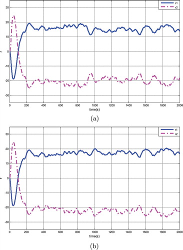
As can be seen fromFigure 6, due to the coupling of disturbance and fault, when the fault occurs, the residual is still in irregular fluctuations. It means that the fault cannot be accurately diagnosed. As a result, the residuals need to be decoupled. According to the aforementioned method, analysis of residual decoupling according to the state space model, and construction of special residual generator reflect the disturbance residual ${\mathbf{r}}_{\mathbf{d}}$ on the system and the fault residual ${\mathbf{r}}_{\mathbf{f}}$ on the system, respectively.

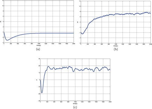
Figure 7 shows the residual of the system in three circumstances, i.e. no disturbance and fault, fault and on disturbance and disturbance and fault.

Figure 7. Simulation results of residual $r_d$. (a) No disturbance and fault, (b) fault and on disturbance and (c) disturbance and fault.

4.2. Simulation and analysis of robust control and fault-tolerant control

(1) Simulation and analysis of robust control

Robust control is mainly designed to ensure that the system is robust to disturbance. Residual ${\mathbf{r}}_{\mathbf{d}}$ is input and robust control law ${\mathbf{u}}_{\mathbf{c}}$ is output. Let weight $Q_d=\left(1,1,1,15,15\right)$, $R_d=\left(0.5,0.5,0.5\right)$, parameter matrix ${\overline{K}}_{rd}=\left[\begin{array}{cc}0.7351& 0\\ -0.6616& -0.7351\\ -2.1125& -2.3569\end{array}\right]$ can be calculated. Thus, parameters of the dynamic controller are as follow: ${\mathrm{A}}_{rd}=\left[\begin{array}{cc}0& 1\\ -2.1125& -2.3569\end{array}\right]$, ${\mathrm{B}}_{rd}=\left[\begin{array}{c}0\\ 1\end{array}\right]$, ${\mathrm{C}}_{rd}=\left[\begin{array}{cc}0.7351& 0\\ -0.6616& -0.7351\end{array}\right]$.

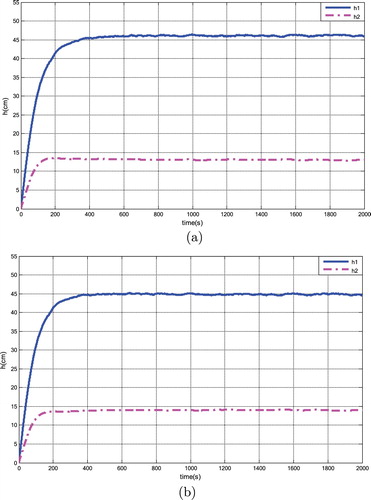
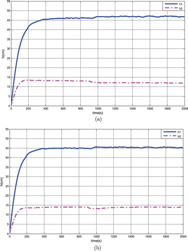
In case of disturbances and fault-free, system outputs before and after robust control are shown in Figure 8(a,b), respectively. It can be seen that after robust control, the output of the system can return normal working status and overcome the effects of disturbance, that is, the system is robust to disturbance and control objective can be obtained.

Figure 8. System outputs before and after robust control. (a) Before robust control and (b) after robust control.

(2) Simulation and analysis of fault-tolerant control

Fault-tolerant control is mainly designed to improve the fault tolerance ability. Residual $r_f$ is input and fault-tolerant control law ${\mathbf{u}}_{\mathbf{w}}$ is output. The given parameters can be automatically adjusted when faults occur. Let weight $Q_f=\left(10,10\right),R_f=\left(0.5,0.5,0.5\right)$, parameter matrix ${\overline{K}}_{rf}=\left[\begin{array}{cc}0.8154& 0\\ -0.7746& -0.8154\\ -1.5595& -1.7271\end{array}\right]$ can be calculated. Thus, parameters of the dynamic controller are as follow: ${\mathrm{A}}_{rf}=\left[\begin{array}{cc}0& 1\\ -1.5595& -1.7271\end{array}\right]$, ${\mathrm{B}}_{rf}=\left[\begin{array}{c}0\\ 1\end{array}\right]$, ${\mathrm{C}}_{rf}=\left[\begin{array}{cc}0.8154& 0\\ -0.7746& -0.8154\end{array}\right]$. In case of fault but without disturbance, system outputs before and after fault-tolerant control are shown in Figure 9(a,b), respectively.

Figure 9. System outputs before and after fault-tolerant control. (a) Before fault-tolerant control and (b) after fault-tolerant control.

It can seen that after fault-tolerant control, the output of the system can return normal working status and achieve good fault-tolerant performance by means of adjusting the given parameters.

4.3. Simulation and analysis of integrated design

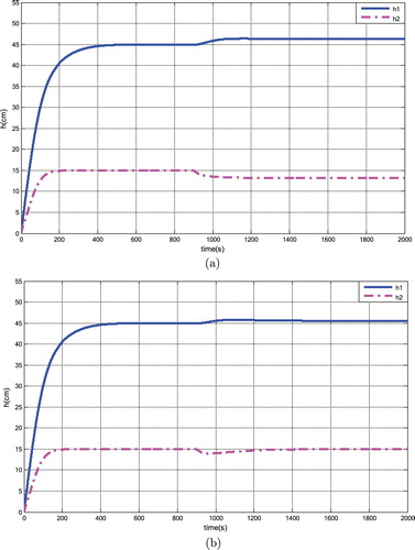
System outputs before and after robust and fault-tolerant controls are shown in Figure 10(a ,b), respectively. It can seen that robust and fault-tolerant controls can ensure the output of the system remain normal working status by means of robust control for disturbance and fault-tolerant control for fault.

Figure 10. System outputs before and after robust and fault-tolerant controls. (a) Before robust and fault-tolerant controls and (b) after robust and fault-tolerant controls.

Based on the above results, it can be concluded that the performance and effect of integrated design can be summed up as follows:

1. In terms of performance, the system is designed based on state space model analysis. First of all, residual ${\mathbf{r}}_d$ and residual ${\mathbf{r}}_f$ are generated by residual decoupling, which reflect the influence of disturbance and fault on the system, respectively. Then, the optimal robust controller is designed by means of feedback control, which ensure the system is robust to disturbance. At the same time, optimal fault-tolerant controller is designed by adjusting the given parameters which introduces feed-forward control into the system to ensure the system is fault tolerance.

2. In terms of fault diagnosis, the accuracy of diagnosis is increased due to the complete residual decoupling for disturbance. The real-time performance of diagnosis is improved by proper design of evaluation function and threshold.

3. In terms of integrated design, the function of fault diagnosis is tactfully integrated into the control system by built-in residual generator and residual evaluation module. The overall operation of process control and fault diagnosis can be carried out. The operation security of the system is strengthened due to fault-tolerant control.

5. Conclusion

In this paper, an integrated framework for fault diagnosis and control has been designed based on residual decoupling technology. Based on this novel scheme, the robustness of control system and the sensitivity of fault diagnosis system have been fully considered. Firstly, the decoupling technology was used for separation of fault and disturbance. Then, robust controller and fault-tolerant controller were designed for rejecting the system disturbance and guaranteeing the system performance, respectively. Finally, the proposed methods were applied to three-tank system to demonstrate the performance and effectiveness. Future work will be dedicated to expanding the proposed integrated design scheme into nonlinear system.

Disclosure statement

No potential conflict of interest was reported by the authors.

ORCID

Jie Dong  http://orcid.org/0000-0001-8314-3047

Additional information

Funding

This work was supported by the Natural Science Foundation of China (NSFC) [grant numbers 61873024, 61773053, 61673032] and by Fundamental Research Funds for the China Central Universities of USTB [grant number FRF-BD-18-002A, FRF-GF-17-A4], People's Republic of China. Also thanks for the National Key R&D Program of China [grant number 2017YFB0306403] for funding.

References

- Ding, S. X. (2009). Integrated design of feedback controllers and fault detectors. Annual Reviews in Control, 33(2), 124–145. doi: 10.1016/j.arcontrol.2009.08.003
- Ding, S. X. (2013). Model-based fault diagnosis techniques-design schemes, algorithms and tools. 2nd ed. London: Springer-Verlag.
- Ding, S. X. (2014). Data-driven design of fault diagnosis and fault-tolerant control systems. London: Springer-Verlag.
- Diversi, R., & Simani, S. (2013). Residual design for dynamic processes using decoupling technique. In 42nd IEEE International Conference on Decision and Control (1, pp. 451–456), Maui, HI, USA.
- Ge, Z. Q., Song, Z. H., & Gao, F. R. (2013). Review of recent research on data-based process monitoring. Industrial and Engineering Chemistry Research, 52, 3543–3562. doi: 10.1021/ie302069q
- Gertler, J. J., & Kunwer, M. M. (1995). Optimal residual decoupling for robust fault diagnosis. International Journal of Control, 61(2), 395–421. doi: 10.1080/00207179508921908
- Isermann, R. (2006). Fault diagnosis systems: An introduction from fault detection to fault tolerance. London: Springer-Verlag.
- Lan, J., & Patton, R. J. (2018). A decoupling approach to integrated fault-tolerant control for linear systems with unmatched non-differentiable faults. Automatica, 89, 290–299. doi: 10.1016/j.automatica.2017.12.011
- Li, L. L., Luo, H., Ding, S. X., Yang, Y., & Peng, K. X. (2019). Performance-based fault detection and fault-tolerant control for automatic control systems. Automatica, 99, 308–316. doi: 10.1016/j.automatica.2018.10.047
- Li, S., Wang, Z. D., Wang, W. B., & Alsaadi, F. E. (2017). Output-feedback control for nonlinear stochastic systems with successive packet dropouts and uniform quantization effects. IEEE Transactions on Systems, Man, and Cybernetics: Systems, 47(7), 1181–1191.
- Ma, L., Dong, J., Peng, K. X., & Zhang, C. F. (2019). Hierarchical monitoring and root cause diagnosis framework for key performance indicator-related multiple faults in process industries. IEEE Transactions on Industrial Informatics, 15(4), 2091–2100. doi: 10.1109/TII.2018.2855189
- Paoli, A., Matteo, S., & Stéphane, L. (2011). Active fault tolerant control of discrete event systems using online diagnostics. Automatica, 47(4), 639–649. doi: 10.1016/j.automatica.2011.01.007
- Shen, B., Ding, S. X., & Wang, Z. D. (2013). Finite-horizon H∞ fault estimation for linear discrete time-varying systems with delayed measurements. Automatica, 49(1), 293–296. doi: 10.1016/j.automatica.2012.09.003
- Tidriri, K., Chatti, N., Verron, S., & Tiplica, T. (2016). Bridging data-driven and model-based approaches for process fault diagnosis and health monitoring: A review of researches and future challenges. Annual Reviews in Control, 42, 4263–4281. doi: 10.1016/j.arcontrol.2016.09.008
- Xiang, Y., Li, P., & Zhang, Y. M. (2018). The design of fixed-time observer and finite-time fault-tolerant control for hypersonic gliding vehicles. IEEE Transactions on Industrial Electronics, 65(5), 4135–4144. doi: 10.1109/TIE.2017.2772192
- Yin, S., Ding, S. X., Xie, X. C., & Luo, H. (2014). A review on basic data-driven approaches for industrial process monitoring. IEEE Transactions on Industrial Electronics, 61(11), 6418–6428. doi: 10.1109/TIE.2014.2301773
- Yin, S., Wang, G., & Yang, X. (2014). Robust PLS approach for KPI-related prediction and diagnosis against outliers and missing data. International Journal of Systems Science, 45(7), 1375–1382. doi: 10.1080/00207721.2014.886136
- Zhang, P., & Ding, S. X. (2007). Disturbance decoupling in fault detection of linear periodic systems. Automatica, 43(8), 1410–1417. doi: 10.1016/j.automatica.2007.01.005
- Zhang, Y. M., & Jiang, J (2001). Integrated active fault-tolerant control using IMM approach. IEEE Transactions on Aerospace and Electronic Systems, 37(4), 1221–1235. doi: 10.1109/7.976961
- Zhang, X. D., Marios, M. P., & Thomas, P. (2002). A robust detection and isolation scheme for abrupt and incipient faults in nonlinear systems. IEEE transactions on automatic control, 47(4), 576–593. doi: 10.1109/9.995036
- Zhang, Y., Yang, Y., Ding, S. X., & Li, L. L. (2016). Optimal design of residual-driven dynamic compensator using iterative algorithms with guaranteed convergence. IEEE Transactions on Systems Man and Cybernetics: Systems, 46(4), 548–558. doi: 10.1109/TSMC.2015.2450203
- Zhou, K. M., & Zhang, R. L. (2001). A new controller architecture for high performance, robust, and fault-tolerant control. IEEE Transactions on Automatic Control, 46(10), 1613–1618. doi: 10.1109/9.956059