Optimal electric business centre location by centre–decentre quantum particle swarm optimization

Abstract

This paper proposes an electric business centre location model solved by centre–decentre quantum particle swarm optimization (CDQPSO). Firstly, a location model is built taking real factors into accounts such as the cost of business centres and consumers, the competitive relationship between newly built and existing ones, and their service qualities. Secondly, in order to solve the location model, a CDQPSO algorithm is proposed by the combination of centralized–decentralized learning and the motion mode of the quantum bound state particle. Benchmark experiments on the proposed CDQPSO and existing PSO algorithms indicate that the proposed algorithm has better performance. Finally, CDQPSO is applied to solve the locations of business centres. Compared with the existing methods, the new-built business centre of our proposed method can provide consumers with higher transportation convenience and service quality. Moreover, the power company can reduce the construction cost of business centres and improve social benefits.

KEYWORDS:

• Business centre
• location optimization
• centre–decentre learning
• Particle Swarm Optimization

1. Introduction

Business centre, such as electric business centre, bank branch, and convenience store, is one of the main places to provide service and communicate with consumers. It plays a vital role in enhancing the reputation of a company. Therefore, it is crucial to treat the location of a business centre as a long-term investment.

The uneven distribution of the population in different regions has led to significant differences in service pressure of business centres. Along with the prevalent of urbanization, the problems caused by the irrational distribution of business centre have become increasingly prominent. On the one hand, some business centres need to be cancelled or merged due to insufficient business demand to reduce the company’s costs. On the other hand, new industrial or science parks and residential areas need to be covered by new business centres to improve service quality. However, most existing models about business centre concentrate on efficiency (Cvetkoska & Savic, 2017; Quaranta, Raffoni, & Visani, 2018), service quality (Ferreira, Jalali, Ferreira, Stankeviciene, & Marques, 2015), and demand forecast (Cabello & Lobillo, 2016; Da, Kun, & Han, 2018). Few models pay attention to the location optimization of the business centre, which can help companies reduce costs and improve efficiency. Colledani and Battaia (2016) proposed a decision support system helps to make decisions about the depth of disassembly and the organization of the disassembly system. Moreover, it improves the robustness of the disassembly process. In this paper, we propose a reasonable location model to help decision-making for future business centre location, which will realize the optimal economic and social benefits with regard to satisfying the demands of consumers.

The location problem has been proposed and studied for a long time. Hakimi conducted more systematic and theoretical research on the location problem in 1964 (Hakimi, 1964). Since then, more and more scholars are attracted by this problem as new scenarios, and new methods are emerging. Literature (2010) provides a review on the recent development in multi-criteria location problems in three categories including bi-objective (Abdelaziz, El-Sharkawy, & Attia, 2011; Bhaskaran & Turnquist, 1990; Blanquero & Carrizosa, 2002; Kozanidis, 2009; Villegas, Palacios, & Medaglia, 2006), multi-objective (Araz, Selim, & Ozkarahan, 2007; Diabat, Abdallah, Al-Refaie, Svetinovic, & Govindan, 2013; Hsieh, Yu, & Wang, 2008; Kumar & Gao, 2009, Sen, Sen, & Diwekar, 2016) and multi-attribute (Aras, Erdogmus, & Koc, 2004; Chan & Chung, 2004; Fernandez & Ruiz, 2009; Tuzkaya, Onut, Tuzkaya, & Gulsun, 2008) problems. In bi-objective problems, Kozanidis (2009) have introduced the convex Linear Multiple Choice Knapsack Problem that incorporates a second objective to allocate the available resource among a group of disjoint sets of activities, equitably. Villegas et al. (2006) modelled a supply network as a bi-objective location problem, with minimum and maximum objectives for construction costs and service coverage. Abdelaziz et al. (2011) present an approach to find the optimal location of the thyristor-controlled series compensators in a power system to improve the load ability of its lines and minimize its total loss. In multi-objective problems, Kumar and Gao (2009) proposed a new price-area-based zonal approach for the optimal location of distributed generation in a pool. Araz et al. (2007) proposed a coverage-based fuzzy multi-objective model aiming at solving the location of emergency service centre with Euclidean distances. Optimal sensor location problem in Integrated Gasification Combined Cycle (IGCC) power plants was solved by Pallabi et al. (2016). In multi-attribute problems, Tuzkaya et al. (2008) used the analytic network process (ANP) technique to analyze location problem based on four primary factors (benefits, costs, opportunities and risks). Aras et al. (2004) considered the location of wind observing station under multiple criteria. Fernandez and Ruiz (2009) solved the location problem of the industrial park through a three-level hierarchical decision process.

The location problem is a nonlinear optimization problem, which is difficult to obtain an analytical solution. Therefore, the heuristic method is suitable for solving it. In many recent papers, heuristic techniques have been used to solve the location problem. Lin and Kwok (2006) applied Tabu Search and Simulated Annealing to solve location problem, and compared their performance through a statistical programme. Stummer, Doerner, Focke, and Heidenberger (2004) extended the original Tabu Search algorithm to allow decision makers to interactively explore the solution space to determine the ‘‘best’ configuration. Gomez, Jurado, Diaz, and Ruiz-Reyes (2010) proposed a particle swarm optimization-based method for the optimal location of the photovoltaic grid-connected system.

Particle swarm optimization (PSO) algorithm is a heuristic algorithm which was proposed based on the social behaviours of fish and birds in 1995 by Kenedy and Eberhart (1995). It is a swarm stochastic optimization technique, and a particle swarm is composed of multiple particles. Each particle represents a feasible solution in the solution space. In each iteration, the position of a particle is updated according to the individual optimum (individual experience) and global optimum (social experience) of particle swarm. When the iteration stops, all particles will gather in a specific area in the solution space and find the optimal solution (Kenedy & Eberhart, 1995). Sun, Xu, and Feng (2005) used the knowledge in quantum mechanics and proposed quantum particle swarm optimization (QPSO) algorithm to overcome the shortcomings of PSO which cannot cover the whole available area. Zhang, Liu, Meng, Yang, and Vasilakos (2017) proposed centre–decentre particle swarm optimization (CDPSO) algorithm by combining the PSO algorithm with centralized learning and decentralized learning to increase the abundance of particle swarm.

PSO algorithm has the advantages of high efficiency and easy implementation. However, sometimes it is easy to fall into local optimum (Bergh, 2006; Bergh & Engelbrecht, 2002). In this paper, considering many factors, an electric business centre location model was established. In order to get a better solution, a new heuristic algorithm CDQPSO was proposed by combining QPSO algorithm and CDPSO algorithm, which is applied to solve the electric business centre location model.

The main contribution of the paper can be summarized as follows:

1. An electric business centre location model which considers many actual factors is proposed.

2. An improved particle swarm optimization algorithm is proposed to solve the location model.

2. Electric business centre location modelling

In this section, the location model of the business centre is established based on the actual scene. Lots of factors should be considered when locating a business centre. The factors are divided into two categories. One kind is positive factors that are expected to have a maximum value during the location process, as shown in formula (1). The other kind is negative factors that are expected to have a minimum value, as shown in formula (2),$(x,y)$ is the coordinate of the business centre. (1) $\begin{array}{rl}& P(x,y)\end{array}$(1) (2) $\begin{array}{rl}& N(x,y)\end{array}$(2)

In order to effectively integrate two kinds of factors, the objective function of the model in this paper is as follows: $\begin{array}{rl}F& =\frac{{\sum }_{i=1}^m{\omega }_N^i\frac{\left(1+N^i(x,y)\right)}{{\sigma }_N^i}}{{\sum }_{j=1}^n{\omega }_P^j(1+P^j(x,y\left)\right){\sigma }_P^j}\end{array}$ (3) $\begin{array}{rl}& s.t.x_{min}<x<x_{max}\end{array}$(3) $\begin{array}{rl}& y_{min}<y<y_{max}\end{array}$where ${\sigma }_N^i$ represents the standard deviation of $N^i(x,y)$ for the i-th negative factor. It embodies the normalization process of factors, which eliminates the magnitude differences between different factors. ${\omega }_N^i$ represents the weight of the i-th factor. The weights vary in different realistic scenarios according to consumer’s preference. $n,m$ represents the number of positive and negative factor. The objective of the location problem is to find a position $(x,y)$ within a limited range to minimize the objective function $F$. This paper focuses on the factors of the competitive relationship between business centres, transportation convenience, and construction cost.

2.1. Competitive relationship between business centres

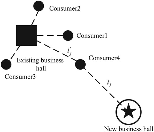
Different business centres have different abilities to attract consumers. The attraction will decrease with distance increases. The number of consumers directly determines their business pressure. Each business centre has a normal pressure range. Once the pressure exceeds the standard value, its service quality will be affected. Through optimization, the model will choose a location to make the pressure of each business centre more balanced. In this paper, business centre service quality is calculated as follows (Figure 1): (4) $Q_i(x,y)=\frac{|H_i(x,y)-{\overline{H}}_{is}|}{H_{is}}$(4) where $Q_i(x,y)$ represents service quality of business centre $i$,$H_i(x,y)$ represents the total number of consumers around business centre $i$,${\overline{H}}_{is}$ represents the standard number of consumers to provide service for business centre $i$. $H_i(x,y)$ is determined by: (5) $\begin{array}{rl}{H}_i(x,y)& =\sum _{j=1}^l(w\times h_j)\end{array}$(5) (6) $\begin{array}{rl}w& =\left\{\begin{array}{l}1,\text{if}0.5-\frac{l_j}{l_j^{\mathrm{\prime }}}\times \text{rand}\left(\right)>0\\ 0,else\end{array}\right.\end{array}$(6) where $l$ represents the number of consumer groups belong to business centre $i$ at previous iteration, $h_j$ represents the number of consumers in $j$ group,$w$ is a criterion used to judge whether the consumers in $j$ group belong to business centre $i$. If $w$ equals 1, then consumers in $j$ group belong to business centre i. $l_j^{\mathrm{\prime }}$ represents the distance between consumer group $j$ and the business centre in the previous iteration, $l_j$ represents the distance between consumer group $j$ and newly built business centre, $\text{rand}\left(\right)$ is a random function between 0 and 1 that represents the randomness of consumer selection. According to Formula (6), the consumer choice of the business centre is affected by the distance between the centre and its position. If the consumer has the same distance to the two business centres, then he will randomly choose one of them.

Figure 1. The influences of new business centre on existing business centre.

A good location of the new business centre will make the total centres’ pressure more balanced. This paper uses formula (7) to calculate the average score of service quality of all business centres after the establishment of a new business centre. (7) $Q(x,y)=\frac{1}{M}\ast \sum _i^u{Q}_i(x,y)$(7) where $M$ represents the total number of business centres, and the smaller $Q(x,y)$, the better layout of the new business centre.

2.2. Transportation convenience

Transportation convenience is usually related to the number of bus stops and subway stations around the business centre. The more they are, the more convenient business centre is. Consumers prefer to choose a more convenient business centre. In this paper, as shown in formula (8) and formula (9), the convenience is evaluated by the number of bus stops within $D_1$ kilometres around it, and the number of subway stations within $D_2$ kilometres around it. (8) $\begin{array}{rl}B(x,y)& =\sum _{i=1}^{N_b}{b}_i\end{array}$(8) (9) $\begin{array}{rl}S(x,y)& =\sum _{j=1}^{N_s}{s}_j\end{array}$(9) where $B(x,y)$ represents the number of bus stops, and$S(x,y)$ represents the number of subway stations. If the distance between bus stop $i$ and business centre is less than $D_1$ then the value of $b_i$ is 1. Otherwise, the value is 0. $N_b$ represents all bus stops in the target area, and $N_s$ represents all subway stations.

Similarly, $S(x,y)$ is obtained by count all the subway stations within $D_2$ kilometres.

2.3. Construction cost

The construction cost of the business centre is mainly determined by the rent of the office since the device cost, and labour cost is similar among different centres. In this paper, the candidate area will be partitioned into many small blocks, and each block is assigned to an economic cost index $E(x,y)$. For simplicity, the economic cost index is divided into ten levels according to the actual situation.

3. Centre–decentre quantum particle swarm optimization algorithm

3.1. Proposed algorithm

Particle swarm optimization (PSO) is an optimization algorithm based on swarm intelligence theory and originates from the simulation of the birds feeding process. Through the competition between individuals, dominant individuals are produced. And dominant individuals guide the rest individuals to search and evolve. Particle swarm optimization has the advantages of high efficiency and easy implementation. However, sometimes it is easy to fall into a local optimum. In the PSO algorithm, the particle’s motion mode is determined by moving velocity. The moving velocity of particles is limited. The search space in an iteration is a limited area which cannot cover the whole available area. This conclusion has been proved by F. van den Bergh (Bergh, 2006; Bergh & Engelbrecht, 2002). In order to overcome the shortcomings of PSO, Sun et al. (2005) used the knowledge in the quantum mechanics and proposes quantum particle swarm optimization (QPSO) algorithm. The particles in quantum bound state appear at any point in space with a certain probability density. It requires that when the distance between the particle and centre is going to infinity, the probability density approaches zero. Like other algorithms based on swarm intelligence optimization, when the QPSO swarm converges into a smaller range, the diversity will decrease, and when solving complex multimodal problems, QPSO algorithm may fall into a local optimum.

Zhang et al. (2017) proposed a centre–decentre particle swarm optimization (CDPSO) algorithm based on centralized–decentralized learning to solve the premature convergence problem. Centralized learning is a depth search method that simulates the imitation of ordinary individuals from elite individuals in real society. Decentralized learning is a breadth search method based on the characteristics of individual distributed learning in society. Two methods complement each other in the search process, which better trades off the capabilities of global search and local search. CDPSO algorithm reduces the possibility of premature convergence. The movement state of CDPSO particles is determined by particle position and velocity. Generally, larger particle velocity leads to a larger particle search span and stronger global search ability. However, it is easy to miss the optimal solution when particle velocity is too large. Smaller particle velocity leads to stronger local search ability and a higher probability of falling into a local optimum. The control of velocity will have an obvious impact on the optimization of CDPSO algorithm in different scenarios, which will increase the difficulty of parameter tuning.

This paper proposes a centre–decentre quantum particle swarm optimization (CDQPSO) algorithm based on the centralized–decentralized learning of CDPSO algorithm and the motion mode of the quantum bound state particle of QPSO algorithm. This algorithm can increase diversity and reduce the probability of falling into a local optimum. At the same time, it avoids the influence of particle velocity on the performance of the algorithm.

Particle$i$ in bound state is attracted by $p_i=(p_{i,1},p_{i,2},\dots ,p_{i,n})$ during convergence, and the formulas are as follows. (10) $\begin{array}{rl}{p}_{i,j}\left(t\right)& =\frac{c_1{r}_{1,i,j}\left(t\right)P_{i,j}\left(t\right)+c_2{r}_{2,i,j}\left(t\right)G_j\left(t\right)}{c_1{r}_{1,i,j}\left(t\right)+c_2{r}_{2,i,j}\left(t\right)}i\le j\le N\end{array}$(10) (11) $\begin{array}{rl}{p}_{i,j}\left(t\right)& ={\varphi }_{i,j}\left(t\right)P_{i,j}\left(t\right)+\left[1-{\varphi }_{i,j}\left(t\right)\right]G_j\left(t\right)\end{array}$(11) (12) $\begin{array}{rl}{\varphi }_{i,j}\left(t\right)& =\frac{c_1{r}_{1,i,j}\left(t\right)}{\left[c_1{r}_{1,i,j}\left(t\right)+c_2{r}_{2,i,j}\left(t\right)\right]}\end{array}$(12) where ${\varphi }_{i,j}\left(t\right)$ is a uniformly distributed random number in interval (0,1), $i$ represents the $i\text{ - }$th particle, $j$ represents the dimension of particle, $P\left(t\right)$ is the individual optimal particle, $G\left(t\right)$ is globally optimal particle. The motion equation of particle’s one-dimensional $\delta$ potential well is as follow. (13) $X=p\pm \frac{L}{2}\ln \left(1/\mu \right)\mu \sim U(0,1)$(13) where $L$ represents the characteristic length of $\delta$ potential well, it is constantly decreasing in the process of evolution. The Particle $i$ stays near $p$ and eventually falls into $p$. Formula (13) describes the basic evolutionary process of QPSO. In quantum space, particles have no velocity vector and are only determined by the position formula shown below. (14) $\begin{array}{rl}{X}_{i,j}\left(t+1\right)& =p_{i,j}\left(t\right)\pm \alpha |C_j\left(t\right)\\ & -X_{i,j}\left(t\right)|\ast \ln \left[1/{\mu }_{i,j}\right(t\left)\right]{\mu }_{i,j}\left(t\right)\sim U(0,1)\end{array}$(14) where $i$ represents the $i\text{ - }$th particle. $j$ represents the dimension of particle, $\alpha$ is a contraction expansion factor that linearly decreases from 1.0 to 0.5 with iteration increasing $C_j\left(t\right)$ represents the average optimal position of particles in current iteration. The formula is as follow. (15) $C_j\left(t\right)=\frac{1}{M}\sum _{i=1}^M{P}_{i,j}\left(t\right)$(15)

Centralized–decentralized learning is added in the particle iteration process. The formulas are as follows. (16) $\left\{\begin{array}{l}{X}_{i,j}\left(t+1\right)=p_{i,j}\left(t\right)\pm \alpha |{\text{Center}}_i^j\left(t\right)-X_{i,j}\left(t\right)|\ast \ln \left[\frac{1}{{\mu }_{i,j}\left(t\right)}\right]\\ {\text{Center}}_i^j\left(t\right)=\frac{1}{L}\sum _{i=1}^L{P}_{i,j}\left(t\right)\\ {\mu }_{i,j}\left(t\right)\sim U\left(0,1\right)\end{array}\right.$(16) where ${\text{Center}}_i^j\left(t\right)$ represents the arithmetic mean of individual optimal positions of the top N particles with the best fitness. It embodies the idea of evolving swarm led by elite particles. (17) $\left\{\begin{array}{l}{X}_{i,j}\left(t+1\right)=p_{i,j}\left(t\right)\pm \alpha |P_{{\gamma }_i\left(j\right),j}-X_{i,j}\left(t\right)|\ast \ln \left[\frac{1}{{\mu }_{i,j}\left(t\right)}\right]\\ {\gamma }_i\left(j\right)=\text{rand}\left(\right)\mathrm{\%}N{\gamma }_i\left(j\right)\in [1,N]\\ {\mu }_{i,j}\left(t\right)\sim U\left(0,1\right)\end{array}\right.$(17) where ${\gamma }_i\left(j\right)$ represents the number of particles that particle $i$ learned in the $j\text{ - }$th dimension, $P_{{\gamma }_i\left(j\right)}$ represents the individual optimal position of selected particle; $N$represents the total number of particles. Firstly, two particles were randomly taken from the swarm and the particles with better fitness were selected as the learning objective of the current particle $i$. Decentralized learning can increase the diversity of swarm and reduce the probability of falling into a local optimum. 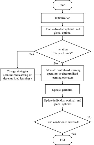CDQPSO algorithm alternately applies two particle updating strategies with period $\tau$ in the iterative process. Finally, CDQPSO algorithm is performed according to the following steps, and the flowchart is given in Figure 2.

• Step1: Set $t=0$ and initialize the current position of each particle $X_i\left(t\right)$.

• Step2: Calculate the fitness of particles.

• Step3: Find individual optimal $P\left(t\right)$ and global optimal $G\left(t\right)$.

• Step4: Determine whether the number of iterations of the current iteration strategy reaches $\tau$ times.

• Step5: Calculate centralized learning operators or decentralized learning operators.

• Step6: Update current particles position.

• Step7: Update individual optimal $P\left(t\right)$ and global optimal $G\left(t\right)$.

• Step8: If end condition (fitness value is good enough or reaching the maximum number of iterations $t_{max}$) is not satisfied, then$t=t+1$ and return Step3.

Figure 2. Flowchart of CDQPSO.

3.2. Algorithm evaluation

3.2.1. Comparison of optimization accuracy

In order to evaluate the global search ability of the proposed algorithm, four benchmark functions were selected to test the performance of the proposed algorithm. $F_2$ and $F_3$ are unimodal functions, and $F_1$ and $F_4$ are multimodal functions. The algorithm takes objective function value $f\left(x\right)$ as the fitness value. Table 1 lists the name, expression, searching scope of each dimension, and the global optimal value of each function.

Table 1. The formulae of the test benchmark functions.

Name	Objective	Global minimum	Modality
Rastrigin	$F_1=\sum _{i=1}^D(x_i^2-10\cos (2\pi x_i)+10)$	0	Multimodal
Rosenbrock	$F_2=\sum _{i=1}^D\left(100\right(x_{i+1}-x_i^2)+(1-x_i{)}^2)$	0	Unimodal
Sphere	$F_3=\sum _{i=1}^D\left|x^2\right|$	0	Unimodal
Alpine	$F_4=\sum _{i=1}^D|x_i\sin (x_i)+0.1x_i|$	0	Multimodal

In order to verify the performance of the algorithm on test function with different dimensions, four kinds of dimensions were randomly selected: 2-dimensional, 5-dimensional, 10-dimensional and 20-dimensional. The parameters of each algorithm are presented in Table 2. The parameter is the best one selected from the results of experiments. In order to reduce the error caused by chance, the experiment is repeated 15 times for each test function. The size of each swarm was uniformly set to 40, and the number of iterations can be calculated by the formula (18). $N_{\text{iter}}$ represents the number of iterations. $D$ represents the dimension. $N_{\text{particle}}$ represents the number of particles. On the one hand, with the increase of dimensions, the difficulty of optimization increases, so the number of iterations should be increased. On the other hand, the number of particles will increase computational complexity, but it will be easier to obtain global optimization solution. Therefore, as the number of particles increases, the number of iteration will decrease. The average, best, worst, and variance of the global optimal particle fitness are illustrated in Tables 3 and 4. The results of average optimal fitness have been highlighted in the tables. (18) $N_{\text{iter}}=\frac{D\ast 10000}{N_{\text{particle}}}$(18)

Table 2. Parameters settings of the involved algorithms.

Algorithms	Parameter settings
PSO	$\omega =0.8,c_1=2.0,c_2=2.0$
QPSO	$\alpha =1.0\sim 0.5,\mu \in [0,1]$
CDPSO	${\omega }_1=0.721,c_1=2.0,{\omega }_2=0.60,c_2=2.0,\tau =5$
CDQPSO	$\alpha =1.0\sim 0.5,\mu \in [0,1]$, ${\omega }_1=0.721,c_1=2.0,{\omega }_2=0.60,c_2=2.0,\tau =5$

Table 3. Comparison between several algorithms on 4 benchmark functions (1).

Algorithm		PSO	QPSO	PSO	QPSO	PSO	QPSO	PSO	QPSO
Dimension	Function	Best		Worst		Mean		Variance
2-D	F1	1.07E−8	0	3.73E−3	7.26E−6	2.57E−4	1.05E−6	9.28E−4	2.22E−6
	F2	1.26E−4	3.54E−10	6.35E−2	2.41E−6	1.44E−2	2.02E−7	1.61E−2	5.95E−7
	F3	1.67E−8	8.23E−49	6.01E−5	6.84E−39	9.12E−6	4.57E−40	1.51E−5	1.70E−39
	F4	4.08E−7	2.61E−9	1.56E−3	1.16E−4	2.26E−4	2.18	3.92E−4	3.74E−5
5-D	F1	1.88E−4	0	7.9E−2	1.79E−3	6.95E−3	2.77E−4	1.94E−2	5.69E−4
	F2	3.21E−2	2.20E−2	2.07	0.29	1.28	0.12	0.60	8.57E−2
	F3	3.08E−6	1.15E−181	8.12E−4	6.48E−167	2.46E−4	4.41E−168	2.35E−4	0
	F4	5.16E−5	5.18E−59	2.74E−2	5.61E−5	2.97E−3	6.61E−6	6.64E−3	1.58E−5
10-D	F1	6.66	0	22.45	3.07	15.2	1.21	4.87	0.99
	F2	6.65	0.63	97.32	2.94	31.73	1.70	26.77	0.59
	F3	0.84	8.58E−160	22.31	3.30E−134	5.77	2.28E−135	5.60	8.22E−135
	F4	0.14	7.35E−33	1.67	6.36E−21	0.67	1.44E−21	0.45	2.19E−21
20-D	F1	58.77	2.98	105.81	9.94	83.21	5.98	15.75	1.99
	F2	861.86	1.35	5619.61	68.92	2691.20	13.79	1355.35	14.92
	F3	179.79	8.20E−106	1513.10	6.01E−94	722.04	4.01E−95	361.83	1.49E−94
	F4	3.65	2.05E−18	9.27	3.05E−11	6.23	2.03E−12	1.39	7.65E−12

Table 4. Comparison between several algorithms on 4 benchmark functions (2).

Algorithm		CDPSO	CDQPSO	CDPSO	CDQPSO	CDPSO	CDQPSO	CDPSO	CDQPSO
Dimension	Function	Best		Worst		Mean		Variance
2-D	F1	0	0	0	0	0	0	0	0
	F2	2.94E−10	1.51E−10	1.67E−6	1.89E−8	2.14E−7	5.25E−9	4.15E−7	6.08E−9
	F3	3.01E−73	4.46E−67	1.21E−70	1.47E−61	1.49E−71	1.65E−62	3.01E−71	3.74E−62
	F4	2.60E−49	0	1.12E−5	1.92E−12	1.80E−6	1.27E−13	3.73E−6	4.76E−13
5-D	F1	0	0	0.99	0	6.63E−2	0	0.25	0
	F2	0.30	2.87E−3	2.62	0.11	1.88	7.35E−2	0.64	2.72E−2
	F3	1.40E−263	3.67E−165	1.92E−255	2.08E−157	2.49E−256	1.39E−158	0	5.19E−158
	F4	1.38E−249	0	1.59E−15	4.78E−68	1.14E−16	3.18E−69	3.95E−16	1.19E−68
10-D	F1	0	0	1.98	15.2	0.33	3.15	0.69	4.89
	F2	4.84	0.39	64.42	0.59	15.97	0.48	19.26	0.06
	F3	0	1.28E−138	1.53E−87	3.98E−134	1.02E−88	4.52E−135	3.81E−88	1.03E−134
	F4	5E−324	1.18E−180	2.22E−16	6.14E−82	1.48E−17	4.09E−83	5.54E−17	1.53E−82
20-D	F1	3.19	4.97	79.01	71.43	17.92	13.63	24.13	15.65
	F2	20.45	0.10	172.43	10.17	79.54	9.09	41.82	2.45
	F3	8.48E−2	3.79E−100	19.32	2.28E−95	3.43	1.64E−96	5.36	5.67E−96
	F4	1.91E−9	3.06E−139	9.47E−2	3.72E−66	1.11E−2	2.48E−67	2.52E−2	9.28E−67

It can be seen that CDQPSO algorithm performed better both for unimodal and multimodal functions than other algorithms. For example, in the tests of unimodal function Rosenbrock $\left(F_2\right)$ and multimodal function Alpine $\left(F_4\right)$, all dimensions performed better than other algorithms, and the improvement was obvious.

The above results showed that the combination of the motion modes of particles in quantum bound state and centralized–decentralized learning can significantly improve the breadth search and depth search capability.

3.2.2. Comparison of convergence rate

This paper plots the convergence process of 15 experiments on 2 dimensions, 10 dimensions, and 20 dimensions functions for each algorithm, as shown in Appendix A. The horizontal axis indicates the number of iterations, and the vertical axis indicates fitness.

1. Different algorithms almost have the same convergence performance in low-dimensional test function. As shown in Figure A1 and Figure A4, the convergence performance of CDQPSO algorithm was almost the same as QPSO and CDPSO, due to the low computational complexity of low-dimensional test functions.

2. CDQPSO algorithm gains better solution for high-dimensional test functions but its convergence rate became low. As shown in Figure A12, CDPSO algorithm converged around 50 cycles, the QPSO algorithm converged around 600 cycles, and CDQPSO algorithm converged around 2500 cycles. The reason was that the CDQPSO algorithm had more diverse particles in each dimension after the dimension of test function increased, which would help to avoid ‘premature convergence’. Combining the contents of Tables 3 and 4, it can be seen that although the convergence rate was low, CDQPSO algorithm performed better than the other algorithms, especially in 20-dimensional test function.

4. Algorithm application and results analysis

In this section, our proposed CDQPSO algorithm was applied to the electric business centre location problem in a southwest power company of the State Grid of China. Comparison between it and other existing algorithms was made to prove its efficiency.

4.1. Modelling and parameters’ setting

Considering regional difference, an investigation was conducted which includes the number and distribution of existing business centres, the number of bus stations and subway stations, and the condition of the regional economy. According to the investigation, the area includes 14 business centres, 68 bus stations, and 42 subway stations. The business centres are divided into four levels: A, B, C, and D. Different levels of business centres have different scale and service radius. The service radius of class A and class B business centres are 5 and 4 km, respectively, and class C and class D business centres are both 3 km.

Firstly, the locations of the existing business centres, bus stops $B(x,y)$, and subway stations $S(x,y)$ were set based on the actual geographic information in the selected region. Secondly, according to the characteristics of population density in the target area, consumer's data was simulated. Consumers are assigned to the business centre nearest to them. As shown in Figure 3, each small dot in the figure represented 5 to 15 random consumers. Finally, the target area is divided into small blocks and each block is assigned one of ten price levels according to the land price data of the target area.

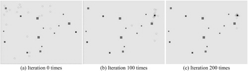
Figure 3. Particles in the iterative process. (a) Iteration 0 times. (b) Iteration 100 times. (c) Iteration 200 times.

There are some parameters in the object function model, which can be adjusted by the user to reflect his emphasis on different factors. In our experiment, these following parameters are set according to experience. Formula (19) represents weights between different factors. And the sum of them should be 1. Formula (20) represents the boundary conditions of different factors. (19) $\begin{array}{rl}{\omega }_Q& =0.35,{\omega }_B=0.25,{\omega }_S=0.25,{\omega }_E=0.15\end{array}$(19) (20) $\begin{array}{rl}{D}_1& =2,D_2=1\end{array}$(20)

The proposed CDQPSO algorithm in this paper was used to solve the above electric business centre location model, which is a 2-dimensional problem. The number of particles was set to 20, each particle is randomly initialized into coordinates, and the number of iterations was set to 200. Algorithm parameters were the same as the previous ones, as listed in Table 2.

4.2. Result analysis

1. The optimization process of the proposed algorithm is shown in Figure 3. Squares of different sizes represent different levels of existing business centres. As can be seen from Figure 3, at the initialization stage, the particles were randomly placed at any position in the candidate region. Along with the iterations process, the particles gradually gathered to the same position. At the 100th iteration, it had basically converged to the final position.

2. Before location optimization, the business average pressure of the business centres in the candidate region was 0.319 according to formula (7), it was 0.290 after the optimization. This indicated that the new business centre effectively relieved the business pressure. Moreover, before and after the optimization process, the values of different kinds of factors considered in the experiment are shown in Table 5. It can be seen that positive factors gradually increased and negative factors gradually decreased. This proved that the CDQPSO algorithm effectively found a location that was more suitable for constructing a business centre.

3. The process of the consumer groups changing in the optimization process is shown in Figures 4 and 5. The larger square represents the existing business centre, and the five-pointed star represents the new-built business centre, and the smaller dots represents consumer groups. Each group randomly which contains 5 to 15 consumers. The dots have the same colour as the square means that these consumers belong to this business centre. From the two figures, we can see that after a new business centre was established, the consumers around it were attracted by it. Therefore, new business centres could effectively relieve the business pressure of existing ones.

4. Finally, to prove the efficiency of the proposed algorithm, the other three popular heuristic algorithms were used to optimize the new business centre position. Also, in the experiment, each algorithm was repeated 15 times to avoid the randomness of the algorithm. From the result comparison given in Table 6, it is obvious that the proposed CDQPSO algorithm obtains the best fitness values among all the algorithm, which proves that the new algorithm has better performance. Through other columns comparison in the table, it is can be found that the position of the business centre can provide consumers with better service and transportation convenience, while keeping the construction cost at a low level.

Figure 4. Consumers before constructing.

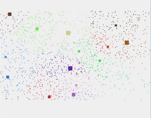
Figure 5. Consumers after constructing.

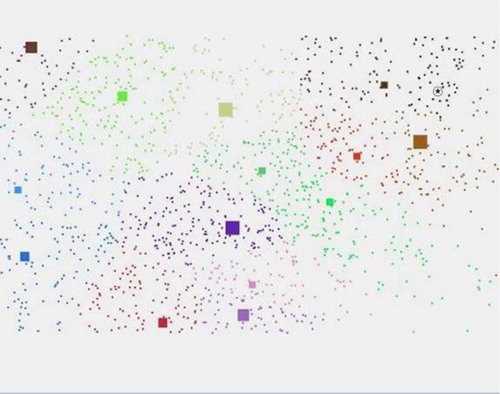
Table 5. Changes of particle factors.

Factors	The first iteration	The last iteration
$Q\left(t\right)$	0.319	0.290
$E\left(t\right)$	1.0	1.0
$B\left(t\right)$	1.0	10.0
$S\left(t\right)$	0.0	5.0
$\text{Fitness}$	0.089	0.033

Table 6. Location result of different algorithms.

Algorithm	Fitness	$Q\left(t\right)$	$E\left(t\right)$	$B\left(t\right)$	$S\left(t\right)$
PSO	0.043	0.294	1.0	8.0	2.0
QPSO	0.043	0.321	1.0	8.0	7.0
CDPSO	0.040	0.292	1.0	10.0	4.0
CDQPSO	0.033	0.290	1.0	10.0	5.0

5. Conclusions

This paper proposes a location model for electric business centre considering positive and negative factors. In order to get an optimal solution for the model, a centre–decentre quantum particle swarm optimization algorithm is proposed by combing the advantage of QPSO and CDPSO Experimental results show that the proposed algorithm has better optimization performance than existing algorithms in standard test functions and real location problem. The new electric business centre location position obtained through our proposed method is more scientific and can bring higher economic and social benefits to the company. In addition, consumers can also obtain higher service ability and transportation convenience.

In our proposed model, the single objective model is implemented by the weighted sum of many factors. However, in the location problem, sometimes multi-objectives should be optimized simultaneously. Therefore, a multi-objective model is our future research work, which is helpful for the decision maker to make trade-off among many objectives more efficiently.

Additional information

Funding

This work was supported in part by the project ‘Research on the Application of the Integration Model Based on IEC-CIM in the Distribution Network and the key Technology of Service Channel’ of State Grid Corporation of China, and the Fundamental Research Funds for the Central Universities [2018ZD06].

Appendix A

References

- Abdelaziz, A. Y., El-Sharkawy, M. A., & Attia, M. A. (2011). Optimal location of thyristor-controlled series compensators in power systems for increasing loadability by genetic algorithm. Electric Power Components and Systems, 39(13), 1373–1387. doi: 10.1080/15325008.2011.584108
- Aras, H., Erdogmus, S., & Koc, E. (2004). Multi-criteria selection for a wind observation station location using analytic hierarchy process. Renewable Energy, 29(8), 1383–1392. doi: 10.1016/j.renene.2003.12.020
- Araz, C., Selim, H., & Ozkarahan, I. (2007). A fuzzy multi-objective covering-based vehicle location model for emergency services. Computers & Operations Research, 34, 705–726. doi: 10.1016/j.cor.2005.03.021
- Bergh, F. V. D. (2006). An Analysis of particle swarm optimizers.
- Bergh, F. V. D, & Engelbrecht, A.P. (2002). A new locally convergent particle swarm optimiser. Proc.of IEEE Int.conf.on Systems Man & Cybernetics, 6. doi: 10.1109/ICSMC.2002.1176018
- Bhaskaran, S., & Turnquist, M. A. (1990). Multiobjective transportation considerations in multiple facility location. Transportation Research, Part A (General), 24(2), 139–148. doi: 10.1016/0191-2607(90)90021-W
- Blanquero, R., & Carrizosa, E. A. D. C. (2002). Biobjective location model. Journal of Global Optimization, 23(2), 139–154. doi: 10.1023/A:1015579208736
- Cabello, H., & Lobillo, F. J. (2016). Sound branch cash management for less: A low-cost forecasting algorithm under uncertain demand. Omega, 70, 118–134. doi: 10.1016/j.omega.2016.09.005
- Chan, F. T. S., & Chung, S. H. (2004). Multi-criteria genetic optimization for distribution network problems. International Journal of Advanced Manufacturing Technology, 24(7–8), 517–532. doi: 10.1007/s00170-002-1445-5
- Colledani, M., & Battaia, O. (2016). A decision support system to manage the quality of end-of-life products in disassembly systems. CIRP Annals-Manufacturing Technology, 65(1), 41–44. doi: 10.1016/j.cirp.2016.04.121
- Cvetkoska, V., & Savic, G. (2017). Efficiency of bank branches: Empirical evidence from a two-phase research approach. Ekonomska Istraživanja/Economic Research, 30, 318–333. doi: 10.1080/1331677X.2017.1305775
- Da, L., Kun, S., & Han, H. (2018). Monthly load forecasting based on economic data by decomposition integration theory. Sustainability, 10, 3282–3304. doi: 10.3390/su10093282
- Diabat, A., Abdallah, T., Al-Refaie, A., Svetinovic, D., & Govindan, K. (2013). Strategic closed-loop facility location problem with carbon market trading. IEEE Transactions on Engineering Management, 60(2), 398–408. doi: 10.1109/TEM.2012.2211105
- Faharani, R. Z., SteadieSeifi, M., & Asgari, N. (2010). Multiple criteria facility location problems: A survey. Applied Mathematical Modeling, 34(7), 1689–1709. doi: 10.1016/j.apm.2009.10.005
- Fernandez, I., & Ruiz, M. C. (2009). Descriptive model and evaluation system to locate sustainable industrial areas. Journal of Cleaner Production, 17(1), 87–100. doi: 10.1016/j.jclepro.2008.02.011
- Ferreira, F., Jalali, M., Ferreira, J., Stankeviciene, J., & Marques, C. (2015). Understanding the dynamics behind bank branch service quality in Portugal: Pursuing a holistic view using fuzzy cognitive mapping. Service Business, 10(3), 469–487. doi: 10.1007/s11628-015-0278-x
- Gomez, M., Jurado, F., Diaz, P., & Ruiz-Reyes, N. (2010). Evaluation of a particle swarm optimization based method for optimal location of photovoltaic grid-connected systems. Electric Power Components and Systems, 38(10), 1123–1138. doi: 10.1080/15325001003652926
- Hakimi, S. L. (1964). Optimum locations of switching centers and the absolute centers and medians of a graph. Operations Research, 12(3), 450–459. doi: 10.1287/opre.12.3.450
- Hsieh, Y. H., Yu, C. C., & Wang, B. F. (2008). Optimal algorithms for the interval location problem with range constraints on length and average. IEEE/ACM Transactions on Computational Biology and Bioinformatics, 5(2), 281–290. doi: 10.1109/TCBB.2007.70217
- Kennedy, J., & Eberhart, R. (1995). Particle swarm optimization. IEEE International Conference on Neural Networks, 1942–1948. doi: 10.1109/ICNN.1995.488968
- Kozanidis, G. (2009). Solving the linear multiple choice knapsack problem with two objectives: Profit and equity. Computational Optimization and Applications, 43(2), 261–294. doi: 10.1007/s10589-007-9140-y
- Kumar, A., & Gao, W. (2009). New price area zonal-based approach for optimal location of distributed generation in hybrid electricity markets. Electric Power Components and Systems, 37(6), 672–692. doi: 10.1080/15325000802705638
- Lin, C. K. Y., & Kwok, R. C. W. (2006). Multi-objective metaheuristics for a location-routing problem with multiple use of vehicles on real data and simulated data. European Journal of Operational Research, 175(3), 1833–1849. doi: 10.1016/j.ejor.2004.10.032
- Quaranta, A. G., Raffoni, A., & Visani, F. (2018). Interfaces with other disciplines a multidimensional approach to measuring bank branch efficiency. European journal of operational research, 266, 746–760. doi: 10.1016/j.ejor.2017.10.009
- Sen, P., Sen, K., & Diwekar, U. M. (2016). A multi-objective optimization approach to optimal sensor location problem in IGCC power plants. Applied Energy, 181, 527–539. doi: 10.1016/j.apenergy.2016.08.006
- Stummer, C., Doerner, K., Focke, A., & Heidenberger, K. (2004). Determining location and size of medical departments in a hospital network: A multiobjective decision support approach. Health Care Management Science, 7(1), 63–71. doi: 10.1023/B:HCMS.0000005399.23600.69
- Sun, J, Xu, W.B, & Feng, B. (2005). A global search strategy of quantum-behaved particle swarm optimization. Proc IEEE Conference on Cybernetics & Intelligent Systems, 111–116. doi: 10.1109/ICCIS.2004.1460396
- Tuzkaya, G., Onut, S., Tuzkaya, U. R., & Gulsun, B. (2008). An analytic network process approach for locating undesirable facilities: An example from Istanbul, Turkey. Journal of Environmental Management, 88(4), 970–983. doi: 10.1016/j.jenvman.2007.05.004
- Villegas, J. G., Palacios, F., & Medaglia, A. L. (2006). Solution methods for the bi-objective (cost-coverage) unconstrained facility location problem with an illustrative example. Annals of Operation Research, 147(1), 109–141. doi: 10.1007/s10479-006-0061-4
- Zhang, Q., Liu, W., Meng, X., Yang, B., & Vasilakos, A. V. (2017). Vector coevolving particle swarm optimization algorithm. Information Sciences, 394, 273–298. doi: 10.1016/j.ins.2017.01.038