Weak fault diagnosis of rolling bearing based on FRFT and DBN

ABSTRACT

When diagnosing the weak fault of rolling bearing, the fault characteristic is difficult to be extracted because the fault signal has a small amplitude and is susceptible to noise. Aiming at this problem, a fault diagnosis method is proposed based on fractional Fourier transform (FRFT) and deep belief networks (DBN). The original fault signal is first transformed into the fractional domain, and the signal is filtered in this domain to extract the fault features. The characteristic signal is then input to the DBN, and the whole network is optimized to finally realized fault diagnosis by using the pre-training and the reverse propagation algorithm. The simulation results show that the method can effectively detect the weak fault of rolling bearing.

KEYWORDS:

• Fault diagnosis
• rolling bearing
• weak fault
• fractional Fourier transform
• deep belief networks

1. Introduction

Rolling bearing has been widely used in rotating machinery due to its high bearing capacity and low friction coefficient, and it is also one of the most vulnerable parts of rotating machinery (Zhong & Huang, 2007). Bearing fault can be divided into significant fault and weak fault according to the evolution process. Weak fault has the characteristics of weak and small amplitude. Due to the harsh working environment, variable working condition and complex environmental structure, the signal has the characteristics of low signal-to-noise ratio, nonlinearity and instability, which make the fault diagnosis very difficult (Abboud, Antoni, Sieg, & Eltabach, 2017; Wen, Lv, Bao, & Liu, 2016). However, any local weak fault may mutate into a significant fault in a short period of time as time passes and propagates, which results in system performance degradation and even leads to major accidents. Effectively eliminating potential safety hazards and reducing economic losses can be achieved by diagnosing bearing faults. Therefore, the weak feature extraction of rolling bearing has been one of the hot topics in the field of bearing fault diagnosis (Zhu, Zhang, & Yuan, 2019).

Recently, some methods have been proposed to extract weak fault characteristics. Short-time Fourier transform (STFT) method (Khodja, Aimer, Boudinar, Benouzza, & Bendiabdellah, 2019; Li, Zhang, Qin, & Sun, 2018) is limited by the window function and has no universality. Wavelet transform method (Guo & Xiao, 2017; Ma, Zhang, Fan, & Wang, 2019; Xu, Tian, Zhang, & Ma, 2019) needs to select an appropriate wavelet base for the fault diagnosis of rolling bearing, and the parameters are pre-set by prior knowledge, where the quality of the parameter selection often has a great impact on the results. The Mahalanobis distance is based on the distribution of features throughout the space as a basis for discrimination, but the sample classification effect is not good under strong noise (Ji, Huang, & Zhou, 2019).

For reducing non-stationary and nonlinear signal noises, empirical mode decomposition (EMD) method (Cheng, Wang, Chen, Zhang, & Huang, 2019; Tao, 2019; Zhang, Zhao, & Deng, 2018) is a common method, but in principle there are problems with modal aliasing and endpoint effects. For noise reduction, singular value decomposition (SVD) method (An, Zeng, Yang, & An, 2017; Cai & Xiao, 2019; Wang et al., 2019) has good performance, but the number of singular values depends on the man-made. If the singular value is too large, it will influence the noise reduction effect. Otherwise, the useful signal will be lost. There is still no valid singular value selection method. Stochastic resonance method (Lei, Qiao, Xu, Lin, & Niu, 2017; Qiao, Lei, Lin, & Jia, 2017) can transfer a part of the noise energy to the signal, while reducing the noise and enhancing the characteristics of the weak signal. However, the traditional adaptive stochastic resonance method has certain limitations because it only has a certain system parameter adjusted and the interactions among parameters are ignored.

Since the weak fault of the rolling bearing has the characteristics of small amplitude, large noise, nonlinearity and instability, the traditional time–frequency analysis method is not applicable. In this paper, the fractional Fourier transform (FRFT) method and the deep belief networks (DBN) method are utilized to deal with this problem. The rolling bearing data can be transformed into the fractional domain by FRFT method, which is more suitable for non-stationary signals. The fault signal will be concentrated in the fractional domain, and the noise reduction filtering can be realized by changing the order of the fractional-order and the noise separation (Ma et al., 2018).

The DBN has a strong ability of feature extraction, and can be used to find distributed features of data by combining low-level features to form abstract high-level features. Therefore, the proposed method inputs the fault signal obtained by FRFT into the DBN, and utilizes the learning and classification capabilities of the DBN to optimize the entire network through error feedback, improves the fault classification result, and realize the fault diagnosis of the rolling bearing. The effectiveness of this method is verified by experimental verification and comparison.

2. Signal pre-processing based on FRFT

2.1. Analysis of FRFT

Compared with the traditional Fourier transform, an angle parameter α is introduced into the FRFT (Ozaktas, Kutayalper, & Zalevsky, 1995), and the p-order FRFT of the signal k(t) is defined as: (1) $K_p\left(u\right)=F^p\left[k\right]\left(u\right)={\int }_{-\mathrm{\infty }}^{+\mathrm{\infty }}{M}_p(t,u)k\left(t\right)dt$(1) where $F^p$ is an operator of the FRFT, $M_p\left(t,u\right)=A_{\alpha }{e}^{\left[j\pi \left(u^{2}cot\alpha -2tucsc\alpha +t^{2}cot\alpha \right)\right]}$ is the kernel function of FRFT, $A_{\alpha }=\sqrt{1-jcot\alpha }$ is the amplitude of FRFT, and $\alpha =p\pi /2$ represents the rotateon angle of the time–frequency plane, p is a fractional-order number.

When $p=4n$, $M_p\left(t,u\right)=\delta \left(u-t\right)$; and when $p=4n+2$, $M_p\left(t,u\right)=\delta \left(u+t\right)$, so that: (2) $M_p\left(t,u\right)=\left\{\begin{array}{ll}{A}_{\alpha }{e}^{\left[j\pi \right(u^{2}cot\alpha -2tucsc\alpha +t^{2}cot\alpha \left)\right]},& \alpha \ne n\pi \\ \delta (t-u),& \alpha =2\text{n}\pi \\ \delta (t+u),& \alpha =(2\text{n}+1)\pi \end{array}\right.$(2) the inverse of FRFT is (3) $k\left(t\right)={\int }_{-\mathrm{\infty }}^{+\mathrm{\infty }}{K}_p\left(u\right)M_{-p}\left(t,u\right)dt$(3)

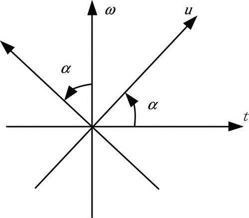
From the formula (3), the signal k(t) can be decomposed into a set of linear combinations of orthogonal LFM bases on the u domain. The u domain is called the fractional Fourier domain. When $p=1$, FRFT is a traditional Fourier transform, so the traditional Fourier transform can be regarded as a special case of FRFT. The physical meaning of Fourier transform can be regarded as the rotation on the time–frequency plane, which rotates the signal 90 degrees counter clockwise from the t axis to the $\omega$ axis, and then FRFT can be represented by the angle of counter clockwise rotation of the signal along the t axis to the $u$ axis, as shown in Figure 1.

Figure 1. Time-frequency plane rotated by an angle.

2.2. FRFT filtering

Since the signal can be decomposed into a linear combination of a set of orthogonal LFM bases on the u domain, the base of the different modulation frequencies can be obtained by changing the angle. Once the chirp signal to be filtered is the same as the modulation frequency of a certain set of fundamental frequencies, the signal is up to an impact function at a set of fundamental frequencies and zero at the other bases.

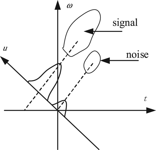
As shown in Figure 2, in the time–frequency distribution diagram, the signal and the noise overlap on the time and the frequency axis, thus the signal and noise cannot be decomposed and filtered. At this time, the signal is rotated around the origin in the time–frequency plane by the FRFT method. When the rotation angle is appropriate, the signal and noise are decomposed in the fractional domain, and then filtered and inversely transformed to extract the signal (Guo, Song, & Zhou, 2012).

Figure 2. Filtering in fractional domain.

In the process, due to the signal has different dimensions in time domain and frequency domain, for the calculation and processing of FRFT, the two intervals $\left[-t_b/2,t_b/2\right]$ and $\left[-f_b/2,f_b/2\right]$ are normalized to $\left[-x_b/2,x_b/2\right]$ and $x_b=(t_b\cdot f_b{)}^{1/2}$. In the actual application process, discrete signal obtained by sampling continuous signal are commonly available. The observation time is $t_0$, and the sampling frequency is $f_s$. Let the time width be the observation time $t_0$, $t_b=t_0$, and take the sampling frequency $f_s$ as the bandwidth fb, $f_b=f_s$, then $x_b=(t_0\cdot f_s{)}^{1/2}$(Zhao, Deng, & Tao, 2005).

2.2. Simulation experiments and analysis

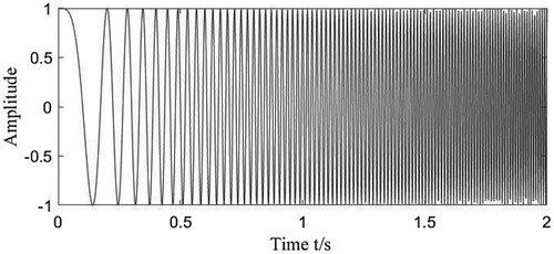
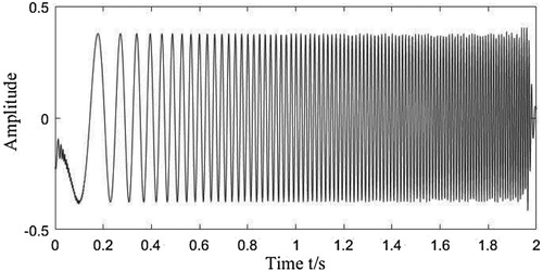
There is a chirp signal, the central frequency is $f_0=100\text{Hz}$, the modulation frequency is $f_m=100\text{Hz}/\text{s}$, the sampling time is $t_0=2\text{s}$, the sampling frequency is $f_s=800\text{Hz}$, and the signal waveform is shown in Figure 3.

Figure 3. Original signal.

A Gaussian white noise with a signal noise ratio of 3 dB is added to the original signal, and the signal waveform with noise is shown in Figure 4.

Figure 4. Signal with noise.

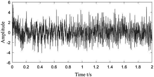
As shown in Figure 4, the original signal is completely submerged in the noise signal. Then, the noisy signal is successively subjected to FRFT in the step of 0.01 in the [1, 1.5] order as shown in Figure 5.

Figure 5. Three-dimensional diagram of signal after fractional Fourier signal.

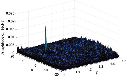
Since $t_0=2\text{s}$ and $f_s=800\text{Hz}$, the normalized fractional domain u has a coordinate range of [−20, 20]. It can be seen from Figure 5 that the peak coordinate of the signal is p = 1.08, u = 2.475, and at 1.08 FRFT order, the signal energy is most concentrated at u = 2.475 in the u domain.

As shown in Figure 6, the signal is bandpass filtered with u = 2.475 at 1.08 FRFT order and then the filtered signal is subjected to the FRFT of p = −1.08. The filtered time-domain signal is shown in Figure 7.

Figure 6. FRFT filtering.

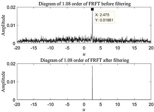
Figure 7. Filtered signal.

It can be seen from Figure 7 that after FRFT filtering, the noise in the original signal is well eliminated. The remaining original signal basically reflects the characteristics of the original signal in addition to the large fluctuation caused by the endpoint effect at the start and end.

3. DBN

A classic deep learning algorithm DBN with powerful feature extraction and learning capabilities (Bengio, 2009) is proposed by Geoffrey Hinton in 2006. It is composed of a number of Restricted Boltzmann machines (RBMs), and unsupervised greedy learning algorithms are used to optimize the connection weights of each layer of RBM.

3.1. RBM model

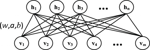
RBM is a generated stochastic neural network with a two-layer cyclic network structure, in which one layer is called the visual layer, that is the input layer, and the other layer is the hidden layer. The nodes in the layer are not connected to each other, and the nodes in the outer layer are connected everywhere. The network structure is shown in Figure 8.

Figure 8. Structure of RBM.

The optimization principle is derived from the classical thermal theory, in which the system is more stable with a smaller energy function. Through training, the network energy is minimized and the optimal parameters of the network are obtained. The energy of the joint configuration of the visible variable v and the implicit variable h is expressed by (4) $E\left(v,h\right)=-\sum _{i=1}^m{a}_i{v}_i-\sum _{j=1}^n{b}_j{h}_j-\sum _{i=1}^m\sum _{j=1}^n{w}_{ij}{v}_i{h}_j$(4) where, v represents the input layer vector, h denotes the hidden layer reconstruction vector and w={w₁₁, … ,w_1n, w₂₁, … ,w_ij, … ,w_nm } stands for the weight between the input layer and the hidden layer. a={a₁, a₂, … , a_m} and b={b₁, b₂, … , b_n} are the offsets of the input layer and the hidden layer, respectively. w_ij represents the weight between the i-th input layer and the j-th hidden layer. v_i and a_i (h_j and b_j) are the state and bias of the i-th input layer (j-th hidden layer), respectively.

The state probability of RBM obeys the regular distribution, and the joint probability distribution of each group (v, h) is (5) $p\left(\mathit{v},\mathit{h}\right)=e^{-E\left(\mathit{v},\mathit{h}\right)}/\phantom{e^{-E\left(\mathit{v},\mathit{h}\right)}\sum _v\sum _h{e}^{-E\left(\mathit{v},\mathit{h}\right)}}\sum _v\sum _h{e}^{-E\left(\mathit{v},\mathit{h}\right)}.$(5) By formula (5), an independent distribution of the input layer vector v can be obtained: (6) $p\left(\mathit{v}\right)=\sum _{h}p\left(\mathit{v},\mathit{h}\right)=\sum _h{e}^{-E\left(\mathit{v},\mathit{h}\right)}/\phantom{\sum _h{e}^{-E\left(\mathit{v},\mathit{h}\right)}\sum _v\sum _h{e}^{-E\left(\mathit{v},\mathit{h}\right)}}\sum _v\sum _h{e}^{-E\left(\mathit{v},\mathit{h}\right)}.$(6)

Since any two units of the same layer of RBM are not connected, according to formula (5), the probabilities of the hidden layer vector h and the input layer vector v can be obtained respectively under the conditions given by the input layer vector v and hidden layer vector h. Considering that the RBM unit is binary with only 0 and 1, under the premise that the activation function is defined as the sigmoid function, the activation probabilities of v and h can be obtained: (7) $\begin{array}{rl}p\left(h_{\text{j}}=1/\mathit{v}\right)& =sigmoid\left(b_j+\sum _{i=1}^m{v}_i{w}_{ij}\right)\end{array}$(7) (8) $\begin{array}{rl}p\left(v_i=1/\mathit{h}\right)& =sigmoid\left(a_i+\sum _{j=1}^n{w}_{ij}{h}_j\right).\end{array}$(8)

According to (7) and (8), if the layer vector v is given, the state of the hidden layer unit h can be calculated by $p\left(h_j=1/\mathit{v}\right)$, and then the state of the reconstructed input layer unit v can be obtained by $p\left(v_i=1/\mathit{h}\right)$. It is known by certain rules that when the difference between the visual layer unit and the reconstructed visual layer unit is minimized, the RBM learning is completed.

3.2. DBN structure

DBN is a ‘black box’ model with multi-layered RBM. In the actual application process, a traditional supervised classifier is added on the top of the RBM to inversely modify the model using samples of known features, and then the data features of the fault samples are matched with the fault types, so that the accuracy of fault diagnosis improved (Lecun, Bengio, & Hinton, 2015). The DBN structure used in this paper is shown in Figure 9.

Figure 9. Schematic diagram of DBN structure.

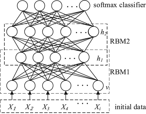
The DBN used herein consists of a 2-layer RBM and a 1-layer Back Propagation (BP) network. In the BP neural network of the last layer, the SoftMax classifier is used to diagnose fault features extracted by the DBN.

4. Fault diagnosis flow based on FRFT and DBN

In this section, the FRFT and DBN are applied to the weak fault diagnosis of rolling bearing. As shown in Figure 10, the specific fault diagnosis process is divided into two parts: the feature extraction part of the original data and the fault diagnosis.

Figure 10. Flow chart of fault diagnosis.

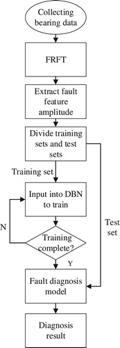
Firstly, the original data are filtered by FRFT to extract the weak fault amplitudes from the original data. Then the extracted fault amplitude is divided into training set and test set through pre-processing. Enter the training set into the DBN network and perform unsupervised training layer by layer between RBM.

After all the RBM training is completed, and then supervised fine-tuning is performed by BP algorithm combined with sample label in the SoftMax classifier. The specific training process is as follows:

Step 1: Parameter initialization. The parameters w, a, b, the learning rate γ are initialized, the reconstruction error ϵ and the number of trainings J are maximized, and the original data are input to the first layer network.

Step 2: Unsupervised training. The greedy algorithm is used to update the parameters w, a, b and check the results. Until the layer RBM reconstruction error is sufficiently small or the number of training runs out, the proceeds to the next layer.

Step 3: Layer-by-layer RBM training. The output of the upper layer of RBM hidden layer is treated as the input of the next layer of RBM input layer. Step 2 is repeated until all RBM training ends.

Step 4: Fine-tune. In the SoftMax classifier, combined with the label of the input sample data, the gradient descent algorithm is used to propagate the error from top to bottom to each layer of RBM, to fine-tune the relevant parameters of the whole DBN.

When the entire network training is completed, the test set sample data are input into the DBN. According to the output results of the network, the fault type of the input test sample can be judged, thereby implementing fault diagnosis.

5. Bearing fault experiment and analysis

5.1. Bearing fault data acquisition

In this paper, the rolling bearing test bench designed and processed by the laboratory is used to generate data.

The test bench comprises a speed regulator, a driving motor, a power box, a rolling bearing mounting frame, an axial loading device and a radial loading device. The speed adjustment range of the test bench speed regulator is 0–3000r/min. The bearings with good condition, spalling on the outer ring, spalling on the inner ring, spalling of the ball and cage break are used in the experiment. The bearing model is 6308, the number of balls Z is 8, the diameter of the steel ball d is 15 mm, the diameter of the raceway E is 65.5 mm, the inner diameter of the bearing is 40 mm, the outer diameter of the bearing is 90 mm, the contact angle a is 0 degree, and the rotation speed is 1309 r/min.

In the experimental, there are 12 samples for each type of data, the frequency of the data is 10240 Hz, and the sampling time is 2 s, so the length of each sample is 20,480. A detailed description of the data is shown in Table 1. The waveform diagram of each type of data is shown in Figures 11–13.

Figure 11. Normal data waveform.

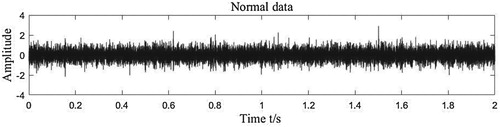
Figure 12. General fault data waveform.

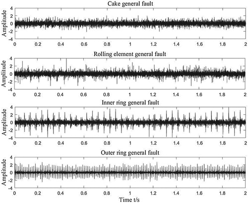
Figure 13. Weak fault data waveform.

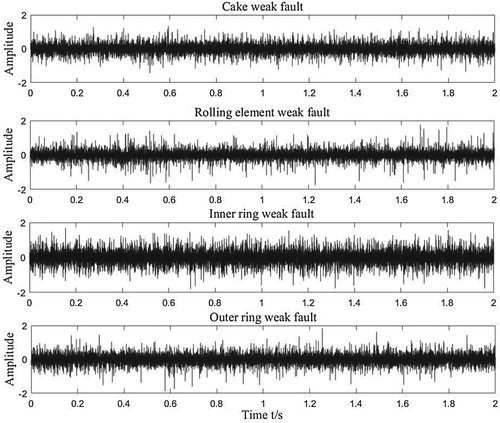
Table 1. Bearing sample data.

Data category	Fault category	Fault description	Fault degree
1	Normal data		Normal
2	Cage break	Cut off	General fault
3	Spalling of the rolling element	About 1 mm^2, in the middle of the raceway
4	Spalling on the inner ring	About 1 mm^2, in the middle of the raceway
5	Spalling on the outer ring	About 1 mm^2, in the middle of the raceway
6	Cage break	1/4 of the cage	Weak fault
7	Spalling of the rolling element	About 0.5 mm^2, slightly deviated
8	Spalling on the inner ring	About 0.5 mm^2, slightly deviated
9	Spalling on the outer ring	About 0.5 mm^2, slightly deviated

As shown in Figures 11–13, in these types of fault, when the bearing has a general failure, the waveforms of inner ring fault and outer ring fault are different from the waveforms of normal data and other general fault, but there is no significant difference between the rolling element, the cage and the normal data waveform. It is difficult to distinguish the fault features of the signal. However, when the bearing has a weak fault, the waveforms of various types of faults are not significantly different and are difficult to be distinguished.

5.2. Fault feature extraction

In this paper, FRFT is used to extract the fault data. Taking the general fault of cage as an example, the general fault of cage is transformed by FRFT. The sampling frequency $f_s\text{is}10240\text{Hz}$, the sampling time $t_0\text{is}2\text{s}$, then $x_b\text{is}-71.6$, and normalized dimension is [−71.6, 71.6]. The three-dimensional diagram of its FRFT is shown in Figure 14.

Figure 14. Three-dimensional diagram of cage fault data FRFT.

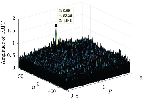
As shown in Figure 14, the signal energy is most concentrated at p = 0.99 steps and u = 52.35. Therefore, the signal is subjected to bandpass filtering at 0.99 FRFT using a peak occlusion method at u = 52.35, and then a −0.99 FRFT variation is performed to obtain a filtered signal. Comparing the waveform of the first second before and after the general fault filter of the cage, the result is shown in Figure 15.

Figure 15. Comparison diagram of cage fault data.

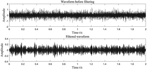
It is obvious that the noise in the filtered signal has been well removed, and the impact characteristics of the fault become more pronounced.

The other types of fault data are FRFT filtered according to the above methods, and the filtered waveforms are shown in Figures 16 and 17.

Figure 16. Other types of general fault filtering waveform.

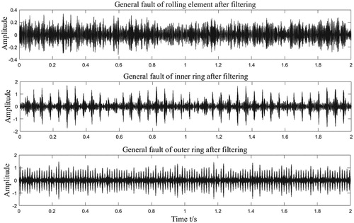
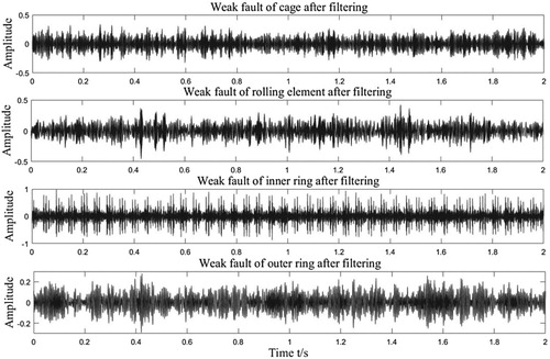
Figure 17. Weak fault filtering waveform.

5.3. DBN bearing fault diagnosis

After the fault data feature is extracted by FRFT, the processed data are input into the DBN to implement fault diagnosis. Since the rotating speed of the bearing is 1309 r/min and the sampling frequency is 10240 Hz, the sampling point of each ring of the bearing is 470 and the length of each long data sample is 20,480. In order to facilitate the calculation, each sample data are divided into 40 short samples, and the length of each short sample is 512. Each type of fault has 12 long data samples, which can be divided into 480 short samples. In those 480 short samples,120 short samples are randomly extracted into a test set and the remaining 360 samples are divided into a training set. Since there are 9 data types in the experiment, the training set and the test set in the DBN have 3240 short samples and 1080 short samples, respectively. The sample labels of 9 types of faults are coded as 100000000, 010000000 … 000000001. In order to understand the feature extraction effect of FRFT on the weak fault of rolling bearing, the extracted fault data are compared with the original fault data in the experiment. Therefore, the original rolling bearing fault data and the FRFT feature extracted data are recorded as data set A and data set B, respectively, as shown in Table 2.

Table 2. Two sample datasets.

Data set	Data category	Training set	Test set	Total
A	Original data	3240	1080	4320
B	FRFT	3240	1080	4320

Because each short sample has a length of 512 and a total of nine sample tags, the input and output layers of the DBN have 512 and 9 cells, respectively. After the experiment, the DBN network hidden layer is set to 2 layers, the hidden layer units are 300 and 100, respectively, the learning rate γ is 0.01, and the number of iterations J is 500.

5.4. Experimental results and analysis

In order to avoid the influence of accidental factors, both dataset A and dataset B are tested 10 times in DBN, and the average correct rate of 9 kinds of faults is shown in Figure 18.

Figure 18. Comparison of accuracy rate of data sets A and B.

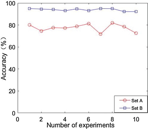
It can be seen from Figure 18 that after the fault feature extraction by FRFT, the fault diagnosis accuracy rate of the rolling bearing is significantly improved.

In data sets A and B, the average accuracy rate of 10 experiments of various types of faults is shown in Table 3.

Table 3. Average diagnosis accuracy rate of each type of fault.

Fault type	Set A (%)	Set B (%)
Normal	100	100
General fault of cage	74.08	91.58
General fault of rolling element	85.50	99.42
General fault of inner ring	91.75	96.50
General fault of outer ring	97.42	93.08
Weak fault of cage	52.83	87.75
Weak fault of rolling element	52.33	95.75
Weak fault of inner ring	85.58	99.41
Weak fault of outer ring	57.33	87.41
Total	77.44	94.5

It can be found from Table 3 that after the feature extraction by FRFT, the accuracy rate of other fault diagnosis is improved remarkably than that of the original data, except the average accuracy rate of the general fault of outer ring is reduced from 97% to 93%. The diagnosis accuracy rate of the general fault of the outer ring is lower because the frequency characteristics of it is more obvious, and the time-domain waveform of the weak fault is similar to the general fault waveform after the FRFT process. Therefore, in the process of diagnosis, a small amount of outer ring general fault is misdiagnosed as a weak fault in the DBN. Before the FRFT processing, the diagnostic accuracy rate for weak faults is only 50%, but after FRFT filtering, the accuracy rate of weak fault diagnosis is increased to 90%. This illustrates the effectiveness of the combination of FRFT and DBN for the diagnosis of weak bearing faults.

6. Conclusion

In this paper, a weak fault diagnosis method has been proposed for rolling bearing based on FRFT and DBN. FRFT has been used to extract fault data which effectively filters out noise signals from the original data and preserves the impact features of the fault signal. The fault is then diagnosed by the powerful classification capability of the DBN method (failure type of rolling bearing). In the simulation experiment, the results of the proposed method have been compared with those of the traditional DBN method. The results have illustrated that the proposed method has higher precision and can greatly improve the accuracy of fault diagnosis.

Disclosure statement

No potential conflict of interest was reported by the author(s).

Additional information

Funding

This work was supported by the National Natural Science Foundation of China [grant number: 61973041].

References

- Abboud, D., Antoni, J., Sieg, Z. S., & Eltabach, M. (2017). Envelope analysis of rotating machine vibrations in variable speed conditions: A comprehensive treatment. Mechanical Systems and Signal Processing, 84, 200–226. doi: 10.1016/j.ymssp.2016.06.033
- An, X. L., Zeng, H. T., Yang, W. W., & An, X. M. (2017). A fault diagnosis of a wind turbine rolling bearing using adaptive local iterative filtering and singular value decomposition. Transactions of the Institute of Measurement and Control, 39(11), 1643–1648. doi: 10.1177/0142331216644041
- Bengio, Y. (2009). Learning deep architectures for AI. Foundations and Trends in Machine Learning, 2(1), 1–127. doi: 10.1561/2200000006
- Cai, J. H., & Xiao, Y. L. (2019). Bearing fault diagnosis method based on the generalized S transform time-frequency spectrum de-noised by singular value decomposition. Proceedings of the Institution of Mechanical Engineers Part C-Journal of Mechanical Engineering Science, 233(7), 2467–3477. doi: 10.1177/0954406218782285
- Cheng, Y., Wang, Z. W., Chen, B. Y., Zhang, W. H., & Huang, G. H. (2019). An improved complementary ensemble empirical mode decomposition with adaptive noise and its application to rolling element bearing fault diagnosis. ISA Transactions, 91, 218–234. doi: 10.1016/j.isatra.2019.01.038
- Guo, B., Song, L. B., & Zhou, G. L. (2012). Application research on fractional Fourier filtering in deception jamming. Acta Electronica Sinica, 40(7), 1328–1332.
- Guo, Y. T., & Xiao, S. Y. (2017). Analysis of rolling bearing fault signal based on wavelet transform. China Measurement & Test, 43(S1), 142–147.
- Ji, H. Q., Huang, K. K., & Zhou, D. H. (2019). Incipient sensor fault isolation based on augmented Mahalanobis distance. Control Engineering Practice, 86, 144–154. doi: 10.1016/j.conengprac.2019.03.013
- Khodja, M. E. A., Aimer, A. F., Boudinar, A. H., Benouzza, N., & Bendiabdellah, A. (2019). Bearing fault diagnosis of a PWM inverter fed-induction motor using an improved short time Fourier transform. Journal of Electrical Engineering & Technology, 14(3), 1201–1210. doi: 10.1007/s42835-019-00096-y
- Lecun, Y., Bengio, Y., & Hinton, G. (2015). Deep learning. Nature, 521, 436–444. doi: 10.1038/nature14539
- Lei, Y. G., Qiao, Z. J., Xu, X. F., Lin, J., & Niu, S. T. (2017). An underdamped stochastic resonance method with stable-state matching for incipient fault diagnosis of rolling element bearings. Mechanical Systems and Signal Processing, 94, 148–164. doi: 10.1016/j.ymssp.2017.02.041
- Li, H., Zhang, Q., Qin, X. R., & Sun, Y. T. (2018). Fault diagnosis method for rolling bearings based on short-time Fourier transform and convolution neural network. Journal of Vibration and Shock, 37(19), 124–131.
- Ma, J. M., Miao, H. X., Su, X. H., Gao, C., Kang, X. J., & Tao, R. (2018). Research progress in theories and applications of the fractional Fourier transform. Opto-Electronic Engineering, 45(6), 170747.
- Ma, P., Zhang, H. L., Fan, W. H., & Wang, C. (2019). Early fault diagnosis of bearing based on frequency band extraction and improved tunable Q-factor wavelet transform. Measurement, 137, 189–202. doi: 10.1016/j.measurement.2019.01.036
- Ozaktas, H. M., Kutayalper, M., & Zalevsky, Z. (1995). The fractional Fourier transform: with applications in optics and signal processing. New York, NJ: Wiley.
- Qiao, Z. J., Lei, Y. G., Lin, J., & Jia, F. (2017). An adaptive unsaturated bistable stochastic resonance method and its application in mechanical fault diagnosis. Mechanical Systems and Signal Processing, 84, 731–746. doi: 10.1016/j.ymssp.2016.08.030
- Tao, X. (2019). Research on fault diagnosis method of rolling bearing based on EMD. Automation & Instrumentation, 34(4), 56–59.
- Wang, F. T., Deng, G., Wang, H. T., Yu, X. G., Han, Q. K., & Li, H. K. (2019). A rolling bearing fault diagnosis method based on EMD and SSAE. Journal of Vibration Engineering, 32(2), 368–376.
- Wen, C. L., Lv, F. Y., Bao, Z. J., & Liu, M. Q. (2016). A review of data driven-based incipient fault diagnosis. Acta Automatica Sinica, 42(9), 1285–1299.
- Xu, Y. G., Tian, W. K., Zhang, K., & Ma, C. Y. (2019). Application of an enhanced fast kurtogram based on empirical wavelet transform for bearing fault diagnosis. Measurement Science and Technology, 30(3), 035001. doi: 10.1088/1361-6501/aafb44
- Zhang, S., Zhao, R. Z., & Deng, L. F. (2018). Weak fault identification of rolling bearings based on VMD singular value entropy. Journal of Vibration and Shock, 37(21), 87–91 + 107.
- Zhao, X. H., Deng, B., & Tao, R. (2005). Dimensional normalization in the digital computation of the fractional Fourier transform. Transactions of Beijing Institute of Technology, 25(4), 360–364.
- Zhong, B. L., & Huang, R. (2007). Mechanical fault diagnosis. BeiJing, BJ: Mechanical fault diagnosis.
- Zhu, Y. S., Zhang, P., & Yuan, Q. Q. (2019). Key technologies and development trend of smart bearing. Journal of Vibration, Measurement & Diagnosis, 39(3), 455–462 + 665.