Zonotope parameter identification for piecewise affine system

ABSTRACT

This paper studies one identification problem for a piecewise affine system which is a special nonlinear system. As the difficulty in identifying the piecewise affine system is to determine each separated region and each unknown parameter vector simultaneously, here we propose a multi-class classification process to determine each separated region. This multi-class classification process is similar to the classical data clustering process, and the merit of our strategy is that the first-order algorithm of convex optimization can be applied to achieve this classification process. Furthermore, to relax the strict probabilistic description on external noise and identify each unknown parameter vector, a zonotope parameter identification algorithm is proposed to compute a set that contains the parameter vector, consistent with the measured output and the given bound of the noise. To guarantee our derived zonotope not growing unbounded with iterations, a sufficient condition for this requirement to hold may be formulated as one linear matrix inequality. Finally, a numerical example confirms our theoretical results.

KEYWORDS:

• Piecewise affine system
• multi-class classification
• zonotope
• parameter identification

1. Introduction

The piecewise affine system considered in this paper is one of the hybrid dynamical systems, as the piecewise affine system represents the switching dynamics among a collection of linear differential or difference equations with state space being partitioned by a finite number of linear hyperplanes. Hybrid dynamical systems are a class of complex systems, which involve interacting discrete events and continuous variable dynamics. They are important in applications in embedded systems, cyber-physical systems, robotics, manufacturing systems, biomolecular networks, and have recently been at the centre of intense research activity in the control theory and artificial intelligence communities. But when to control a system, one needs to know at least something about how the system behaves and reacts to different actions taken on it. Hence, we need a model of the system. A system can be informally defined as an entity which interacts with the rest of the world through more or less well-defined input and output data. A model is then an approximate description of the system, and an ideal model may be simple, accurate and general. This approximate description of the system can be constructed by a system identification strategy, as the goal of system identification is to build a mathematical model for a dynamic system based on some initial information about the system and the measurement data collected from the system. According to (Lennart, 1999), the process of system identification consists in designing and conducting the identification experiment in order to collect the measurement data, selecting the structure of the model and specifying the parameters to be identified and eventually fitting the model parameters to the obtained data. Finally, the quality of the obtained model is evaluated through the model validation process. Generally, system identification is an iterative process and if the quality of the obtained model is not satisfactory, some or all of the listed phases can be repeated in order to obtain one satisfied model for that considered system.

Most commonly used models are linear difference equation descriptions, such as ARX, ARMAX models, and linear state-space models. When linear models are not sufficient for describing accurately the dynamic of a system, a nonlinear model can be employed. A large number of nonlinear model structures have been constructed to investigate their properties, see (Boyd & Vandenberghe, 2004), where some real-time fast convex algorithms are proposed to identify model parameters. Many tools for identification, as well as for control, stability analysis, have emerged in recent years. To be able to use these proposed tools, a mathematical model of the system is needed. Identification of hybrid systems (for example, piecewise affine systems) is an area that is related to many other research fields within nonlinear system identification, as such hybrid systems are sufficiently expressive to model a large number of physical process, and can approximate nonlinear dynamics with arbitrary accuracy. In addition, given the equivalence between piecewise affine systems and several classes of hybrid systems (Pintelon & Schoulens, 2001), piecewise affine system identification techniques can be used to obtain hybrid models. The identification of piecewise affine system is a challenging problem, as it involves the estimation of both the parameters of the affine sub-models and the coefficients of the hyperplanes defining the partition of the state-input set. This issue clearly underlies a classification problem such that each data point corresponds to one sub-model. In particular, one can find several different approaches which are applicable or related to piecewise affine system identification problem. Some examples of approaches for piecewise affine systems are neural networks with piecewise affine perceptions. In (Roll et al., 2004), mixed integer programming is used to solve piecewise affine system identification problem. As the number of integer variables increases with the number of training samples, mixed integer programming is limited to problems with a small number of observations. To be able to reconstruct a possible discontinuous piecewise affine map with a multi-dimensional domain, Giancarlo proposes to exploit the combined use of clustering, linear identification, and pattern recognition techniques, and allows to identify both the affine sub-models and the polyhedral partition of the domain. In (Jouloski & Weiland, 2013) the sub-model parameters are described through probability density functions, which are iteratively updated through particle filtering algorithms. The sum of norms regularization strategy in (Ohlsson & Ljung, 2013) can be computationally heavy in the case of appropriate step size. Piecewise affine system identification problem amounts to learning from a set of training data and the parameters defining each affine sub-model (Lauer et al., 2011). This piecewise affine system identification problem is an NP-hard problem in general, see (Lauer, 2015, 2016), for a detailed explanation of the complexity of piecewise affine system identification. For the sake of simplicity, the sparse property is imposed in piecewise affine systems, then the sparse optimization can greatly improve computational efficiency. The strengths of piecewise affine system identification problem of (Breschi et al., 2016) are the computational efficiency and the ability to be run both in a batch and in a recursive way, where the combined use of recursive multiple least squares and linear multi-category discrimination is chosen for computing a solution of unconstrained optimization problems. When the identification error exists in piecewise affine system is bounded by a quantity, a three-stage procedure of a bounded error approach for parametric identification of piecewise affine autoregressive exogenous models is proposed in (Bemporad & Garulli, 2005). But the performance of that bounded error approach is dependent on noise, overestimated model orders and classification accuracy greatly. The conversion of piecewise affine models from state space input–output form was addressed by deriving necessary and sufficient conditions for a given piecewise affine state-space model to admit equivalent representation (Paoletti & Roll, 2010). From modern control theory, this state-space input–output form can not guaranteed to be a minimal realization, so piecewise affine models are widely used in nonlinear system identification or control. A convex relaxation, based on L1 regulation, is proposed in to approximate the underlying combinatorial problem appearing from piecewise affine regression. The statistical clustering technique in (Nakada & Takaka, 2005) first computes the parameters of the affine local models, then partition of the regressor space. The greedy algorithm of (Paoletti & Jouloski, 2008) to partition in feasible sets of linear inequalities can be computationally heavy in the case of large training sets. The main limitation of the above approach is that the polyhedral partition of the regressor space is given by Voronoi diagram, which will limit flexible capability (Bemporad & Ferrari Trecate, 2000). The problem of finding a lower complexity estimation of piecewise affine models form noise-corrupted input–output data is dealt with in (Giuseppe C Calafiore, 2017), where an identification criterion formed by the average of a standard prediction error cost is combined with an L1 regularization term to promote sparse solution (Xu, 2017). The piecewise linear Hammerstein model can be identified in the presence of a special excitation signal in (Dolanc & Strmcnik, 2005), where it is convenient for the description of the processed with highly nonlinear or discontinuous memoryless static functions. Naoko Miyashita and Yamakita (2007) employs an identification method using pseudo-random binary sequences input for decoupling the identification of nonlinear static block with that of the piecewise affine dynamic block. New iterative algorithms to identify Hammerstein system with piecewise linear nonlinearities are proposed in (Liu & Bai, 2006), further that the normalized iterative method produces a convergent result with smooth nonlinear part and finite impulse linear part. A new form of the Hammerstein model with modified parameterization, which will eliminate the main practical limitations, is introduced in, a parameter estimation algorithm and a novel pole placement controller are presented to tune the identified model. By means of a sparse overparameterization, the identification of nonlinear systems using piecewise linear models is turned into a convex optimization problem in (Mattsson et al., 2016), where a recursive likelihood based on methodology is proposed to penalize model complexity.

As the piecewise affine system is one popular modelling framework for hybrid systems, furthermore piecewise affine system is a special case of switched systems with linear dynamics in each mode and mutual exclusive partitions of the state space. Based on the above descriptions on the piecewise affine system, in this paper, we continue to study the detailed identification strategy for the piecewise affine system. It is well known that in the piecewise affine system, space is partitioned into many separated regions and a local linear form is used for each separated region. So the first step in identifying the piecewise affine system is to determine these separated regions. After the separate regions are given, the second identification problem is reduced to identify the linear sub-models for each region. To deal with the above-mentioned steps, we reformulate the problem of determining the separated regions as a multi-class classification problem, which can be solved by the classical first-order algorithm from convex optimization theory, such as mirror descent algorithm or Nesterov's optimal algorithm. As a multi-class classification problem coincides with a data clustering process into the separated regions. When to identify the unknown parameter in each separated region, many classical identification algorithms can be used directly here, for example, least squares algorithm, maximal likelihood algorithm and Bayesian algorithm. But, all the classical identification algorithms hold in case that the considered noise may be a zero-mean random signal. This condition corresponds to the classical probabilistic description of noise. To relax this strict probabilistic description on noise, we investigate the zonotope parameter identification algorithm in the presence of bounded noise. This bounded noise is considered in the set membership identification field widely, and it is a new deterministic identification algorithm. The zonotope parameter identification algorithm computes a set that contains the parameters, consistent with the measured output and the given bound of the disturbance. To guarantee our derived zonotope not growing unbounded with iterations, some contracting properties can be imposed. In this work, a sufficient condition for these contracting properties to hold may be formulated as one linear matrix inequality. By solving one optimization problem with linear matrix inequality constraint, one approximate feasible solution set is obtained to contain the parameters.

The rest of the paper is organized as follows. In section 2, the problem setting and the piecewise affine system are presented. In section 3, a multi-class classification problem based on the first-order algorithm from convex optimization theory is introduced to determine the separate regions. In section 4, The zonotope parameter identification algorithm is proposed to identify the unknown parameters in the presence of bounded noise for each separated region. In section 5, a very simple numerical example is used to illustrate the proposed algorithm. Finally, conclusions and comments about future research are presented in section 6.

2. Piecewise affine system

Consider an affine model as follows. (1) $y\left(t\right)=-\sum _{i=1}^{n_a}{a}_{i}y(t-i)+\sum _{j=1}^{n_b}{b}_{j}u(t-i)+e\left(t\right)$(1) where $u\left(t\right)$ and $y\left(t\right)$ are input and output respectively, $\left\{a_i\right\}$ and $\left\{b_i\right\}$ are the unknown model parameters, $e\left(t\right)$ is the external noise. Two orders $n_a$ and $n_b$ are known before. This affine model can be rewritten as a linear regression form after a regression vector $\phi \left(t\right)$ is introduced. (2) $\left\{\begin{array}{l}\phi \left(t\right)={\left[\begin{array}{cccccc}-y\left(t-1\right)& \cdots & -y\left(t-n_a\right)& u\left(t-1\right)& \cdots & u\left(t-n_b\right)\end{array}\right]}^T\\ y\left(t\right)={\phi }^T\left(t\right)\theta +e\left(t\right)\end{array}\right.$(2) where the unknown parameter vector is stacked as (3) $\theta ={\left[\begin{array}{cccccc}{a}_1& \cdots & a_{n_a}& b_1& \cdots & b_{n_b}\end{array}\right]}^T$(3) For large enough orders $n_a$ and $n_b$, that affine model can be approximated any linear system. Although affine model (1) is beneficial for the local approximation of some nonlinear systems, it can not capture any nonlinear properties, so in order to introduce the affine model into the nonlinear system, the piecewise affine system is obtained. It means that the parameter vector $\theta$ is dependent on the region in the regression space, where the regression vector $\phi \left(t\right)$ lies. Then the regression space is divided into $n$ separate regions $R_1\cdots R_n$, our considered piecewise affine system can be defined as (4) $y\left(t\right)={\phi }^T\left(t\right){\theta }_i+e\left(t\right)if\phi \left(t\right)\in R_i$(4) where the parameter vector ${\theta }_i$ depends on its separate region $R_i$. The problem of identifying a piecewise affine system is reformulated as that, after output and input $\left\{u\left(t\right),y\left(t\right)\right\}$ are collected, how to identify those unknown parameter vectors $\{{\theta }_i{\}}_{i=1}^n$? Due to the fact that the regression vector $\phi \left(t\right)$ is constituted by output and input $\left\{u\left(t\right),y\left(t\right)\right\}$, so the first step is to judge which region the regression vector belongs to.

3. Multi-class classification process

As there exist $n$ separate regions $R_1\cdots R_n$, the problem of determining which region the regression vector lies is in conjunction with a multi-class classification process. We observe $N$ data points $\{z\left(t\right){\}}_{t=1}^N$. (5) $\begin{array}{rl}z\left(t\right)& ={\left[\begin{array}{cc}y\left(t\right)& \phi \left(t\right)\end{array}\right]}^T\\ & =\left[\begin{array}{ccccc}y\left(t\right)& -y(t-1)& \cdots & -y(t-n_a)& u\left(t-1\right)\end{array}\right.\\ & {\left.\begin{array}{cc}\cdots & u\left(t-n_b\right)\end{array}\right]}^T\end{array}$(5) where $N$ denotes the number of observed data points, and each data point $z\left(t\right)$ belongs to one of $n$ non-overlapping classes, along with labels ${\lambda }_t\in R^n$ which are basic orths in $R^n$; the index of the only non-zero entry in ${\lambda }_t$ is the number of class to which $z\left(t\right)$ belongs. We want to build a multi-class analogy of the standard linear classifier as follows: a multi-class classifier is specified by a matrix $A$ and a vector $a\in R^n$. Given a data point $z\left(t\right)$, we compute the $n$ dimensional vector $Az\left(t\right)+a$, identify its maximal component, and treat the index of this component as our guess for the serial number of the class to which $z\left(t\right)$ belongs.

Let ${\overline{\lambda }}_t=1-{\lambda }_t$ be the component of ${\lambda }_t$. Given a data point $z$ and the corresponding label $\lambda$, let us set. (6) $\begin{array}{rl}h& =h\left(A,a,z,\lambda \right)\\ & =\left[Az+a\right]-\left[\lambda \left(Az+a\right)\right]+\overline{\lambda }\end{array}$(6) If $i_{\ast }$ is the index of the only non-zero entry in $\lambda$, then the $i_{\ast }$ th entry in $h$ is zero. And $h$ is nonpositive if and only if the classifier, given by $A,a$ and evaluated at $z$, recovers the class $i_{\ast }$ of $z$ with margin 1, i.e. we have, (7) $[Az+a{]}_j\le [Az+a{]}_{i_{\ast }}-1\text{for}j\ne i_{\ast }$(7) On the other hand, if the classifier fails to classify $z$ correctly, that is (8) $[Az+a{]}_j\ge [Az+a{]}_{i_{\ast }}\text{for}\text{some}j\ne i_{\ast }$(8) Then the maximal entry in $h$ is $\ge$1. So we set (9) $\eta \left(A,a,z,\lambda \right)=\underset{1\le j\le n}{max}[h\left(A,a,z,\lambda \right){]}_j$(9) We get a non-negative function which vanishes for the pairs $\left(z,\lambda \right)$, which are quite a reliably-with margin $\ge$ 1-classified by $\left(A,a\right)$, and is $\ge$ 1 for the pairs $\left(z,\lambda \right)$ with $z$ not classified correctly. Thus, the function (10) $H\left(A,a\right)=E\left\{\eta \left(A,a,z,\lambda \right)\right\}$(10) The expectation being taken over the distribution of the pairs $\left(z,\lambda \right)$, is an upper bound on the probability for the classifier $\left(A,a\right)$ to misclassify a data point. What we would do is to minimize $H\left(A,a\right)$ over $A$ and $a$. To do this, since $H\left(A,a\right)$ is not observable, we replace the expectation by its empirical counterpart. (11) $H_N\left(A,a\right)=\frac{1}{N}\sum _{t=1}^N\eta \left(A,a,z\left(t\right),{\lambda }_t\right)$(11)

For the sake of simplicity, imposing an upper bound on some norm $||A||$ of $A$, one optimization problem is obtained. (12) $\begin{array}{rl}& \underset{A,a}{min}\frac{1}{N}\sum _{t=1}^N\underset{i\le n}{max}{\left[Az\left(t\right)+a-{\lambda }_t\left(Az\left(t\right)+a\right)+{\overline{\lambda }}_t\right]}_i\\ & \mathrm{s}\mathrm{u}\mathrm{b}\mathrm{j}\mathrm{e}\mathrm{c}\mathrm{t}\mathrm{t}\mathrm{o}||A||\le 1\end{array}$(12) A natural choice of the norm $||A||$ is the maximum of the $||A|{|}_2$ norm. The classical first-order algorithm of convex optimization theory can be used to solve that optimization problem (12), such as mirror descent algorithm or Nesterov's optimal algorithm. Once optimization variables $A$ and $a$ are obtained, then the linear classifier $Az\left(t\right)+a$ is obtained. From the above multi-class classification process, we see that once one data point is collected, we can cluster it with a linear classifier. So based on the above linear classifier, all data points can be clustered together, then those data points clustering together as one class can be used in the second identification problem for one unknown parameter.

4. Zonotope parameter identification algorithm

After all collected data points are clustered as $n$ classes, then those data points belonging to one same class can be used to identify one unknown parameter. Here we only rewrite the following piecewise affine system in the $i$th separate region. (13) $y\left(t\right)={\phi }^T\left(t\right){\theta }_i+e\left(t\right)\phi \left(t\right)\in R_i$(13) The goal of this section is to identify the unknown parameter vector ${\theta }_i$ in the case of the unknown but bounded noise. It is well known that in Equation (13), there are two ways to represent uncertainties: the statistical approach and the deterministic approach. In the statistical approach, the uncertainty or disturbance is modelled by a random process with a known statistical property, it means the probabilistic distribution of the uncertainty or disturbance is available. But in many applications, there are situations when the probabilistic distribution of the uncertainty or disturbance is not known and only bound of the uncertainty can be fixed, then the probabilistic assumptions on the uncertainty are no longer valid. In the deterministic approach, the disturbance is assumed to belong to a set. The main advantage of the deterministic approach is that disturbance is assumed to be unknown but bounded. This is the main reason why we choose the deterministic approach to model the disturbance affecting the system behaviour. Based on this remark, one of the deterministic approach-zonotope parameter identification algorithms has been chosen to identify the unknown parameter vector ${\theta }_i$. This identification algorithm computes a set that contains the parameters consistent with the measured output and the given bound of the disturbance. This set is represented by a zonotope, that is an affine map of a unitary hypercube.

Observing Equation (13) again, as $e\left(t\right)$ represents the considered noise, this noise belongs to a bounded set, i.e. (14) $e\left(t\right)\in \left\{e\in R:|e|\le \sigma \right\}$(14) where $\sigma \in R$ is an upper bound and $e\left(t\right)$ is unknown, but has a known bound.

From set membership identification theory, given a set of measured outputs, the feasible solution set is defined as the set of parameters that are consistent with measured outputs and the given bounds. More precisely, the following definitions are given through this section.

Definition 1

Feasible Solution Set

Suppose that the pairs $\left\{y\left(t\right),\phi \left(t\right)\right\},t=1,2\dots N$ are given. The vector ${\theta }_i$ is said to belong to the feasible solution set if there exists ${\theta }_i$ such that (15) $|y\left(t\right)-{\phi }^T\left(t\right){\theta }_i|\le \sigma ,t=1,2\dots N$(15)

Definition 2

Information set

Given the pairs $\left\{y\left(t\right),\phi \left(t\right)\right\},t=1,2\dots N$ at time instant $t$, the information set $I_t$ is a set of all feasible parameters that are consistent with the model (13), the measured output $y\left(t\right)$ and the known bound at time instant $t$, namely (16) $I_t=\left\{{\theta }_i\in R^{n_a+n_b}:-\sigma \le y\left(t\right)-{\phi }^T\left(t\right){\theta }_i\le \sigma \right\}$(16) Geometrically, $I_t$ represents a strip that is consistent with $\left\{y\left(t\right),\phi \left(t\right)\right\},t=1,2\dots N$. The feasible solution set at time instant $t+1$, denoted as $FS{S}_{t+1}$, can be computed exactly from the one corresponding to time instant $t$ by the following recursion. (17) $FS{S}_{t+1}=FS{S}_t\cap I_t$(17) It is difficult to compute the feasible solution set (Bravo et al., 2016), so an outer bound of the feasible solution set can be used.

Definition 3

Approximated Feasible Solution Set

An approximated feasible solution set denoted AFSS, is a set that satisfies that FSS. The intersection $FS{S}_t\cap I_t$ is approximated by means of the intersection between a zonotope and a strip at a time instant $t$.

Definition 4

Zonotope of order $m$

Given a vector $p\in R^{n_a+n_b}$ and a matrix $H\in R^{\left(n_a+n_b\right)\times m}$, a zonotope of order $m$ is a set of $n_1=n_a+n_b$ dimensional vectors defined by. (18) $Z=\left\{{\theta }_i\in R^{n_1}:{\theta }_i\in p\oplus H{B}^m\right\}$(18) where $H{B}^m$ is a linear projection of $B^m$ into $n_1=n_a+n_b$ dimensional parameter space, $B^m$ is a unit hypercube of order $m$, and $\oplus$ denotes Minkowski sum.

Using the approximated feasible solution set on the intersection (17), then (19) $FS{S}_{t+1}=FS{S}_t\cap I_t\subseteq AFS{S}_{t+1}$(19) If in Equation (19) a feasible solution set $FS{S}_t$ is denoted by a zonotope and information set $I_t$ is a strip, then a family of zonotopes, which over-bound the intersection between a zonotope and a strip, are derived as the following Theorem 1.

Theorem 1:

Suppose FSS at time instant $t$, denoted as a zonotope (20) $FS{S}_t={\hat{p}}_t\oplus {\hat{H}}_t{B}^r\subset R^{n_1}$(20) The information set or a strip (21) $I_t=\left\{{\theta }_i\in R^{n_a+n_b}:-\sigma \le y\left(t\right)-{\phi }^T\left(t\right){\theta }_i\le \sigma \right\}$(21) and a scalar $\gamma$, define (22) $\left\{\begin{array}{l}{\hat{p}}_t\left(\gamma \right)={\hat{p}}_t+\gamma \left(y\left(t\right)-{\phi }^T\left(t\right){\hat{p}}_t\right)\\ {\hat{H}}_t\left(\gamma \right)=\left[\begin{array}{cc}\left(I-\gamma \phi \left(t\right)\right){\hat{H}}_t& \sigma \gamma \end{array}\right]\end{array}\right.$(22) Thus, we have (23) $\begin{array}{rl}FS{S}_{t+1}& =FS{S}_t\cap I_t\subseteq AFS{S}_{t+1}\\ & ={\hat{p}}_t\left(\gamma \right)\oplus {\hat{H}}_t\left(\gamma \right)B^{r+1}\end{array}$(23) where $I$ is an identity matrix.

The optimization-based method is used to choose a scalar $\gamma \in R$, by minimizing the volume of a zonotope. Now the minimization of the P-radius of a zonotope is applied, as the P-radius criterion allows to guarantee the non-increasing property of the guaranteed zonotope at each time instant/. It tells us that to guarantee the approximated feasible solution set not growing unbounded with iteration steps, the following inequality relation between two neighbouring zonotopes is imposed. (24) $l_t\le \text{β}{l}_{t-1}+{\sigma }^2$(24) where $\text{β}\in \left(0,1\right]$ is a contraction rate, and $l_t$ is the P-radius of zonotope parameter estimation set at time instant $t$, which is defined by (25) $l_t=\underset{{\theta }_i\in FS{S}_t}{max}\left(||{\theta }_i-{\hat{p}}_t|{|}_P^2\right)$(25) where $P$ is an $n_1$-dimensional positive definite matrix.

Substituting the definition (25) into the inequality relation (24), we have (26) $\begin{array}{r}\underset{\hat{z}\in B^{r+1}}{max}\left(||{\hat{H}}_t\left(\gamma \right)\hat{z}|{|}_P^2\right)\le \underset{z\in B^r}{max}\text{β}\left(||{\hat{H}}_{t-1}z|{|}_P^2\right)+\underset{\eta \in B^1}{max}||\sigma \eta |{|}_2^2\end{array}$(26) Expanding Equation (26) to obtain (27) ${\hat{z}}^T{\hat{H}}_t\left(\gamma \right)P{\hat{H}}_t\left(\gamma \right)\hat{z}-\text{β}{z}^T{\hat{H}}_{t-1}P{\hat{H}}_{t-1}z-{\eta }^2{\sigma }^2\le 0$(27)

Due to the recursion of ${\hat{H}}_t\left(\gamma \right)$ in Equation (22), we compute. (28) $\begin{array}{rl}{\hat{H}}_t\left(\gamma \right)\hat{z}& =\left(I-\gamma \phi \left(t\right)\right){\hat{H}}_{t-1}z+\sigma \gamma \eta \\ & =\left(I-\gamma \phi \left(t\right)\right)\overline{z}+\sigma \gamma \eta \end{array}$(28) where we set (29) $\left\{\begin{array}{l}\overline{z}={\hat{H}}_{t-1}z\\ \hat{z}={\left[\begin{array}{cc}z& \eta \end{array}\right]}^T\end{array}\right.$(29)

Applying Equation (28) in Equation (27), we obtain. (30) $\begin{array}{rl}& \left[{\overline{z}}^T{\left(I-\gamma \phi \left(t\right)\right)}^T+\sigma \gamma \eta \right]P\left[\left(I-\gamma \phi \left(t\right)\right)\overline{z}+\sigma \gamma \eta \right]\\ & -\text{β}{\overline{z}}^{T}P\overline{z}-{\eta }^2{\sigma }^2\le 0\end{array}$(30) Formulating above inequality as (31) $\begin{array}{r}{\overline{z}}^T(I-\gamma \phi \left(t\right){)}^{T}P\left(I-\gamma \phi \left(t\right)\right)\overline{z}+{\overline{z}}^T(I-\gamma \phi \left(t\right){)}^{T}P\sigma \gamma \eta \\ +\sigma \gamma \eta P\left(I-\gamma \phi \left(t\right)\right)\overline{z}+{\sigma }^2{\gamma }^2{\eta }^2-\text{β}{\overline{z}}^{T}P\overline{z}-{\eta }^2{\sigma }^2\le 0\end{array}$(31)

A sufficient condition for Equation (31) to hold can be rewritten as one linear matrix inequality. (32) $\begin{array}{rl}& {\left[\begin{array}{c}\overline{z}\\ \eta \end{array}\right]}^T\left[\begin{array}{cc}{\left(I-\gamma \phi \left(t\right)\right)}^{T}P\left(I-\gamma \phi \left(t\right)\right)-\text{β}P& {\left(I-\gamma \phi \left(t\right)\right)}^{T}P\sigma \gamma \\ P\sigma \gamma \left(I-\gamma \phi \left(t\right)\right)& {\sigma }^2\left({\gamma }^2-1\right)\end{array}\right]\\ & \left[\begin{array}{c}\overline{z}\\ \eta \end{array}\right]\le 0,\mathrm{\forall }\overline{z},\eta \end{array}$(32) Using the definition of positive definite matrix allows us to rewrite as follows. (33) $\begin{array}{rl}& \left[\begin{array}{cc}{\left(I-\gamma \phi \left(t\right)\right)}^{T}P\left(I-\gamma \phi \left(t\right)\right)-\text{β}P& {\left(I-\gamma \phi \left(t\right)\right)}^{T}P\sigma \gamma \\ P\sigma \gamma \left(I-\gamma \phi \left(t\right)\right)& {\sigma }^2\left({\gamma }^2-1\right)\end{array}\right]\\ & \le 0\mathrm{\forall }\left[\begin{array}{c}\overline{z}\\ \eta \end{array}\right]\ne 0\end{array}$(33)

The linear matrix inequality in (33) defines the feasible solution for scalar $\gamma$, i.e. $\gamma$ can be computed by solving the following Eigenvalue problem. (34) $\begin{array}{rl}& \underset{\tau ,\gamma }{max}\tau \\ & \text{subject to}\frac{\left(1-\text{β}\right)P}{\underset{\eta \in B}{max||\gamma \eta |{|}_2^2}}\ge \tau I,\tau >0\\ & \left[\begin{array}{cc}{\left(I-\gamma \phi \left(t\right)\right)}^{T}P\left(I-\gamma \phi \left(t\right)\right)-\text{β}P& {\left(I-\gamma \phi \left(t\right)\right)}^{T}P\sigma \gamma \\ P\sigma \gamma \left(I-\gamma \phi \left(t\right)\right)& {\sigma }^2\left({\gamma }^2-1\right)\end{array}\right]\le 0\end{array}$(34) The above Eigenvalue problem can be solved by using the convex optimization algorithm, then based on this optimal scalar $\gamma \in R$, a zonotopic outer approximation of the intersection between a zonotope and a strip is obtained by using the matrix inequality optimization strategy.

Algorithm 1

Zonotope Parameter Identification Algorithm

1. Obtain measured input–output data and construct a regressor vector $\phi \left(t\right)$;

2. Build a strip that bounds the consistent parameters, i.e. information set; $I_t=\left\{{\theta }_i\in R^{n_a+n_b}:-\sigma \le y\left(t\right)-{\phi }^T\left(t\right){\theta }_i\le \sigma \right\}$

3. Construct a zonotope $FS{S}_t={\hat{p}}_t\oplus {\hat{H}}_t{B}^r\subset R^{n_1}$ to denote the feasible solution set at time instant $t$;

4. Compute the intersection between a zonotope and a strip at time instant $t$ and obtain a new zonotope $\begin{array}{cc}FS{S}_{t+1}& =FS{S}_t\cap I_t\subseteq AFS{S}_{t+1}\\ & ={\hat{p}}_t\left(\gamma \right)\oplus {\hat{H}}_t\left(\gamma \right)B^{r+1}\end{array}$

to denote the approximated feasible solution set at time instant $t+1$;

1. Choose one optimal scalar $\gamma$ by solving one matrix inequality optimization strategy;

2. Repeat the above steps and terminate the recursive algorithm when the P-radius $l_t$is zero, then denote ${\hat{p}}^{\ast }$ as the vector in the last zonotope, so the unknown parameter vector ${\theta }_i$ is given by (35) ${\hat{\theta }}_i={\hat{p}}^{\ast }$(35)

It is similar to applying the above six steps to identify another unknown parameter vector.

Comment: Based on the linear matrix inequality (24), it corresponds to the contracting properties between two neighbouring zonotopes, then this linear matrix inequality can be regarded as one sufficient condition to guarantee that the volume of the obtained zonotope will be decreased with the iteration step increase. It means that after the above six steps are stopped, the volume of the final zonotope will be sufficiently small, then the centre of the final zonotope can be chosen as the parameter estimation. So the convergence consistency of our proposed zonotope parameter identification algorithm can be guaranteed by the added contracting properties.

5. Numerical example

In this section, one simple piecewise affine system is used to prove our strategies, such as two-class classification process and zonotope parameter identification algorithm. This simple piecewise affine system is given as follows. (36) $y\left(t\right)=\left\{\begin{array}{l}{\phi }^T\left(t\right){\theta }_1+e\left(t\right)\mathrm{i}\mathrm{f}\phi \left(t\right)>0\\ {\phi }^T\left(t\right){\theta }_2+e\left(t\right)\mathrm{i}\mathrm{f}\phi \left(t\right)\le 0\end{array}\right.$(36) where the condition that the regression vector $\phi \left(t\right)$ satisfies $\phi \left(t\right)>0$ means all the elements in regression vector $\phi \left(t\right)$ are positive. Also, the condition that the regression vector $\phi \left(t\right)$ satisfies $\phi \left(t\right)\le 0$ means all the elements in regression vector $\phi \left(t\right)$ are negative or zero.

The regression vector $\phi \left(t\right)$ and two unknown parameter vectors $\left({\theta }_1,{\theta }_2\right)$ are described as (37) $\left\{\begin{array}{l}\phi \left(t\right)={\left[\begin{array}{cc}-y\left(t\right)& -u\left(t\right)\end{array}\right]}^T\\ {\theta }_1={\left[\begin{array}{cc}7& 2\end{array}\right]}^T\\ {\theta }_2={\left[\begin{array}{cc}2& 0.5\end{array}\right]}^T\end{array}\right.$(37) We exert the input signal $u\left(t\right)$ in the piecewise affine system. The actual input signal is given in Figure 1(a), but this actual input signal is not suited for simulation. So we use its approximated input signal to replace the actual input signal in our simulation, where the approximated input signal is similar to sinusoidal signal-Figure 1(b). 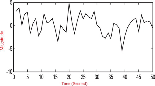Then we measure the output signal $y\left(t\right)$ by using some measuring devices, the observed output signal is plotted in Figure 2.

Figure 1. The applied input signal. (a) Actual input signal. (b) Approximated input signal.

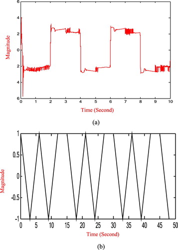
Figure 2. The observed output signal.

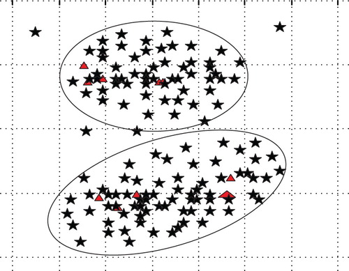
Firstly our mentioned multi-class classification process is reduced to two-class classification problem. Given one data point $\left(y\left(t\right),\phi \left(t\right)\right)$, we determine which region this data point belongs to. Here the number of given data points is $N=500$, i.e. these 500 data points belong to one of two classes. The clustering process can be seen in Figure 3, where data points are clustered around two ellipsoids. As three points deviate away these two ellipsoids, then they are regarded as outliers and we delete them. From Figure 3, all data points are classified correctly, except three data points.

Figure 3. The observed output signal.

Secondly in the presence of bounded noise, choose upper bound $|e\left(t\right)|\le \sigma =0.5$and all initial parameter values are chosen as ${\hat{\theta }}_0=\frac{1}{p_0}I$

The zonotope parameter identification algorithm is applied to identify those two unknown parameter vectors. Applying above six steps to construct a sequence of candidate zonotopes, and after 20 iterations, these candidate zonotopes are given in Figures 4 and 5.

Figure 4. The observed output signal.

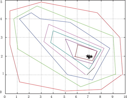
Figure 5. The observed output signal.

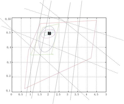
In Figure 4, the black star denotes the optimal parameter vector as ${\theta }_1={\left[\begin{array}{cc}7& 2\end{array}\right]}^T$, and a sequence of candidate zonotopes generated by the zonotope parameter identification algorithm include ${\theta }_1={\left[\begin{array}{cc}7& 2\end{array}\right]}^T$ as their interior points. As the volumes of these candidate zonotopes decreased with iterations, i.e. certain contracting properties hold. Generally, the other unknown parameter vector corresponding to ${\theta }_1={\left[\begin{array}{cc}7& 2\end{array}\right]}^T$ can be chosen as the centre of the smallest zonotope. Furthermore, the black star is the optimal parameter vector as ${\theta }_2={\left[\begin{array}{cc}2& 0.5\end{array}\right]}^T$ in Figure 5, and results are similar to them in Figure 4.

From Figure 3, all data points are classified correctly, so Figure 3 can be used to measure the performance of the multi-class classification process.

Figures 4 and 5 are used to measure the performance of the zonotope parameter identification algorithm, the black star is the optimal parameter vector. After running the zonotope parameter identification algorithm, one sequence of zonotopes are obtained. And the optimal parameter vector is an interior point or a centre of the smallest zonotope.

6. Conclusion

In this paper, we study the problem of identifying the piecewise affine system, which combines the linear and nonlinear property. As it is piecewise affine in the regression space, the parameter vector depends on the region in the regression space. The separated regions are determined as a multi-class classification problem, which is solved by the classical first-order algorithm from convex optimization theory. In the presence of unknown but bounded noise, zonotope parameter identification algorithm is proposed to identify unknown parameter vector in each separated region. Generally, finite sample property of the zonotope parameter identification algorithm is our ongoing work.

Acknowledgements

The authors are grateful to Professor Eduardo F Camacho for his warm invitation in his control lab at the University of Seville, Seville, Spain. The authors thank for his assistance and advice on zonotopes in guaranteed state estimation and model predictive control.

Disclosure statement

No potential conflict of interest was reported by the author(s).

Additional information

Funding

This work was supported by the Grants from the National Science Foundation of China [grant number 61364014].

References

- Bemporad, A., & Ferrari Trecate, G. (2000). Observability and controllability of piecewise affine and hybrid systems. IEEE Transactions on Automatic Control, 45(10), 1864–1876. https://doi.org/10.1109/TAC.2000.880987
- Bemporad, A., & Garulli, A. (2005). A bounded error approach to piecewise affine system identification. IEEE Transactions on Automatic Control, 50(10), 1567–1580. https://doi.org/10.1109/TAC.2005.856667
- Boyd, S., & Vandenberghe, L. (2004). Convex optimization. Cambridge University Press.
- Bravo, J. M., Suarez, A., Vasallo, M., & Alamo, T. (2016). Slide window bounded error time varying system identification. IEEE Transactions on Automatic Control, 61(8), 2282–2287. https://doi.org/10.1109/TAC.2015.2491539
- Breschi, V., Piga, D., & Bemporad, A. (2016). Piecewise affine regression via recursive multiple least squares and multi-category discrimination. Automatica, 73(11), 155–162. https://doi.org/10.1016/j.automatica.2016.07.016
- Calafiore, G. C. (2017). Leading impulse response identification via the elastic net criterion. Automatica, 80(4), 75–87. https://doi.org/10.1016/j.automatica.2017.01.011
- Dolanc, G., & Strmcnik, S. (2005). Identification of nonlinear systems using a piecewise-linear Hammerstein model. Systems & Control Letters, 54(2), 145–158. https://doi.org/10.1016/j.sysconle.2004.08.002
- Jouloski, A. L., & Weiland, S. (2013). A Bayesian approach to identification of hybrid systems. IEEE Transactions on Automatic Control, 50(10), 1520–1533. https://doi.org/10.1109/TAC.2005.856649
- Lauer, F. (2015). On the complexity of piecewise affine system identification. Automatica, 62(12), 148–153. https://doi.org/10.1016/j.automatica.2015.09.031
- Lauer, F. (2016). On the complexity of switching linear regression. Automatica, 74(12), 80–83. https://doi.org/10.1016/j.automatica.2016.07.027
- Lauer, F., Bloch, G., & Vidal, R. (2011). A continuous optimization framework for hybrid system identification. Automatica, 47(3), 608–613. https://doi.org/10.1016/j.automatica.2011.01.020
- Lennart, L. (1999). System identification: Theory for the user. Prentice Hall Press.
- Liu, Y., & Bai, E.-W. (2006, June 14–16). Iterative identification of Hammerstein systems with piecewise-linear nonlinearities. Proceedings of the 2006 American control Conference, Minneapolis, Minnesota, USA.
- Mattsson, P., Zachariah, D., & Stoica, P. (2016). Recursive identification method for piecewise ARX models: A sparse estimation approach. IEEE Transactions on Signal Processing, 64(19), 5082–5093. https://doi.org/10.1109/TSP.2016.2595487
- Miyashita, N., & Yamakita, M. (2007, July 11–13). Identification of Hammerstein systems with piecewise-affine nonlinearities. Proceedings of the 2007 American control conference, New York, USA.
- Nakada, H., & Takaka, K. (2005). Identification of piecewise affine systems based on statistical clustering technique. Automatica, 41(5), 905–913. https://doi.org/10.1016/j.automatica.2004.12.005
- Ohlsson, H., & Ljung, L. (2013). Identification of switched linear regression models using sum of norms regularization. Automatica, 49(4), 1045–1050. https://doi.org/10.1016/j.automatica.2013.01.031
- Paoletti, S., & Jouloski, A. L. (2008). Identification of hybrid systems a tutorial. European Journal of Control, 13(2), 242–260. https://doi.org/10.3166/ejc.13.242-260
- Paoletti, S., & Roll, J. (2010). On the input output representation of piecewise affine state space models. IEEE Transactions on Automatic Control, 55(1), 60–72. https://doi.org/10.1109/TAC.2009.2034224
- Pintelon, R., & Schoulens, J. (2001). System identification: A frequency domain approach. IEEE Press.
- Roll, J., Bemporad, A., & Ljung, L. (2004). Identification of piecewise affine systems via mixed integer programming. Automatica, 40(1), 37–50. https://doi.org/10.1016/j.automatica.2003.08.006
- Xu, X. (2017). Distributed emitter parameter refinement based on maximum likelihood. International Journal of Intelligent Computing and Cybernetics, 10(1), 2–11. https://doi.org/10.1108/IJICC-11-2015-0035