The 2-good-neighbour diagnosability of modified bubble-sort graphs under the PMC and MM* model

Abstract

The study of interconnection networks is a hot topic for multiprocessor systems. Diagnosability plays an important role in the study of interconnection networks. A new measure for fault diagnosis of a system is proposed by Peng et al. in 2012. It is called g-good-neighbour diagnosability which restrains every fault-free vertex containing at least g fault-free neighbours. The n-dimensional modified bubble-sort graph $M{B}_n$ is a special Cayley graph. In this paper, we give that the 2-good-neighbour diagnosability of $M{B}_n$ under the PMC model is 4n−5 for $n\ge 4$ and the 2-good-neighbour diagnosability of $M{B}_n$ under the $M{M}^{\ast }$ model is 4n−5 for $n\ge 4$.

Keywords:

• Interconnection network
• diagnosability
• modified bubble-sort graph
• 2-good-neighbour

1. Introduction

A multiprocessor system is modelled as an undirected graph $G=(V,E)$, whose vertices represent processors and edges represent communication links. Some of the vertices in G may fail when the system is put into use, so identify faulty vertices is crucial for reliable computing. The process of identifying faulty vertices is called the diagnosis of the system. A system is said to be t-diagnosable if all faulty processors can be identified without replacement, provided that the number of faults presented does not exceed t. The diagnosability $t\left(G\right)$ of a system G is the maximum value of t such that G is t-diagnosable (Dahbura & Masson, 1984; Fan, 2002; Lai et al., 2005).

For the purpose of diagnosing of a system, a number of models have been proposed. Among these models, the most popular is the PMC model proposed by Preparata et al. (1967). The PMC model assumed that each vertex can test its neighbouring vertices, and the test results are ‘faulty’ and ‘fault-free’. Under this model, each vertex $u\in V\left(G\right)$ is able to test another vertex $v\in V\left(G\right)$ if $uv\in E\left(G\right)$, where u is called the tester and v is called the tested vertex. If the tested vertex v is faulty, the result of the test $(u,v)$ is 1. The outcome of a test performed by a faulty tester is unreliable. Usually, we assume that the testing result is reliable. A test assignment T is the collection of tests for each adjacent pair of vertices in G. And T can be modelled as a directed testing graph $T=\left(V\right(G),L)$, where $(u,v)\in L$ implies that u is adjacent to v in G. The collection of all test results for a test assignment T is called a syndrome, denoted by σ. If the vertices in $F\subseteq V\left(G\right)$ are all faulty, F is called a faulty set of G. For any $(u,v)\in L$ and a subset of vertices $F\subseteq V\left(G\right)$, a syndrome σ is given by $u\in V\mathrm{\setminus }F$, $\sigma (u,v)=1$ if and only if $v\in L$, then F is said to be consistent with σ. Then F is a possible set of faulty vertices. Different faulty sets may produce the same syndrome. We use $\sigma \left(F\right)$ to represent the set of all syndromes which could be produced on the condition of F is the set of faulty vertices. Two distinct sets $F_1$ and $F_2$ in $V\left(G\right)$ are said to be indistinguishable if $\sigma \left(F_1\right)\cap \sigma \left(F_2\right)\ne \mathrm{\varnothing }$, otherwise, $F_1$ and $F_2$ are said to be distinguishable. Besides, $(F_1,F_2)$ is an indistinguishable pair if $\sigma \left(F_1\right)\cap \sigma \left(F_2\right)\ne \mathrm{\varnothing }$; else, $(F_1,F_2)$ is a distinguishable pair.

To grant more accurate diagnosis for a large-scale system, Lai et al. (2005) introduced the conditional diagnosability of a system under the PMC model, they considered the situation that any fault set cannot contain all the neighbours of any vertex in the system. Another major approach is the comparison diagnosis model (MM model) which was proposed by Maeng and Malek (1981). In order to diagnose the system under the MM model, a vertex sends the same task to two of its neighbours and compares their responses. It is same as the PMC model, the output of a comparison performed by a faulty vertex is unreliable. So we assume the output is reliable. The comparison scheme of a system G is modelled as $M\left(V\right(G),L)$, which is a multi-graph and L is the labelled-edge set. A labelled-edge $(u,v{)}_w\in L$ represents a comparison which two vertices u and v are compared by a vertex w; and it implies $uw,vw\in E\left(G\right)$. The collection of all comparative results in $M\left(V\right(G),L)$ is called the syndrome of the diagnosis, it is denoted by ${\sigma }^{\ast }$. ${\sigma }^{\ast }(u,v{)}_w=1$, if the comparison $(u,v{)}_w$ disagrees; otherwise, ${\sigma }^{\ast }(u,v{)}_w=0$. The $M{M}^{\ast }$ model (Dahbura & Masson, 1984) is a special case of the MM model. In the $M{M}^{\ast }$ model, all comparisons of G are in the comparison scheme of G, i.e. if $uw,vw\in E\left(G\right)$, then $(u,v{)}_w\in L$. The same as the PMC model, we can define two distinct subsets of vertices $F_1$ and $F_2$ in $V\left(G\right)$ which are consistent with a given syndrome ${\sigma }^{\ast }$ and the sets $F_1$ and $F_2$ are indistinguishable (resp. distinguishable) under the $M{M}^{\ast }$ model. A new measure for faulty diagnosis of G was proposed by Peng et al. (2012), this measure requires fault-free vertex has at least g fault-free neighbours. It was called the g-good-neighbour diagnosability. For a given system $G=(V,E)$, $F_1$ and $F_2$ are two distinct g-good-neighbour faulty subsets of G, with $|F_1|\le t$, $|F_2|\le t$, G is called g-good-neighbour t-diagnosable if and only if $F_1$ and $F_2$ are distinguishable for any distinct pair of $(F_1,F_2)$. The g-good-neighbour diagnosability $t_g\left(G\right)$ of G is the maximum value of t such that G is g-good-neighbour t-diagnosable. The diagnosability of systems has received much attention, for details, see Wang and Han (2016), Wang et al. (2017) and Wang et al. (2016).

The modified bubble-sort graph has been proved to be an important viable candidate for interconnecting a multiprocessor system (Akers & Krishanmurthy, 1989; Lakshmivarahan et al., 1993; Yu & Huang, 2012). Yu et al. (2013) showed that the 2-good-neighbour connectivity of modified bubble-sort graphs was 4n−8 for $n\ge 4$. Cheng and Lipták (2007) proved that the 1-good-neighbour connectivity of modified bubble-sort graphs was 2n−2. Wang et al. (2017) studied the 2-good-neighbour diagnosability of the bubble-sort star graph $B{S}_n$, and Wang et al. (2016) studied the 2-good-neighbour diagnosability of a class of Cayley graph $C{\mathrm{\Gamma }}_n$. We had proved that the 3-good-neighbour connectivity of modified bubble-sort graphs was 8n−24 for $n\ge 6$ (Wang & Wang). We also proved that the 3-good-neighbour diagnosability of modified bubble-sort graphs under the PMC model and $M{M}^{\ast }$ model (Wang & Wang), respectively. In this paper, we evaluate the 2-good-neighbour diagnosability of modified bubble-sort graphs under the PMC model and $M{M}^{\ast }$ model, respectively.

2. Preliminaries

In this section, we will give some definitions and notations which are needed for our discussion.

2.1. Definitions and notations

Let $G=(V,E)$ be an undirected simple graph and $S\subseteq V\left(G\right)$ be a nonempty vertex subset of G. The induced subgraph $G\left[S\right]$ is the graph whose vertex set is S and the edge set is the set of all the edges of G with both endpoints in S. The degree $d_G\left(v\right)$ of a vertex is the number of edges incident to the vertex, with loops counted twice. The minimum degree of vertices in G is denote by $\delta \left(G\right)$. For any vertex v, $N_G\left(v\right)$ is the neighbourhood of v in G which is the set of vertices adjacent to v. u is called a neighbour vertex of v when $u\in N_G\left(v\right)$. We use $N_G\left(S\right)$ to denote the set ${\cup }_{v\in S}{N}_G\left(v\right)\mathrm{\setminus }S$. A vertex cut of a connected graph G is a set of vertices whose removal renders G disconnected. The vertex connectivity $\kappa \left(G\right)$ is the size of a minimal vertex cut. A closed trail whose origin and internal vertices are distinct is a cycle. A cycle of length k is called a k-cycle. For two vertex sets $F_1$ and $F_2$, a symmetric difference $F_1\mathrm{\Delta }{F}_2$ is a set of elements that belong to one set but not the other. A faulty set $F\subseteq V$ is called a g-good-neighbour faulty set if $|N\left(v\right)\cap \left(V\mathrm{\setminus }F\right)|\ge g$ for every vertex $v\in V\mathrm{\setminus }F$. A g-good-neighbour cut of a graph G is a g-good-neighbour faulty set F such that G−F is disconnected. The minimum cardinality of g-good-neighbour cuts is said to be the $R_g$-connectivity of G, denoted by ${\kappa }^{\left(g\right)}\left(G\right)$. For graph-theoretical terminology and notations do not defined here we follow Bondy and Murty (2007).

2.2. The modified bubble-sort graph

The modified bubble-sort graph has been known as a famous topology structure of interconnection networks. In this section, its definition and some useful properties are introduced.

Let Γ be a finite group and S be a spanning set of Γ which does not have identity element. The directed Cayley graph $Cay(\mathrm{\Gamma },S)$ is defined as follows: its vertex set is Γ, its arc set is $\left\{\right(g,gs):g\in \mathrm{\Gamma },s\in S\}$. If for each $s\in S$ we also have $s^{-1}\in S$, then we say that this Cayley graph is an undirected Cayley graph. Every Cayley graph in this paper is an undirected Cayley graph. The product $\sigma \tau$ of two permutations is the composition function τ followed by σ, that is, $\left(12\right)\left(13\right)=\left(132\right)$.

Let $[1,n]=\{1,2,\dots ,n\}$. In this paper, we consider the Cayley graph $\mathrm{C}\mathrm{a}\mathrm{y}(S_n,H)$, where $S_n$ is the symmetric group on $[1,n]$ and H is a set of transpositions of $S_n$. Let $G\left(H\right)$ be the graph on n vertices such that there is an edge ij in $G\left(H\right)$ if and only if the transposition $\left(ij\right)\in H$. The graph $G\left(H\right)$ is called the transposition generating graph of $\mathrm{C}\mathrm{a}\mathrm{y}(S_n,H)$. When $G\left(H\right)$ is a tree, it is denoted by ${\mathrm{\Gamma }}_n$, the Cayley graph corresponding to ${\mathrm{\Gamma }}_n$ is denoted by $C{\mathrm{\Gamma }}_n$ (Wang et al., 2016). When $G\left(H\right)$ is a star, the corresponding Cayley graph is a star graph $S_n$. In particular, when $G\left(H\right)$ is a path, $\mathrm{C}\mathrm{a}\mathrm{y}(S_n,H)$ is the n-dimensional bubble-sort graph $B_n$ (Akers & Krishanmurthy, 1989). Two vertices $u_2$ and $v_2$ in $B_n$ are adjacent if and only if $v_2=u_2(i,i+1)$ for all $1\le i\le n-1$. When $G\left(H\right)$ is a cycle, $\mathrm{C}\mathrm{a}\mathrm{y}(S_n,H)$ is the n-dimensional modified bubble-sort graph $M{B}_n$ (Lakshmivarahan et al., 1993). $M{B}_n$ has the vertex set consisting of all $n!$ permutations of $[1,n]$. Two vertices $u_1$ and $v_1$ in $M{B}_n$ are adjacent if and only if $v_1=u_1(i,i+1)$ or $v_1=u_1\left(1n\right)$ for all $1\le i\le n-1$.

The transposition generating graph $G\left(H\right)$ corresponding to $M{B}_n$ is a cycle, denoted by $(1,2,3,\dots ,n)$. If we delete vertex n from the cycle $G\left(H\right)$, then it results in a path on $(n-1)$ vertices, and all edges of $G\left(H\right)-\left\{n\right\}$ is the generating set of $S_{n-1}$. We can partition $M{B}_n$ into n subgraphs $M{B}_n^1,M{B}_n^2,\dots ,M{B}_n^n$, where each vertex $u=x_1{x}_2\cdots x_n\in V\left(M{B}_n\right)$ has a fixed integer i in the last position $x_n$ for $i\in [1,n]$. It is easy to verify $M{B}_n^i\cong B_{n-1}$. Any vertex $u\in V\left(M{B}_n^r\right)$ has two neighbours in $M{B}_n^i$ and $M{B}_n^j$ which are called the outside neighbours of u where $i,j,r\in [1,n]$ and i, j, r differ from each other. Let $u^{+}$ and $u^{-}$ be the labels of $u\left(1n\right)$ and $u(n-1,n)$, respectively.

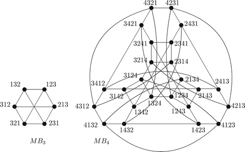
The graphs of $M{B}_3$ and $M{B}_4$ are given in Figure 1.

Figure 1. The modified bubble-sort graphs $M{B}_3$ and $M{B}_4$.

Note that $M{B}_n$ is a special Cayley graph. Therefore, $M{B}_n$ has the following properties.

Proposition 2.1

Lakshmivarahan et al., 1993

For any integer $n\ge 3,$ $M{B}_n$ is vertex transitive and bipartite.

Proposition 2.2

Yu et al., 2013

For any two distinct vertices u and v in $M{B}_n,$ $|N\left(u\right)\cap N\left(v\right)|\le 2,$ when $uv\notin E\left(M{B}_n\right);$ $|N\left(u\right)\cap N\left(v\right)|=0,$ when $uv\in E\left(M{B}_n\right)$ for $n\ge 4$.

Proposition 2.3

Yu et al., 2013

Let $M{B}_n^i$ be defined as above. For any $u,v\in V\left(M{B}_n^i\right),$ each of u and v has two distinct outside neighbours, $\{u^{+},u^{-}\}\cap \{v^{+},v^{-}\}=\mathrm{\varnothing }$ for $i\in [1,n]$.

Proposition 2.4

Yu et al., 2013

Let $\left(u_1{u}_2{u}_3{u}_4\right)$ be a 4-cycle in $M{B}_n$. Then $u_2=u_1\left(ij\right),$ $u_3=u_2\left(kl\right),$ $u_4=u_3\left(ij\right),$ $u_1=u_4\left(kl\right)$ for $i,j,k,l\in [1,n]$ and i, j, k, l differ from each other.

Proposition 2.5

Wang & Wang

$\kappa \left(M{B}_n\right)=n$.

Proposition 2.6

Li et al., 2016

$\kappa \left(B_n\right)=n-1$.

Proposition 2.7

Yu et al., 2013

${\kappa }^{\left(2\right)}\left(M{B}_n\right)=4n-8$ for $n\ge 4$.

3. The 2-good-neighbour diagnosability of the modified bubble-sort graph under the PMC model

In this section, we will give the 2-good-neighbour diagnosability of the modified bubble-sort graph $t_2\left(M{B}_n\right)$ under the PMC model.

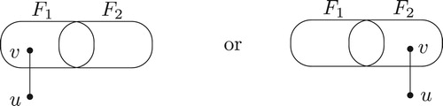
Theorem 3.1

Yuan et al., 2015

A system $G=(V,E),$ let $F_1$ and $F_2$ be the distinct pair of g-good-neighbour faulty subsets of V with $|F_1|\le t$ and $|F_2|\le t$. G is g-good-neighbour t-diagnosable under the PMC model if and only if there is an edge $uv\in E$ with $u\in V\mathrm{\setminus }(F_1\cup F_2)$ and $v\in F_1\mathrm{\Delta }{F}_2$ (Figure 2).

Figure 2. An illustration of a distinguishable pair $(F_1,F_2)$ under the PMC model.

Lemma 3.2

Let D be a subgraph of $M{B}_n$ such that $\delta \left(D\right)=2$. Then $|V\left(D\right)|\ge 4$.

The proof of Lemma 3.2 is trivial.

Lemma 3.3

Let $A=\{u_2=u_1(ij),u_3=u_2(kl),u_4=u_3(ij),u_1=u_4(kl\left)\right\}$ and $M{B}_n$ be defined as above for $i,j,k,l\in [1,n]$ and i, j, k, l differ from each other. Let $F_1=N_{M{B}_n}\left(A\right)$ and $F_2=A\cup N_{M{B}_n}\left(A\right)$. Then $|F_1|=4n-8,$ $|F_2|=4n-4,$ $\delta (M{B}_n-F_1)\ge 2,$ and $\delta (M{B}_n-F_2)\ge 2$ for $n\ge 4$.

Proof.

By Proposition 2.4, $\left(u_1{u}_2{u}_3{u}_4\right)$ is a 4-cycle and A is the vertex set of the 4-cycle. Any two adjacent vertices in A has no common neighbour, $u_1$ has two common neighbours with $u_3$ and $u_2$ has two common neighbours with $u_4$. Then each pair of the vertices in A has no other common neighbour by Proposition 2.2. Combining this with Proposition 2.5, we have that $|N_{M{B}_n}\left(A\right)|=|F_1|=4(n-2)=4n-8$ and $|F_2|=|F_1|+|A|=4n-8+4=4n-4$.

For any vertex $x_1\in V(M{B}_n-F_1)$, it can only connect one of $u_i$ for $i\in [1,4]$. Otherwise, if $x_1$ connects two adjacent vertices in A, then there is an odd cycle in $M{B}_n$, a contradiction to Proposition 2.1. If $x_1$ connects $u_1$ and $u_3$, then $u_1$ and $u_3$ has three common neighbours $u_2$, $u_4$ and $x_1$, a contradiction to Proposition 2.2. By Proposition 2.5, $d\left(x_1\right)=n$. Combining this with $x_1\in V(M{B}_n-F_1)$, we have $d\left(x_1\right)\ge n-1$. Therefore, $\delta (M{B}_n-F_1)\ge 2$ for $n\ge 4$. Let $x_2\in V(M{B}_n-F_2)$. Then $|N_{M{B}_n}\left(x_2\right)\cap F_1|\le 2$ by Proposition 2.2. If $x_2$ has one common neighbour $v\in F_1$ with $u_1$ and one common neighbour $y\in F_1$ with $u_2$, then there is an odd cycle $\left(u_{1}v{x}_{2}y{u}_2\right)$ in $M{B}_n$, a contradiction to Proposition 2.1. If $x_2$ has one common neighbour $v\in F_1$ with $u_1$ and one common neighbour $z\in F_1$ with $u_4$, we get the same contradiction as above. So $x_2$ may have common neighbours with $u_3$. Combining this with Proposition 2.2, we have that $x_2$ may have at most two common neighbours with each of $u_1$ and $u_3$. So $x_2$ may have at most four common neighbours with the vertices of A. By Proposition 2.5, $d\left(x_2\right)=n$. Combining this with $x_2\in V(M{B}_n-F_2)$, we have $d\left(x_2\right)\ge n-4$. Therefore, $\delta (M{B}_n-F_2)\ge 2$ for $n\ge 6$.

Let n = 4 and $A_1=\{u_1=(1),u_2=u_1(12),u_3=u_2(34),u_4=u_3(12\left)\right\}$. Obviously, $\left(u_1{u}_2{u}_3{u}_4\right)$ is a 4-cycle and $A_1$ is the vertex set of the 4-cycle (see Figure 1). Then $|F_1|=|N_{M{B}_4}\left(A_1\right)|=|\left\{u_1\right(23)=1324,u_1(14)=4231;u_2(23)=2314,u_2(14)=4132;u_3(23)=2413,u_3(14)=3142;u_4(23)=1423,u_4(14)=3241\}|=8=4\times 4-8$. $|F_2|=|F_1|+|A|=8+4=12=4\times 4-4$. For any $x\in V(M{B}_4-F_1)$ and $y\in V(M{B}_4-F_2)$, we have $d\left(x\right)\ge 3$ and $d\left(y\right)\ge 3$. Therefore, $\delta (M{B}_4-F_1)>2$ and $\delta \left(M{B}_4-F_2\right)>2$.

Let n = 5. By Proposition 2.4, the 4-cycle in $M{B}_n$ has two types. The first type is none of i, j, k, l is equal to n. Without loss of generality, let $A_2=\{u_1=(1),u_2=u_1(12)=21345,u_3=u_2(34)=21435,u_4=u_3(12)=12435\}$. In this case, We decompose $M{B}_5$ along the last position, denoted by $M{B}_5^i$ for $i\in [1,5]$. Note that $M{B}_5^i\cong B_4$. By the definition of $M{B}_n$, we have that $A_2\subset V\left(M{B}_5^5\right)$, and $|N_{M{B}_5^5}\left(A_2\right)|=|\{13245,23145,24135,14235\}|=4$. By Proposition 2.3, we have that $|N\left(A_2\right)\cap V\left(M{B}_5^4\right)|=|\{u_1^{-}=12354,u_2^{-}=21354\}|=2$, $|N\left(A_2\right)\cap V\left(M{B}_5^3\right)|=|\{u_3^{-}=21453,u_4^{-}=12453\}|=2$, $|N\left(A_2\right)\cap V\left(M{B}_5^2\right)|=|\{u_2^{+}=51342,u_3^{+}=51432\}|=2$, and $|N\left(A_2\right)\cap V\left(M{B}_5^1\right)|=|\{u_1^{+}=52341,u_4^{+}=52431\}|=2$. Therefore, $|F_1|=|N_{M{B}_5}\left(A_2\right)|=4+2+2+2+2=12=4\times 5-8$ and $|F_2|=|F_1|+|A|=12+4=16=4\times 5-4$. Note that $N\left(A_2\right)\cap V\left(M{B}_5^j\right)$ is a $K_2$ and $M{B}_5^j\cong B_4$ for $j\in [1,4]$. Each $K_2$ in $M{B}_5^j$ has no other common neighbour by Proposition 2.2. Combining this with Proposition 2.6, we have that $M{B}_5^j-N_{M{B}_5^j}\left(A_2\right)$ is connected and $\delta (M{B}_5^j-N_{M{B}_5^j}(A_2\left)\right)\ge 2$ for $j\in [1,4]$. Note that A is a 4-cycle, $\delta \left(A\right)=2$. Meanwhile, the vertices in $N_{M{B}_5^5}\left(A_2\right)=\{13245,23145,24135,14235\}$ are different and disconnected. Combining $M{B}_5^5\cong B_4$ with Proposition 2.6, we have $\delta (M{B}_5^5-N_{M{B}_5^j}(A_2\left)\right)\ge 3-1=2$. Therefore, $\delta (M{B}_5-F_1)\ge 2$. Since $|A\cap V\left(M{B}_5^j\right)|=0$, we have $\delta (M{B}_5^j-F_2)\ge 2$ by the above for $j\in [1,4]$. Let $x_3\in V\left(M{B}_5^5\right)$. By the definition of $M{B}_5$, we have that the neighbours of $N_{M{B}_5^5}\left(A_2\right)$ are $\{13425,31245;32145,23415;42135,24315;41235,14325\}$. Obviously, the vertices in $N_{M{B}_5^5}\left(A_2\right)\subset F_1$ have no common neighbour. So $\delta \left(x\right)\ge 3-1=2$. Therefore, $\delta (M{B}_5-F_2)\ge 2$. The proof is complete.

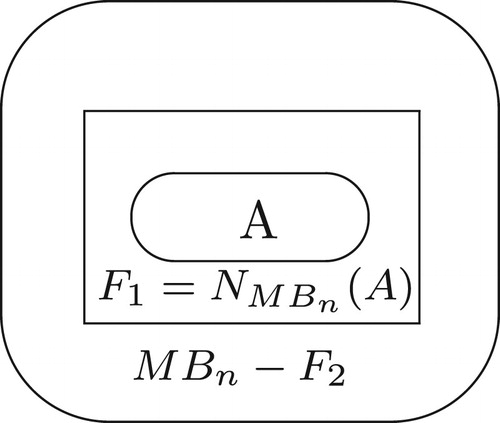
Lemma 3.4

For $n\ge 4,$ $t_2\left(M{B}_n\right)\le 4n-5$.

Proof.

Let A be defined as above and let $F_1=N_{M{B}_n}\left(A\right)$, $F_2=A\cup N_{M{B}_n}\left(A\right)$ (see Figure 3). By Lemma 3.3, we have that $|F_1|=4n-8$, $|F_2|=4n-4$, $\delta (M{B}_n-F_1)\ge 2$ and $\delta (M{B}_n-F_2)\ge 2$ for $n\ge 4$. Therefore, $F_1$ and $F_2$ are both 2-good-neighbour faulty sets of $M{B}_n$. Note that $A=F_1\mathrm{\Delta }{F}_2$ and $N_{M{B}_n}\left(A\right)=F_1\subset F_2$. There is no edge of $M{B}_n$ between $V\left(M{B}_n\right)\mathrm{\setminus }(F_1\cup F_2)$ and $F_1\mathrm{\Delta }{F}_2$. By Theorem 3.1, we have that $M{B}_n$ is not 2-good-neighbour $(4n-4)$-diagnosable under the PMC model. Hence, by the definition of 2-good-neighbour diagnosability, we conclude that the 2-good-neighbour diagnosability of $M{B}_n$ is less than 4n−4. Then $t_2\left(M{B}_n\right)\le 4n-5$.

Figure 3. An illustration about the proofs of Lemmas 3.3, 3.4 and 4.2.

Lemma 3.5

For $n\ge 4,$ $t_2\left(M{B}_n\right)\ge 4n-5$.

Proof.

By the definition of 2-good-neighbour diagnosability, it is sufficient to show that $M{B}_n$ is 2-good-neighbour $(4n-5)$-diagnosable. By Theorem 3.1, to prove that $M{B}_n$ is 2-good-neighbour $(4n-5)$-diagnosable, it is equivalent to prove that there is an edge $uv\in E\left(M{B}_n\right)$ with $u\in V\left(M{B}_n\right)\mathrm{\setminus }(F_1\cup F_2)$ and $v\in F_1\mathrm{\Delta }{F}_2$, $F_1$ and $F_2$ are distinct 2-good-neighbour faulty subsets of $V\left(M{B}_n\right)$ with $|F_1|\le 4n-5$ and $|F_2|\le 4n-5$.

We prove this statement by contradiction. Suppose that there are two distinct 2-good-neighbour faulty subsets $F_1$ and $F_2$ of $V\left(M{B}_n\right)$ with $|F_1|\le 4n-5$ and $|F_2|\le 4n-5$. But the vertex set pair $(F_1,F_2)$ does not satisfy the conditions of Theorem 3.1, i.e. there is no edge between $V\left(M{B}_n\right)\mathrm{\setminus }(F_1\cup F_2)$ and $F_1\mathrm{\Delta }{F}_2$. Without loss of generality, we assume that $F_2\mathrm{\setminus }{F}_1\ne \mathrm{\varnothing }$. Now, we will show the contradiction.

Case 1. $V\left(M{B}_n\right)=F_1\cup F_2$.

By the definition of $M{B}_n$, $|V\left(M{B}_n\right)|=n!=|F_1\cup F_2|$. It is obvious that $n!>8n-10$ for $n\ge 4$. But $n!=|V\left(M{B}_n\right)|=|F_1\cup F_2|=|F_1|+|F_2|-|F_1\cap F_2|\le |F_1|+|F_2|\le 2(4n-5)=8n-10$, a contradiction. Therefore, $V\left(M{B}_n\right)\ne F_1\cup F_2$.

Case 2. $V\left(M{B}_n\right)\ne F_1\cup F_2$.

Note that there is no edge between $V\left(M{B}_n\right)\mathrm{\setminus }(F_1\cup F_2)$ and $F_1\mathrm{\Delta }{F}_2$, and $F_1$ is a 2-good-neighbour faulty set. Let $M{B}_n-F_1-F_2$ and $M{B}_n\left[F_2\mathrm{\setminus }{F}_1\right]$ be two parts of $M{B}_n-F_1$. Then $\delta (M{B}_n-F_1-F_2)\ge 2$ and $\delta \left(M{B}_n\right[F_2\mathrm{\setminus }{F}_1\left]\right)\ge 2$. Similarly, we have $\delta \left(M{B}_n\right[F_1\mathrm{\setminus }{F}_2\left]\right)\ge 2$ when $F_1\mathrm{\setminus }{F}_2\ne \mathrm{\varnothing }$. Therefore, $F_1\cap F_2$ is a 2-good-neighbour faulty set. When $F_1\mathrm{\setminus }{F}_2=\mathrm{\varnothing }$, $F_1\cap F_2=F_1$ is also a 2-good-neighbour faulty set. Since there is no edge between $V\left(M{B}_n\right)\mathrm{\setminus }(F_1\cup F_2)$ and $F_1\mathrm{\Delta }{F}_2$, $F_1\cap F_2$ is a 2-good-neighbour cut. By Proposition 2.7, $|F_1\cap F_2|\ge 4n-8$ for $n\ge 4$. Meanwhile, by Lemma 3.2, we have $|F_2\setminus F_1|\ge 4$. Consequently, $|F_2|=|F_2\setminus F_1|+|F_1\cap F_2|\ge 4+4n-8=4n-4$, which is a contradiction to $|F_2|\le 4n-5$. In conclusion, $M{B}_n$ is 2-good-neighbour $(4n-5)$-diagnosable. By the definition of $t_2\left(M{B}_n\right)$, we have $t_2\left(M{B}_n\right)\ge 4n-5$.

Combining Lemma 3.4 with Lemma 3.5, we have the following theorem.

Theorem 3.6

The 2-good-neighbour diagnosability of $M{B}_n$ under the PMC model is 4n−5 for $n\ge 4$.

4. The 2-good-neighbour diagnosability of the modified bubble-sort graph under the $M{M}^{\ast }$ model

In this section, we will show the 2-good-neighbour diagnosability of the modified bubble-sort graph $t_2\left(M{B}_n\right)$ under the $M{M}^{\ast }$ model.

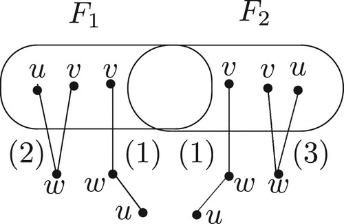
Theorem 4.1

Dahbura & Masson, 1984; Yuan et al., 2015: A system $G=(V,E)$ is g-good-neighbour t-diagnosable under the $M{M}^{\ast }$ model if and only if for each distinct pair g-good-neighbour faulty subsets $F_1$ and $F_2$ of V with $|F_1|\le t$ and $|F_1|\le t$ satisfies one of the following conditions.

1. There are two vertices $u,w\in V\mathrm{\setminus }(F_1\cup F_2)$ and there is a vertex $v\in F_1\mathrm{\Delta }{F}_2$ such that $uw\in E$ and $vw\in E$.

2. There are two vertices $u,v\in F_1\mathrm{\setminus }{F}_2$ and there is a vertex $w\in V\mathrm{\setminus }(F_1\cup F_2)$ such that $uw\in E$ and $vw\in E$.

3. There are two vertices $u,v\in F_2\mathrm{\setminus }{F}_1$ and there is a vertex $w\in V\mathrm{\setminus }(F_1\cup F_2)$ such that $uw\in E$ and $vw\in E$ (See Figure 4).

Figure 4. An illustration of a distinguishable pair $(F_1,F_2)$ under the $M{M}^{\ast }$ model.

Lemma 4.2

For $n\ge 4,$ $t_2\left(M{B}_n\right)\le 4n-5$.

Proof.

Let A, $F_1$ and $F_2$ be defined in Lemma 3.4 (Figure 3). By Lemma 3.4, $|F_1|=4n-8$, $|F_2|=4n-4$, $\delta (M{B}_n-F_1)\ge 2$, $\delta (M{B}_n-F_2)\ge 2$ for $n\ge 4$. So both $F_1$ and $F_2$ are 2-good-neighbour faulty sets. By the definition of $F_1$ and $F_2$, $F_1\mathrm{\Delta }{F}_2=A$ and there is no edge between A and $V\left(M{B}_n\right)\mathrm{\setminus }(F_1\cup F_2)$. Therefore, there is no vertex $v\in F_1\mathrm{\Delta }{F}_2$ and $u,w\in V\left(M{B}_n\right)\mathrm{\setminus }(F_1\cup F_2)$ such that $uw\in E$ and $vw\in E$, the condition (1) of Theorem 4.1 is not satisfied. Meanwhile, $F_1\mathrm{\setminus }{F}_2=\mathrm{\varnothing }$, the condition (2) of Theorem 4.1 is not satisfied. Since $F_2\mathrm{\setminus }{F}_1=A$, there is no edge between A and $V\left(M{B}_n\right)\mathrm{\setminus }(F_1\cup F_2)$, the condition (3) of Theorem 4.1 is not satisfied. Hence, $M{B}_n$ is not 2-good-neighbour $(4n-4)$-diagnosable, i.e. $t_2\left(M{B}_n\right)\le 4n-5$ for $n\ge 4$.

Lemma 4.3

For $n\ge 4,$ $t_2\left(M{B}_n\right)\ge 4n-5$.

Proof.

By the definition of 2-good-neighbour diagnosability, it is sufficient to show that $M{B}_n$ is 2-good-neighbour $(4n-5)$-diagnosable. This statement is proved by contradiction. We suppose that there are two distinct 2-good-neighbour faulty subsets $F_1$ and $F_2$ of $V\left(M{B}_n\right)$ with $|F_1|\le 4n-5$ and $|F_2|\le 4n-5$. But the vertex pair $(F_1,F_2)$ does not satisfy any condition of Theorem 4.1. Without loss of generality, we assume that $F_2\mathrm{\setminus }{F}_1\ne \mathrm{\varnothing }$. Similar to the discussion on $V\left(M{B}_n\right)=F_1\cup F_2$ in Lemma 3.5, we can deduce $V\left(M{B}_n\right)\ne F_1\cup F_2$.

Claim 1

$M{B}_n-F_1-F_2$ has no isolated vertex.

Suppose, on the contrary, that $M{B}_n-F_1-F_2$ has at least one isolated vertex w. Since $F_1$ is a 2-good-neighbour faulty set, there are two vertices $u,v\in F_2\setminus F_1$ such that u, v are connected to w. Since the vertex set pair $(F_1,F_2)$ does not satisfy any condition of Theorem 4.1, this is a contradiction. Therefore, $M{B}_n-F_1-F_2$ has no isolated vertex. The proof of Claim 1 is complete.

Let $u\in V\left(M{B}_n\right)\mathrm{\setminus }(F_1\cup F_2)$. By Claim 1, u has at least one neighbour w in $M{B}_n-F_1-F_2$. Since the vertex set pair $(F_1,F_2)$ does not satisfy any condition of Theorem 4.1, for any pair of adjacent vertices $u,w\in V\left(M{B}_n\right)\mathrm{\setminus }(F_1\cup F_2)$, there is no vertex $v\in F_1\mathrm{\Delta }{F}_2$ such that $uw\in E\left(M{B}_n\right)$ and $wv\in E\left(M{B}_n\right)$. Therefore, u has no neighbour in $F_1\mathrm{\Delta }{F}_2$. By the arbitrariness of u, there is no edge between $V\left(M{B}_n\right)\mathrm{\setminus }(F_1\cup F_2)$ and $F_1\mathrm{\Delta }{F}_2$. Since $F_2\mathrm{\setminus }{F}_1\ne \mathrm{\varnothing }$ and $F_1$ is a 2-good-neighbour faulty set, we have $\delta \left(M{B}_n\right[F_2\mathrm{\setminus }{F}_1\left]\right)\ge 2$. Similarly, $\delta \left(M{B}_n\right[F_1\mathrm{\setminus }{F}_2\left]\right)\ge 2$ when $F_2\mathrm{\setminus }{F}_1\ne \mathrm{\varnothing }$. By Lemma 3.2, $|F_2\mathrm{\setminus }{F}_1|\ge 4$. Since $F_1$ and $F_2$ are 2-good-neighbour faulty sets of $M{B}_n$, and there is no edge between $V\left(M{B}_n\right)\mathrm{\setminus }(F_1\cup F_2)$ and $F_1\mathrm{\Delta }{F}_2$, we have that $(F_1\cap F_2)$ is a 2-good-neighbour cut of $M{B}_n$. By Proposition 2.7, $|F_1\cap F_2|\ge 4n-8$. Therefore, $|F_2|=|F_1\cap F_2|+|F_2\mathrm{\setminus }{F}_1|\ge 4n-8+4=4n-4$, which contradicts $|F_2|\le 4n-5$. Therefore, $M{B}_n$ is 2-good-neighbour $(4n-5)$-diagnosable. Then $t_2\left(M{B}_n\right)\ge 4n-5$ for $n\ge 4$.

Combining Lemma 4.2 with Lemma 4.3, we have the following theorem.

Theorem 4.4

The 2-good-neighbour diagnosability of $M{B}_n$ under the $M{M}^{\ast }$ model is 4n−5 for $n\ge 4$.

5. Conclusions

The modified bubble-sort graph is an important interconnection network topology and it has many good properties. In this paper, we proved that the 2-good-neighbour diagnosability of $M{B}_n$ under the PMC model and $M{M}^{\ast }$ model. The conclusion is that $M{B}_n$ is $(4n-5)$-diagnosable under the PMC model and $M{M}^{\ast }$ model for $n\ge 4$. This work will help engineers to do more further researches based on application environment. Unfortunately, we only discussed the theoretical part, and did not do the relevant applied research. We will do further research in the future.

Disclosure statement

No potential conflict of interest was reported by the author(s).

Additional information

Funding

This work is supported by the National Science Foundation of China (61772010) and the Graduate Quality Curriculum Construction Project of Henan Normal University (5101019500604).

References

- Akers, S. B., & Krishanmurthy, B. (1989). A group-theoretic model symmetric interconnction networks. IEEE Transactions on Computers, 38(4), 555–566. doi: https://doi.org/10.1109/12.21148
- Bondy, J. A., & Murty, U. S. R. (2007). Graph theory. Springer.
- Cheng, E., & Lipták, L. (2007). Fault resiliency of Cayley graphs generated by transpositions. International Journal of Foundations of Computer Science, 18(5), 1005–1022. doi: https://doi.org/10.1142/S0129054107005108
- Dahbura, A. T., & Masson, G. M. (1984). An O(n2.5) fault identification algorithm for diagnosable systems. IEEE Transactions on Computers, 33(6), 486–492. doi: https://doi.org/10.1109/TC.1984.1676472
- Fan, J. (2002). Diagnosability of crossed cubes under the comparison diagnosis model. IEEE Transactions on Parallel and Distributed Systems, 13(10), 1099–1104. doi: https://doi.org/10.1109/TPDS.2002.1041887
- Lai, P.-L., Tan, J. J. M., Chang, C.-P., & Hsu, L.-H. (2005). Conditional diagnosability measures for large multiprocessor systems. IEEE Transactions on Computers, 54(2), 165–175. doi: https://doi.org/10.1109/TC.2005.19
- Lakshmivarahan, S., Jwo, J., & Dhall, S. K. (1993). Symmetry in interconnection networks based on Cayley graphs of permutation groups: A survey. Parallel Computing, 19(4), 361–407. doi: https://doi.org/10.1016/0167-8191(93)90054-O
- Li, S., Tu, J., & Yu, C. (2016). The generalized 3-connectivity of star graphs and bubble-sort graphs. Applied Mathematics and Computation, 274, 41–46. doi: https://doi.org/10.1016/j.amc.2015.11.016
- Maeng, J., & Malek, M. (1981). A comparison connection assingment for self-diagnosis of multiprocessor systems. In Conte, T. M. (Ed.), Proceedings of the 11th international symposium on fault tolerant computing (pp. 173–175). IEEE Computer Society Press.
- Peng, S.-L., Lin, C.-K., Tan, J. J. M., & Hsu, L.-H. (2012). The g-good-neighbor conditional diagnosability of hypercubes under PMC model. Applied Mathematics and Computation, 218(21), 10406–10412. doi: https://doi.org/10.1016/j.amc.2012.03.092
- Preparata, F. P., Metze, G., & Chien, R. T. (1967). On the connection assignment problem of diagnosable systems. IEEE Transactions on Electronic Computers, EC-16(12), 848–854. doi: https://doi.org/10.1109/PGEC.1967.264748
- Wang, S., & Han, W. (2016). The g-good-neighbor diagnosability of the n-dimensional hypercube under the MM∗ model. Information Processing Letters, 116(9), 574–577. doi: https://doi.org/10.1016/j.ipl.2016.04.005
- Wang, M., Lin, Y., & Wang, S. (2016). The 2-good-neighbors diagnosability of cayley graphs generated by transposition trees under the PMC model and MM∗ model. Theoretical Computer Science, 628, 92–100. doi: https://doi.org/10.1016/j.tcs.2016.03.019
- Wang, S., Wang, Z., & Wang, M. (2017). The 2-good-neighbor connectivity and 2-good-neighbor diagnosability of bubble-sort star graph networks. Discrete Applied Mathematics, 217, 691–706. doi: https://doi.org/10.1016/j.dam.2016.09.047
- Wang, Y., & Wang, S. The 3-good-neighbor connectivity of modified bubble-sort graphs [Unpublished].
- Wang, Y., & Wang, S. The 3-good-neighbor diagnosability of modified bubble-sort graphs under the PMC and MM∗ model [Unpublished].
- Yu, X., & Huang, X. (2012). Restricted vertex connectivity of modified bubble-sort graphs. Journal of Xinjiang University, 29(1), 78–81.
- Yu, X., Huang, X., & Zhang, Z. (2013). A kind of conditional connectivity of Cayley graphs generated by unicyclic graphs. Information Sciences, 243, 86–94. doi: https://doi.org/10.1016/j.ins.2013.04.011
- Yuan, J., Liu, A., Ma, X., Liu, X., Qin, X., & Zhang, J. (2015). The g-good-neighbor conditional diagnosability of k-ary n cubes under the PMC model and MM∗ model. IEEE Transactions on Parallel and Distributed Systems, 26(4), 1165–1177. doi: https://doi.org/10.1109/TPDS.2014.2318305