An improved algorithm for incremental extreme learning machine

Abstract

Incremental extreme learning machine (I-ELM) randomly obtains the input weights and the hidden layer neuron bias during the training process. Some hidden nodes in the ELM play a minor role in the network outputs which may eventually increase the network complexity and even reduce the stability of the network. In order to avoid this issue, this paper proposed an enhanced method for the I-ELM which is referred to as the improved incremental extreme learning machine (II-ELM). At each learning step of original I-ELM, an additional offset k will be added to the hidden layer output matrix before computing the output weights for the new hidden node and analysed the existence of the offset k. Compared with several improved algorithms of ELM, the advantages of the II-ELM in the training time, the forecasting accuracy, and the stability are verified on several benchmark datasets in the UCI database.

KEYWORDS:

• Extreme learning machine
• incremental algorithm
• random hidden nodes
• single-hidden layer feedforward neural networks

1. Introduction

The original extreme learning machine (ELM) (Huang, 2015; Huang et al., 2004) is a supervised learning algorithm based on the single-hidden layer feedforward neural networks (SLFNs) (Huang et al., 2015; Huang, Zhu, et al., 2006). Compared with other several neural networks, such as the back propagation (BP) networks (Wang et al., 2015), the support vector machine (SVM)(Yang et al., 2019), the ELM only needs to set up the number of the hidden nodes, and does not need to adjust the input weights repeatedly, which has tremendous profits including the less human-interface, the faster learning speed, the promising generalization capability, and, etc. (Cao et al., 2020; Cui et al., 2018; Song et al., 2018). As the same, there are also advantages of ELM in the classification problems and have been validated in the literature (Inaba et al., 2018; Zhao et al., 2011).

However, there are some shortcomings of the ELM. For example, the input weights and the bias of hidden nodes of the ELM network are randomly obtained, which results in poor network stability to a certain extent. When there are outliers or disturbances in the training data, the ill-conditioned problems will exist in the output matrix of the hidden layer, which leads to the poor network robustness, the reduced generalization performance, and the reduced forecasting accuracy.

At present, ELM has been widely studied. The ELM can be divided into the fixed ELM and the incremental extreme learning machine (I-ELM) (Huang, Chen, et al., 2006). The training process of the fixed ELM is one-shot computation with the fast learning speed (Song et al., 2015). Nevertheless, how to choose the best number of hidden layer neurons and the optimal weights and bias in the fixed ELM is a difficult problem. The literature (Cheng et al., 2019) proposes an improved training method for ELM with Genetic Algorithms to get the optimal weights and bias after selection, crossover and mutation. An ELM model based on the differential evolution improved whale optimization algorithm is proposed in the literature (Zhou et al., 2020), and is applied in the colour difference classification. The literature (Zhou, Wang, et al., 2019) proposes a hybrid grey wolf optimization algorithm based on fuzzy weights and a differential evolution algorithm to overcome the problems of ELM, which randomly selects hidden layer weights and biases. Furthermore, the ELM is suitable for the classification (Sun et al., 2019), the image processing (Zhou, Gao, et al., 2019; Zhou, Chen, Song, Zhu & Liu), and the online fault diagnose (Zhou, Bo, et al., 2019), etc.

Compared with the ELM, I-ELM has the characteristics that the output error gradually decreases and is close to zero as the number of hidden neurons increases (Huang, Chen, et al., 2006). It is suitable for regression and classification problems in online continuous learning (Xu & Wang, 2016; Zhang et al., 2019). However, the training speed of the I-ELM is not as fast as that of the ELM because the number of the computation times of output weights is equal to the number of hidden layer nodes. The input weights and the bias of hidden nodes of the I-ELM are also obtained randomly, which will cause the following two problems. First, some of the hidden neurons may play minor roles on the output of the network as their output weights are too small, which makes the learning speed of the network further slowdown. Secondly, these invalid hidden layer neurons will increase the complexity of the network, and slow down the error reduction in training process. To deal with these problems, there have been put forward some improved methods. In (Wu et al., 2017) length-changeable incremental extreme learning machine (LCI-ELM) is proposed and improved the generalization performance by adding the number of hidden nodes, but it is difficult to determine the number of neurons increased in the hidden layer optimally. The literature (Zhou et al., 2018) proposes the regularization incremental extreme learning machine with random reduced kernel (RKRIELM) algorithm which combines the kernel function and incremental I-ELM to avoid randomness. In (Li et al., 2018) an effective hybrid approach based on variable-length incremental ELM and particle swarm optimization algorithm (PSO-VIELM) is proposed to determine the proper hidden nodes and corresponding number in input weights and hidden bias, but the learning speed has decreased.

This paper proposes an improved I-ELM algorithm which is referred to as the improved incremental extreme learning machine (II-ELM) by adding an offset k to the hidden-layer output to obtain the optimal weights. The essential difference between the offset k in the II-ELM and the bias of the hidden nodes is that the bias is randomly determined before computing the output weights of the hidden-layer, whereas the offset k in the II-ELM is obtained after the output weights. The existence of the offset k is discussed, and the validity of the II-ELM is also demonstrated by comparing it with the I-ELM, convex incremental extreme learning machine (CI-ELM) (Huang & Chen, 2007), enhanced method for incremental extreme learning machine (EI-ELM) (Huang & Chen, 2008), bidirectional extreme learning machine (B-ELM) (Yang et al., 2012), self-adaptive differential evolution and the extreme learning machine (SaDE-ELM) (Cao et al., 2012), enhanced bidirectional extreme learning machine (EB-ELM) (Cao et al., 2019), and genetic algorithm extreme learning machine (GA-ELM) (Cheng et al., 2019) on the regression and classification problems from UCI database.

The rest of the paper will be organized as follows. Section 2 briefly reviews the basic principles of I-ELM. Section 3 proposes the improved algorithm for the I-ELM. Comparisons of the simulation and evaluation of the results are presented in Section 4. The conclusion is arranged in the section 5.

2. Brief review of I-ELM

The structure of the I-ELM network is shown in Figure 1. It is composed of m inputs, l hidden nodes, and n outputs. ω_i is the 1×m input weight matrix of the current hidden layer neuron, whose entries are random numbers uniformly distributed between [−1, 1].

Figure 1. The structure of I-ELM network.

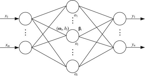
b_iis the bias of the i-th hidden node, and its value is a random number uniformly distributed between [−1, 1] when the activation function for the hidden layer neuron is the additive type corresponding to (1). β is the l×n output weight matrix.

The activation function for additive hidden nodes is given below: (1) $\begin{array}{r}g\left(\mathbf{x}\right)=\frac{1}{1+\exp (-\mathbf{x})}\end{array}$(1) where x is the input matrix.

Given a training set{(X, Y)}, where X is a m×N matrix that represents the input of N data sets and Y is a n×N matrix that represents the output of N data sets. The training steps of the I-ELM algorithm will be summarized as follows:

Step 1: Initialization. Let l=0, the maximum number of the hidden nodes is set to be L, and the expected training accuracy is set to be ϵ. The initial value of the residuals E (the error between the actual output and the target output of the network) is set to be the output Y.

Step 2: Training steps. While l < L and ‖E‖ > ϵ

1. The number of the hidden nodes l increase by 1: l = l+1.

2. The input weights ω_l and bias b_l of the newly increased hidden layer neuron o_l is obtained randomly.

3. Calculate the output of the activation function g(x’) for the node o_l. (It is needed to extend b_l into a 1×N vector b_l.) (2) $\begin{array}{r}{\mathbf{x}}^{\mathrm{\prime }}={\mathit{\omega }}_l\mathbf{X}+{\mathbf{b}}_l\end{array}$(2)

4. Calculate the output vector $\overline{\mathbf{H}}$ of hidden layer neurons: (3) $\begin{array}{r}\overline{\mathbf{H}}=g\left({\mathbf{x}}^{\mathrm{\prime }}\right)\end{array}$(3)

5. Calculate the output weight for o_l: (4) $\begin{array}{r}\overline{\text{β}}=\frac{\mathbf{E}\bullet {\overline{\mathbf{H}}}^{\text{T}}}{\overline{\mathbf{H}}\bullet {\overline{\mathbf{H}}}^{\text{T}}}\end{array}$(4)

6. Calculate the residuals error after increasing the new hidden node: (5) $\begin{array}{r}{\mathbf{E}}^{\mathrm{\prime }}=\mathbf{E}-\overline{\text{β}}\overline{\mathbf{H}}\end{array}$(5)

The output weight obtained from (4) is capable of decreasing the error of the network at the fastest speed. Above steps should be repeated until the residuals is smaller than the expected error ϵ. Otherwise, when l > L and the error is still larger than the expected error ϵ, the training process should be restarted. In most of the cases, it is caused by the random determination of the input weight ω_l and the bias b_l, so one should restart the training process.

Finally, according to the given testing set {(X’, Y’)}, one can test whether the trained network meets the requirements or not.

3. Proposed improved algorithm for the I-ELM(II-ELM)

To address the problem that the residuals of the I-ELM network declines slowly in its training process, an improved algorithm is proposed in this section. First, the hidden-layer output matrix H is adjusted by adding an additional offset k to the output weights. Then the output weight β’ is calculated to generate the updated output matrix H’. It should be noted that for some cases, the network is optimal with k equal to 0, which means that the hidden nodes do not need to add the offset k. The computation process of offset k is as follows.

It is assumed that E = [e₁,e₂, … ,e_N], H = [h₁,h₂, … ,h_N], the value of the offset is k, and H'=[(h₁+k),(h₂+k), … , (h_N+k)]. The following part shows how to obtain the optimal value of k.

1. Calculate the residuals error Z’ between E and H':

According to (4), the output weight β’ at this point is (6) $\begin{array}{r}{\text{β}}^{\mathrm{\prime }}=\frac{\mathbf{E}\bullet {{\mathbf{H}}^{\mathrm{\prime }}}^{\text{T}}}{{\mathbf{H}}^{\mathrm{\prime }}\bullet {{\mathbf{H}}^{\mathrm{\prime }}}^{\text{T}}}=\frac{\sum _{i=1}^N{e}_i\left(h_i+k\right)}{\sum _{i=1}^N{\left(h_i+k\right)}^2}\end{array}$(6) The root mean square error, denoted as Z’, is calculated as follows: (7) $\begin{array}{r}{Z}^{\mathrm{\prime }}=\sqrt{\frac{1}{N}\sum _{i=1}^N{\left(e_i-{\text{β}}^{\mathrm{\prime }}(h_i+k)\right)}^2}\end{array}$(7) Substitute the value of β’ obtained by (6) into (7): (8) $\begin{array}{r}{Z}^{\mathrm{\prime }}=\sqrt{\frac{1}{N}\left(\sum _{i=1}^N{e}_i^2-\frac{{\left(\sum _{i=1}^N{e}_i\left(h_i+k\right)\right)}^2}{\sum _{i=1}^N{\left(h_i+k\right)}^2}\right)}\end{array}$(8) From (7), it is obvious that the value of Z’ is always greater than or equal to zero regardless of the value of k. It means that the value of k can be in the range of (-∞, +∞).

(2)	Calculate the value of k that minimizes Z’

To minimize Z’, the derivative of (9) can be taken: (9) $\begin{array}{r}y\left(k\right)=\sum _{i=1}^N{e}_i^2-\frac{{\left(\sum _{i=1}^N{e}_i\left(h_i+k\right)\right)}^2}{\sum _{i=1}^N{\left(h_i+k\right)}^2}\end{array}$(9) Defining the following variables: $a_1={\left(\sum _{i=1}^N{e}_i\right)}^2$, $a_2=2\left(\sum _{i=1}^N{e}_i\right)\left(\sum _{i=1}^N{e}_i{h}_i\right)$, $a_3={\left(\sum _{i=1}^N{e}_i{h}_i\right)}^2$, b₁= N, $b_{\text{2}}\text{ = 2}\sum _{i\text{ = 1}}^N{h}_{\text{i}}$, and $b_3=\sum _{i=1}^N{h}_i^2$, then the derivative of (9) can be written as: (10) $\begin{array}{r}{y}^{\mathrm{\prime }}\left(k\right)=-\frac{\begin{array}{c}\left(a_1{b}_2-a_2{b}_1\right)k^2+2\left(a_1{b}_3-a_3{b}_1\right)k\\ +\left(a_2{b}_3-a_3{b}_2\right)\end{array}}{{\left(b_1{k}^2+b_{2}k+b_3\right)}^2}\end{array}$(10)

To calculate the extreme of y(k) in (9), denote c₁ = a₁b₂−a₂b₁, c₂ = 2(a₁b₃−a₃b₂), c₃ = a₂b₃−a₃b₂, and let y′(k) = 0.

Assuming that the derivative y′(k) = 0 has no solution, i.e. b₁k² + b₂k + b₃=0, and $\sum _{i=1}^N{(h_i+k)}^2=b_1{k}^2+b_{2}k+b_3$, the entries in H must be all equal. When the entries in H are all equal, one has $a_1/b_1=a_2/b_2=a_3/b_3=(\sum _{i=1}^N{e}_i{)}^2/N$. However, from (9), $y\left(k\right)=\sum _{i=1}^N{e}_i^2-(\sum _{i=1}^N{e}_i{)}^2/N$ is a constant value and its derivative y′(k) = 0. Therefore, the assumption is invalid, namely, there is no point where the derivative y′(k) = 0 has no solution.

The extreme point k obtained by (10) is also the extreme point of Z’ in (7) and (8). The minimum k value of Z’ is in the extreme point, the derivative-free solution point, and the boundary point (k=+∞ or k=-∞), respectively.

However, when k=+∞ or k=-∞, the output weight β’ is zero according to (6), which is not suitable. Furthermore, if the derivative y′(k) has no solution, the value of k, which is capable of minimizing Z’, is at the extreme points. This value of k should be taken and the corresponding output weight β’ should be calculated. When the value of k minimizes the Z’ and k is on the boundary points, the hidden layer node is invalid. When Z’ is a constant value (the entries in the hidden layer output matrix H’ are all equal, which is highly unlikely), the reduction of the network error is the same regardless of the value of k. therefore, k can be set at 0 and the corresponding output weight β’ can be calculated accordingly.

Several types of extreme points of y(k) are discussed as follows:

1. c₁≠0.

The equation y′(k) = 0 can be considered as solving a single variable quadratic equation. One should determine whether its solution exists or not.

Let $a_2^2=4a_1{a}_3$, and its discriminant is evaluated: (11) $\begin{array}{r}\Delta =c_2^2-4c_1{c}_3=[2\left(a_1{b}_3+a_3{b}_1\right)-a_2^2{b}_2^2{]}^2\ge 0\end{array}$(11) Because Δ≥0, there are two possible values for the extreme point k, denoted as k₁ or k₂: (12) $\begin{array}{rl}{k}_1& =\frac{-c_2+\sqrt{c_2^2-4c_1{c}_3}}{2c_1}\end{array}$(12) (13) $\begin{array}{rl}{k}_2& =\frac{-c_2-\sqrt{c_2^2-4c_1{c}_3}}{2c_1}\end{array}$(13) When Δ>0, the two extreme points are not the same: one is the minimum point, and the other is the maximum point.

In this case, y′(k) =−(k−k₁)(k−k₂)/(b₁k² + b₂k + b₃)². The error Z’ rises or decreases monotonically when y′(k) > 0 or y′(k) < 0, respectively. So, it can be concluded that when k ranges from the negative infinite to the positive infinite, the error Z’ will first increase gradually from the error e (the error before adding the current new hidden node) to the maximum, then decrease gradually to a minimum value, and finally increase gradually to the error e (or is just the reverse of the above process). Therefore, the minimum point can minimize the error Z’. By substituting these two extreme points into (8), the global minimum for Z’ in (8) can be calculated, and then the corresponding output weight β’ can be obtained by (6).

When Δ = 0, the two extreme points merge to one, then (14) $\begin{array}{r}2(a_1{b}_3+a_3{b}_1)-a_2{b}_2=0\end{array}$(14) Because $a_2^2=4a_1{a}_3$, as long as one of a₁, a₂, and a₃ is zero, the other two are also zero (b₁=N≠0, b₃>0, the probability that all entries in H are equal is almost zero). If a₁, a₂, and a₃ are all zero, then, c₁=0, which violates the previous assumption. Thus, a₁, a₂, and a₃ are all nonzero. Therefore, (14) can be written as: (15) $\begin{array}{r}\frac{b_1}{a_1}+\frac{b_3}{a_3}=2\frac{b_2}{a_2}\end{array}$(15)

Given the fact that a₁, a₃, b₁, and b₃ are greater than zero, (15) can be written as (16) $\begin{array}{r}{\left(\frac{\sqrt{b_1}}{\sqrt{a_1}}-\frac{\sqrt{b_3}}{\sqrt{a_3}}\right)}^2+2\frac{\sqrt{b_1}}{\sqrt{a_1}}\frac{\sqrt{b_3}}{\sqrt{a_3}}-2\frac{b_2}{a_2}=0\end{array}$(16) Since $a_2^2=4a_1{a}_3$, let $4b_1{b}_3>b_2^2$, and divide both sides of $4b_1{b}_3>b_2^2$ by $a_2^2$: (17) $\begin{array}{r}\frac{\sqrt{b_1}}{\sqrt{a_1}}\frac{\sqrt{b_3}}{\sqrt{a_3}}\ge \frac{b_2}{a_2}\end{array}$(17)

According to (16) and (17), one can have (18) $\begin{array}{r}\frac{b_1}{a_1}=\frac{b_3}{a_3}\end{array}$(18) Substituting (18) into (15), one has (19) $\begin{array}{r}\frac{b_1}{a_1}=\frac{b_2}{a_2}=\frac{b_3}{a_3}\end{array}$(19)

Then c₁ will be equal to zero, which violates the previous assumption. It can be concluded that c₁=0 when Δ=0. Therefore, it can be concluded that Δ≠0 when c₁≠0.

(2)	If c1=0 and c2≠0, the value of extreme point k is: (20) $\begin{array}{r}k=-\frac{c_3}{c_2}\end{array}$(20)

Because c₁ = 0, and $c_1=a_1{b}_2-a_2{b}_1=2\sum _{i=1}^N{e}_i\left(\sum _{i=1}^N{e}_i\sum _{i=1}^N{h}_i-N\sum _{i=1}^N{e}_i{h}_i\right)$, one has $\sum _{i=1}^N{e}_i=0$ or $\sum _{i=1}^N{e}_i\sum _{i=1}^N{h}_i-N\sum _{i=1}^N{e}_i{h}_i\text{ = 0}$.

If $\sum _{i=1}^N{e}_i=0$, then $c_2=2\left(a_1{b}_3-a_3{b}_1\right)=-2N{\left(\sum _{i=1}^N{e}_i{h}_i\right)}^2$, thus c₂ < 0 (c₂ ≠ 0). If the value of k is less than the value of the extreme point, then y′(k) < 0 and the error Z’ decreases monotonically. If the value of k is greater than the value of the extreme point, then y′(k) > 0 and the error Z’ increases monotonically. Therefore, the extreme point is the minimum, and the error Z’ will gradually decrease from the error e to the minimum first, and then gradually increase to the error e. By calculating the k value of this point, the corresponding output weight β’ can be obtained by (6).

If $\sum _{i=1}^N{e}_i\sum _{i=1}^N{h}_i-N\sum _{i=1}^N{e}_i{h}_i=0$, then ${\left(\sum _{i=1}^N{e}_i\right)}^2{\left(\sum _{i=1}^N{h}_i\right)}^2=N^2\sum _{i=1}^N{e}_i{h}_i^2$ and $c_2=2{\left(\sum _{i=1}^N{e}_i\right)}^2\left[N\left(\sum _{i=1}^N{h}_i^2\right)-{\left(\sum _{i=1}^N{h}_i\right)}^2\right]/N$. It has been proven that $N\left(\sum _{i=1}^N{h}_i^2\right)-{\left(\sum _{i=1}^N{h}_i\right)}^2\ge 0$, thus c₂<0 (c₂≠0). If the value of k is less than the value of the extreme point, then y′(k) > 0; and if the value of k is greater than the value of the extreme point, then y′(k) < 0. Therefore, the extreme point is the maximum, and the error Z’ will increase gradually from the error e to the maximum first, and then decrease gradually to the error e. Hence, these hidden nodes are invalid and will be deleted.

(3)	If c1=0 and c2=0, then k=0.

When c₁ = a₁b₂-a₂b₁ = 0, c₂ = 2(a₁b₃-a₃b₁) = 0, the details are discussed as follows.

If a₁ = 0, then b₁ = N≠0. Thus, a₂ = 0, a₃ = 0, and c₃ = a₂b₃-a₃b₂ = 0. If a₁ ≠ 0, then c₃ = a₂b₃-a₃b₂ = a₂a₃b₁/a₁-a₂a₃b₁/a₁ = 0.

If c₁ = 0 and c₂ = 0, then c₃ = 0. In this case y′(k) = 0 and the error Z’ is a constant. Therefore k can be set at 0, and the corresponding output weight β’ can be calculated accordingly.

The discussion above solves for the offset k which adjusts the output matrix H’, and the corresponding optimal output weight β’. It shows that the II-ELM algorithm takes the point where the error is minimized, and II-ELM is same as I-ELM when the offset k=0. Therefore, when a new node is added, the output error in II-ELM can be reduced faster then I-ELM under the same initial error.

Only one difference from I-ELM in the training steps of the II-ELM, that is needing to modify the substep 5 in Step 2 of the I-ELM: calculating the output offset k and the output weight β’ of the newly added hidden nodes. Therefore, the training time of the II-ELM and the I-ELM is almost the same when a new hidden node is added. Thus, the training speed of the II-ELM is faster than the I-ELM under the same expected error ϵ.

4. Performance evaluation

In this section, in order to validate the effectiveness of II-ELM, several simulations of regression and classification problems are carried out to compare the performance of II-ELM with the I-ELM done. In addition, the degrees of improvement of the I-ELM in regression problems by the II-ELM, CI-ELM, EI-ELM, B-ELM, SaDE-ELM, EB-ELM, and GA-ELM are also compared too. All datasets in this paper are selected from the UCI database. Besides, in order to compare the performance improvement of the II-ELM, CI-ELM, EI-ELM, B-ELM, SaDE-ELM, EB-ELM, and GA-ELM relative to the I-ELM, the data used in the II-ELM are identical to those used in the II-ELM, CI-ELM, EI-ELM, B-ELM, SaDE-ELM, EB-ELM, and GA-ELM. The range of the normalized data is (−1, 1). The error ϵ in the simulations is set as 0.0001. All the simulations have been carried out in the Matlab R2014b running on a desktop PC (2.99 GHz CPU, 4GB RAM, and Windows 7 OS) with the same environment.

4.1 Regression simulation

Table 1 shows the specification of the ten real regression problems of the simulations in this paper. In order to verify the improvement of the II-ELM compared with the I-ELM in avoiding the problem of the too small output weight and invalid hidden layer neurons by adding offset k, this section simulated the distribution of the number of hidden layer neurons corresponding to the absolute value of the output weight β of the two models in the interval (0, 0.1), respectively. The number of neurons in the hidden layer of I-ELM and II-ELM are all set to 200, respectively. The two models are run 100 times in cycles, and the average value is calculated. The simulation results are shown in Figure 2.

Figure 2. Comparisons of the distribution of the absolute value of the output weight between I-ELM network and II-ELM network on Boston housing. (a) Distribution of the I-ELM output weight absolute values in the interval (0, 0.1). (b) Distribution of the II-ELM output weight absolute values in the interval (0, 0.1). (c) Distribution of the I-ELM output weight absolute values in the interval (0, 0.005). (d) Distribution of the II-ELM output weight absolute values in the interval (0, 0.005).

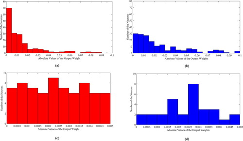
Table 1. Specification of benchmark on regression problems.

Data sets	Training data	Test data	Attributes
Abalone	2000	2177	8.000
Auto price	80.00	79.00	15.00
Boston housing	250.0	256.0	13.00
Machine CPU	100.0	109.0	6.000
Airfoil self-noise	752.0	751.0	6.000
Combined cycle power plant (CCPP)	4784	4784	5.000
Concrete compressive strength (CCS)	515.0	515.0	9.000
Energy efficiency	384.0	384.0	9.000
Gas turbines	5967	5967	14.00
Wine quality	2449	2449	12.00

There are 190 and 184 neurons in the hidden layer, which corresponding absolute values of output weights β fall in the interval (0, 0.1), respectively in I-ELM and II-ELM. From Figure 2(a) and (b), it can be seen that the number of neurons in the hidden layer corresponding to the absolute value of the output weight β of the II-ELM in the interval (0,0.02) is significantly less than that of the I-ELM, while in the interval (0.02,0.1) it is significantly higher than that of the I-ELM. For further comparison, the results of the number of neurons in the hidden layer corresponding to the absolute value of the output weight β of the two models in the interval (0,0.005) are shown in Figure 2(c) and (d). The absolute values of output weights β of the I-ELM and II-ELM in the interval (0, 0.005) correspond to 70 and 30 neurons in the hidden layer, respectively.

According to the above results, the number of invalid neurons in the hidden layer of the II-ELM is significantly smaller than that of the I-ELM after the output offset k is added. The main idea is to find an optimal offset k, and added it to the output vector H of the new added neuron before calculate its weights to the output layer in each training cycle. The optimal offset k can make (8) get minimum value, it means that the residuals error will decline more quickly, and according to (5), the β that closed to zero will be deduced. Therefore II-ELM not only reduces the number of invalid neurons in the I-ELM network, and speeds up the learning speed, but also enhances the stability of the I-ELM network structure and improves the forecasting accuracy.

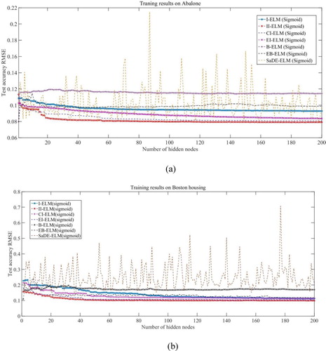
Figure 3 shows the decline curves of the testing error of the network obtained by the I-ELM, II-ELM, CI-ELM, EI-ELM, B-ELM, SaDE-ELM, and EB-ELM with 200 hidden nodes. We suppose ten hidden nodes are randomly generated at each step of the EB-ELM. It can be seen that the learning effect of the II-ELM is much faster than the I-ELM, II-ELM, CI-ELM, EI-ELM, B-ELM, SaDE-ELM, and EB-ELM.

Figure 3. Comparisons between I-ELM network, II-ELM network, CI-ELM network, EI-ELM network, B-ELM network, EB-ELM network, and SaDE-ELM network on Abalone data. (a) Training results on Abalone. (b) Training results on Boston housing.

Tables 2–4 show the training results obtained by the I-ELM, II-ELM, CI-ELM, EI-ELM, B-ELM, SaDE-ELM, EB-ELM, and GA-ELM, respectively. The hidden nodes of them is set to 200. We suppose ten hidden nodes are randomly generated at each step of the EB-ELM. In this paper, the initial values of the parameters of GA are experimentally determined to achieve the best performances, and as follows. The population size is 30, cross probability P_c=0.9, mutation probability P_m=0.01, iteration number of genetic algorithm is 100, root mean square error is 1×10⁻⁵, and using elite strategies (four eligible persons passed directly to the next generation). Average results are collected by the 100 trails for the regression problems under the same experimental conditions. In addition, Tables 2–4 also show the training results of the II-ELM with 30 hidden notes, which is represented as the II-ELM (30).

Table 2. Training time (Second).

	Training time
Data sets	II-ELM (30)	II-ELM	CI-ELM	EI-ELM	B-ELM	SaDE-ELM	I-ELM	EB-ELM	GA-ELM
Abalone	0.0178	0.1126	0.2745	0.2196	0.8862	0.2685	0.0125	0.3864	1.8152
Auto price	0.0065	0.0424	0.7999	0.1245	1.1748	0.7123	0.0345	1.0185	2.2654
Boston housing	0.0103	0.0686	1.1634	0.1554	1.7458	0.8123	0.0525	1.1725	2.3487
Machine CPU	0.0048	0.0325	0.7784	0.1274	1.1901	0.5312	0.0231	0.8245	1.8943
Airfoil self-noise	0.0214	0.0758	0.8561	0.1856	1.2134	0.4231	0.0513	0.8589	1.9654
CCPP	0.1456	0.4861	0.6542	0.5461	2.2145	0.5965	0.4651	2.2131	4.2136
CCS	0.0211	0.0731	0.7895	0.1654	1.0453	0.3154	0.0423	0.7896	1.7652
Energy efficiency	0.0203	0.0689	0.2945	0.0756	1.0321	0.1546	0.0354	0.6321	1.7321
Gas turbines	0.1896	0.7541	2.5541	0.7612	3.214	0.7869	0.5321	2.6123	5.8973
Wine quality	0.1123	0.3451	0.4953	0.3514	2.0165	0.4125	0.2961	1.7541	3.1254

Table 3. Testing RMSE.

	Testing RMSE
Data sets	II-ELM (30)	II-ELM	CI-ELM	EI-ELM	B-ELM	SaDE-ELM	I-ELM	EB-ELM	GA-ELM
Abalone	0.0808	0.0790	0.0825	0.0825	0.0828	4.5394	0.0934	0.0802	0.0797
Auto price	0.1045	0.1004	0.1135	0.1098	0.1142	1.1985	0.1359	0.1035	0.1022
Boston housing	0.1234	0.1074	0.1135	0.1148	0.1192	0.2445	0.1253	0.1091	0.1086
Machine CPU	0.0452	0.0333	0.0399	0.0419	0.0492	19.3175	0.0512	0.0364	0.0354
Airfoil self-noise	0.1398	0.1267	0.1352	0.1379	0.1489	5.6421	0.1575	0.1315	0.1268
CCPP	0.0871	0.0596	0.0615	0.0622	0.0714	5.3214	0.0716	0.0601	0.0594
CCS	0.1654	0.1232	0.1362	0.1364	0.1394	6.2135	0.1412	0.1298	0.1199
Energy efficiency	0.1021	0.0817	0.0844	0.0847	0.0916	5.1234	0.0945	0.0834	0.0821
Gas turbines	0.0321	0.0158	0.0283	0.0295	0.0271	5.2136	0.0312	0.0161	0.0156
Wine quality	0.1454	0.1248	0.1354	0.1354	0.1355	6.2134	0.1358	0.1255	0.1557

Table 4. Standard deviation of testing RMSE.

	Standard deviation of testing RMSE
Data sets	II-ELM (30)	II-ELM	CI-ELM	EI-ELM	B-ELM	SaDE-ELM	I-ELM	EB-ELM	GA-ELM
Abalone	0.0018	0.0005	0.0034	0.0027	0.0023	0.0651	0.0039	0.0016	0.0021
Auto price	0.0085	0.0035	0.0065	0.0059	0.0089	0.4188	0.0078	0.0040	0.0043
Boston housing	0.0073	0.0032	0.0100	0.0047	0.0048	0.0735	0.0177	0.0038	0.0065
Machine CPU	0.0058	0.0041	0.0076	0.0069	0.0059	0.4135	0.0089	0.0049	0.0053
Airfoil self-noise	0.0031	0.0015	0.0035	0.0029	0.0027	0.3421	0.0048	0.0019	0.0014
CCPP	0.0058	0.0016	0.0038	0.0029	0.0023	0.3125	0.0074	0.0016	0.0017
CCS	0.0045	0.0029	0.0056	0.0053	0.0047	0.3654	0.0083	0.0034	0.0039
Energy efficiency	0.0041	0.0021	0.0052	0.0041	0.0039	0.3698	0.0059	0.0026	0.0038
Gas turbines	0.0652	0.0042	0.0083	0.0073	0.0066	0.3541	0.0121	0.0030	0.0055
Wine quality	0.0064	0.0004	0.0021	0.0015	0.0016	0.3145	0.0052	0.0006	0.0008

From Table 2, it is observed that with the same number of the hidden nodes, the rank of the training time in the eight algorithms (I-ELM, II-ELM, CI-ELM, EI-ELM, B-ELM, SaDE-ELM, EB-ELM, and GA-ELM) is: I-ELM < II-ELM < EI-ELM < SaDE-ELM < CI-ELM < EB-ELM < B-ELM < GA-ELM. The reason is that instead of the random generation, the optimization of the hidden neurons in the improved I-ELM always needs the greater computation workloads. But in Table 2, the training time taken by the II-ELM is almost the same as the I-ELM. Compared to other improved I-ELM based methods, the advantage of the II- ELM in the training speed is evident.

From Table 3, it is observed that in the CCPP dataset, CCS dataset, and gas turbines dataset, the rank of the testing RMSE in the eight algorithms(I-ELM, II-ELM, CI-ELM, EI-ELM, B-ELM, SaDE-ELM, EB-ELM, and GA-ELM) is GA-ELM < II-ELM < EB-ELM < CI-ELM < EI-ELM < B-ELM < I-ELM < SaDE-ELM. In the above three datasets, the forecasting accuracy of the II-ELM model and GA-ELM model is very close. In the remaining seven datasets, the rank of the testing RMSE in the eight algorithms(I-ELM, II-ELM, CI-ELM, EI-ELM, B-ELM, SaDE-ELM, EB-ELM, and GA-ELM) is: II-ELM < GA-ELM < EB-ELM < CI-ELM < EI-ELM < B-ELM < I-ELM < SaDE-ELM. The GA-ELM model uses the GA algorithm to optimize the random input weights and thresholds of the ELM model, which greatly improves the accuracy. However it needs to iterate the GA algorithm many times, so that the training time is greatly increased which can be seen from Table 2. Considering the forecasting accuracy and training time of the model, the II-ELM model is superior to the GA-ELM model.

From Table 4, it is observed that with the same number of the hidden nodes, the rank of the standard deviation of the testing RMSE of the I-ELM, II-ELM, CI-ELM, EI-ELM, B-ELM, SaDE-ELM, EB-ELM, and GA-ELM is: II-ELM < EB-ELM < GA-ELM < B-ELM < EI-ELM < I-ELM < CI-ELM < SaDE-ELM. Therefore it can be concluded that compared with the CI-ELM, EI-ELM, B-ELM, SaDE-ELM, EB-ELM, and GA-ELM, the network stability of the II-ELM is higher as well.

From Tables 2–4, the following observation is also made. Comparing the II-ELM algorithm with adding 30 hidden nodes with other algorithms with adding 200 hidden nodes, it is found that the training time of the II-ELM is greatly reduced when the testing RMSE and the standard deviation of the testing RMSE are almost the same as the other algorithms. Thus, the learning speed of the II-ELM algorithm is faster than the CI-ELM, EI-ELM, I-ELM, B-ELM, SaDE-ELM, EB-ELM, and GA-ELM with the same error.

4.2 Classification simulation

Table 5 gives an illustration of the ten real classification problems of the simulations in this paper. Figure 4 shows the rising curves of the classification accuracy of the network obtained by the I-ELM, II-ELM, B-ELM, and SaDE-ELM when adding 200 hidden nodes. It can be seen from Figure 4 that the rising rate of the accuracy in the II-ELM is much faster than the I-ELM, B-ELM, and SaDE-ELM, for both the additive hidden nodes and RBF(the radial basis function) hidden nodes cases.

Figure 4. Comparisons between the I-ELM network, II-ELM network, B-ELM network, and SaDE-ELM network on the Banknote authentication data.

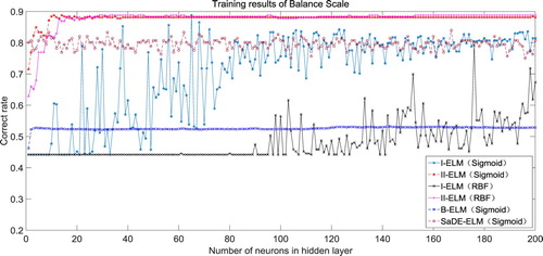
Table 5. Specification of the benchmark on classification problems.

Data sets	Training data	Test data	Attributes
Banknote authentication	686.0	686.0	5.000
Balance scale	313.0	312.0	5.000
Shuttle	7250	7250	10.00
Glass	107.0	107.0	10.00
Blood transfusion service centre	374.0	374.0	5.000
Default of credit card clients	1500	1500	24.00
Diabetic retinopathy debrecen	576.0	575.0	20.00
EEG eye state	7490	7490	15.00
Statlog	2218	2217	37.00
Wine	89.00	89.00	14.00

Table 6 shows the results of the training on the ten real classification problems obtained by the I-ELM and the II-ELM with adding 200 hidden nodes.

Table 6. Correct rate of the classification.

	Sigmoid		RBF
Data sets	II-ELM	I-ELM	II-ELM	I-ELM
Banknote authentication	0.9825	0.6968	0.9810	0.6895
Balance scale	0.8750	0.8109	0.8718	0.8205
Shuttle	0.8599	0.7961	0.8571	0.7966
Glass	0.5794	0.3645	0.5514	0.3645
Blood transfusion service centre	0.7944	0.7848	0.7877	0.7843
Default of credit card clients	0.6123	0.3854	0.6145	0.3862
Diabetic retinopathy debrecen	0.7004	0.5984	0.6506	0.5870
EEG eye state	0.6378	0.3954	0.6437	0.3899
Statlog	0.6473	0.3756	0.6492	0.3741
Wine	0.8348	0.6989	0.7416	0.6652

From Table 6, it is observed that with the same number of the hidden nodes, the accuracy of the classification in the II-ELM is higher than in the I-ELM, for both the additive hidden nodes and the RBF hidden nodes cases.

5. Conclusion

This paper proposes an enhanced algorithm for the I-ELM in which an offset k is added to the output of the hidden nodes, which make the training error of the network reducing more rapidly with the same input weight and bias of the hidden nodes. The algorithm not only improves the training speed of the network, but also improves the testing accuracy. By comparing the performances of the CI-ELM, EI-ELM, B-ELM, SaDE-ELM, EB-ELM, and GA-ELM with the II-ELM on the regression problems, the simulation results show that the II-ELM is better than the CI-ELM, EI-ELM, B-ELM, SaDE-ELM, EB-ELM, and GA-ELM on the learning speed, the network accuracy, and the network stability. By comparing the performances in the II-ELM with I-ELM, B-ELM, and SaDE-ELM, the simulation results demonstrate that the II-ELM is better than the I-ELM, B-ELM, and SaDE-ELM on the classification problems.

However, the II-ELM model proposed in this paper also has certain limitations. The II-ELM model can only reduce invalid neurons in the network and cannot eliminate all invalid neurons, and the input weights and thresholds of the II-ELM model are still obtained randomly. In the next work, the input weights and thresholds of the II-ELM can be further optimized.

Disclosure statement

No potential conflict of interest was reported by the author(s).

Additional information

Funding

This work was supported by the National Natural Science Foundation of China [grant number 51767005]; [Natural Science Foundation of Guangxi Province [grant number 2016GXNSFAA380327].

References

- Cao, W., Gao, J., Wang, X., Ming, Z., & Cai, S. (2020). Random orthogonal projection based enhanced bidirectional extreme learning machine. In J. Cao, C. Vong, Y. Miche, & A. Lendasse (Eds.), Proceedings of ELM 2018. ELM 2018. Proceedings in adaptation, learning and Optimization (vol. 11). Springer. https://doi.org/10.1007/978-3-030-23307-5_1.
- Cao, J., Lin, Z., & Huang, G. (2012). Self-adaptive evolutionary extreme learning machine. Neural Process Letter, 36, 285–305. https://doi.org/10.1007/s11063-012-9236-y
- Cao, W., Ming, Z., Wang, X., & Cai, S. (2019). Improved bidirectional extreme learning machine based on enhanced random search. Memetic Computing, 11(1), 19–26. https://doi.org/10.1007/s12293-017-0238-1
- Cheng, G., Song, S., Lin, Y., Huang, Q., Lin, X., & Wang, F. (2019). Enhanced state estimation and bad data identification in active power distribution networks using photovoltaic power forecasting. Electric Power Systems Research, 177, 105974. https://doi.org/10.1016/j.epsr.2019.105974
- Cui, D., Huang, G. B., & Liu, T. (2018). ELM based smile detection using distance vector. Pattern Recognition, 79, 356–369. https://doi.org/10.1016/j.patcog.2018.02.019
- Huang, G. B. (2015). What are extreme learning machines? Filling the gap between Frank Rosenblatt’s dream and John von Neumann’s puzzle. Cognitive Computation, 7(3), 263–278. https://doi.org/10.1007/s12559-015-9333-0
- Huang, G. B., Bai, Z., Kasun, L. L. C., & Vong, C. M. (2015). Local receptive fields based extreme learning machine. IEEE Computational Intelligence Magazine, 10(2), 18–29. https://doi.org/10.1109/MCI.2015.2405316
- Huang, G. B., & Chen, L. (2007). Convex incremental extreme learning machine. Neurocomputing, 70(16-18), 3056–3062. https://doi.org/10.1016/j.neucom.2007.02.009
- Huang, G. B., & Chen, L. (2008). Enhanced random search based incremental extreme learning machine. Neurocomputing, 71(16-18), 3460–3468. https://doi.org/10.1016/j.neucom.2007.10.008
- Huang, G. B., Chen, L., & Siew, C. K. (2006). Universal approximation using incremental constructive feedforward networks with random hidden nodes. IEEE Transactions on Neural Networks, 17(4), 879–892. https://doi.org/10.1109/TNN.2006.875977
- Huang, G. B., Zhu, Q. Y., & Siew, C. K. (2004, July 25–29). Extreme learning machine: A new learning scheme of feed forward neural networks. 2004 IEEE International Joint Conference on Neural Networks (IEEE Cat. No.04CH37541), Budapest, vol. 2, pp. 985–990. https://doi.org/10.1109/IJCNN.2004.1380068.
- Huang, G. B., Zhu, Q. Y., & Siew, C. K. (2006). Extreme learning machine: Theory and applications. Neurocomputing, 70(1-3), 489–501. https://doi.org/10.1016/j.neucom.2005.12.126
- Inaba, F. K., Teatini Salles, E. O., Perron, S., & Caporossi, G. (2018). DGR-ELM–distributed generalized regularized ELM for classification. Neurocomputing, 275, 1522–1530. https://doi.org/10.1016/j.neucom.2017.09.090
- Li, Q., Han, F., & Ling, Q. (2018). An improved double hidden-layer variable length incremental extreme learning machine based on particle swarm optimization. In D. S. Huang, K. H. Jo, & X. L. Zhang (Eds.), Intelligent computing theories and application. ICIC 2018. Lecture notes in computer science, vol. 10955. Springer. https://doi.org/10.1007/978-3-319-95933-7_5.
- Song, S. J., Wang, Z. H., & Lin, X. F. (2018). Research on SOC estimation of LiFePO_4 batteries based on ELM. Chinese Journal of Power Sources, 42(6), 806–808,881. http://en.cnki.com.cn/Article_en/CJFDTotal-DYJS201806015.htm (in chinese).
- Song, S., Wang, Y., Lin, X., & Huang, Q. (2015, August 26–27). Study on GA-based training algorithm for extreme learning machine. 2015 7th International Conference on Intelligent Human-Machine Systems and Cybernetics, Hangzhou vol. 2, pp. 132–135. https://doi.org/10.1109/IHMSC.2015.156
- Sun, Y., Li, B., Yuan, Y., Bi, X., Zhao, X., & Wang, G. (2019). Big graph classification frameworks based on extreme learning machine. Neurocomputing, 330, 317–327. https://doi.org/10.1016/j.neucom.2018.11.035
- Wang, L., Zeng, Y., & Chen, T. (2015). Back propagation neural network with adaptive differential evolution algorithm for time series forecasting. Expert Systems with Applications, 42(2), 855–863. https://doi.org/10.1016/j.eswa.2014.08.018
- Wu, Y. X., Liu, D., & Jiang, H. (2017). Length-changeable incremental extreme learning machine. Journal of Computer Science and Technology, 32(3), 630–643. https://doi.org/10.1007/s11390-017-1746-7
- Xu, S., & Wang, J. (2016). A fast incremental extreme learning machine algorithm for data streams classification. Expert Systems with Applications, 65, 332–344. https://doi.org/10.1016/j.eswa.2016.08.052
- Yang, A., Li, W., & Yang, X. (2019). Short-term electricity load forecasting based on feature selection and least squares support vector machines. Knowledge-Based Systems, 163, 159–173. https://doi.org/10.1016/j.knosys.2018.08.027
- Yang, Y., Wang, Y., & Yuan, X. (2012). Bidirectional extreme learning machine for regression problem and its learning effectiveness. IEEE Transactions on Neural Networks and Learning Systems, 23(9), 1498–1505. https://doi.org/10.1109/TNNLS.2012.2202289
- Zhang, W., Xu, A., Ping, D., & Gao, M. (2019). An improved kernel-based incremental extreme learning machine with fixed budget for nonstationary time series prediction. Neural Computing and Applications, 31(3), 637–652. https://doi.org/10.1007/s00521-017-3096-3
- Zhao, X. G., Wang, G., Bi, X., Gong, P., & Zhao, Y. (2011). XML document classification based on ELM. Neurocomputing, 74(16), 2444–2451. https://doi.org/10.1016/j.neucom.2010.12.038
- Zhou, Z., Bo, L., Liu, X., Tang, T., & Lv, K. (2019). Fault severity recognition based on self-adaptive particle swarm optimisation using wavelet kernel extreme learning machine. Insight - Non-Destructive Testing and Condition Monitoring, 61(1), 35–43. https://doi.org/10.1784/insi.2019.61.1.35
- Zhou, Z., Chen, J., Song, Y., Zhu, Z., & Liu, X. (2017). RFSEN-ELM: Selective ensemble of extreme learning machines using rotation forest for image classification. Neural Network World, 27(5), 499–517. https://doi.org/10.14311/NNW.2017.27.026
- Zhou, Z., Chen, J., & Zhu, Z. (2018). Regularization incremental extreme learning machine with random reduced kernel for regression. Neurocomputing, 321, 72–81. https://doi.org/10.1016/j.neucom.2018.08.082
- Zhou, Z., Gao, X., Zhang, J., Zhu, Z., & Hu, X. (2019). A novel hybrid model using the rotation forest-based differential evolution online sequential extreme learning machine for illumination correction of dyed fabrics. Textile Research Journal, 89(7), 1180–1197. https://doi.org/10.1177/0040517518764020
- Zhou, Z., Wang, C., Zhang, J., & Zhu, Z. (2020). Color difference classification of solid color printing and dyeing products based on optimization of the extreme learning machine of the improved whale optimization algorithm. Textile Research Journal, 90(2), 135–155. https://doi.org/10.1177/0040517519859933
- Zhou, Z., Wang, C., Zhu, Z., Wang, Y., & Yang, D. (2019). Sliding mode control based on a hybrid grey-wolf-optimized extreme learning machine for robot manipulators. OPTIK, 185, 364–380. https://doi.org/10.1016/j.ijleo.2019.01.105