Statistical accuracy analysis for virtual reference feedback tuning with two degrees of freedom controllers*

Abstract

Virtual reference feedback tuning is one of data-driven control method, as only input–output data are used to design two degrees of freedom controller directly, i.e. feed-forward and feedback controller. Given two desired closed-loop transfer functions, virtual input and virtual disturbance are constructed, respectively to obtain one cost function, whose decision variables correspond to the two unknown controller parameters. Then after formulating the cost function as a linear regression form, the classical least squares algorithm is applied to identify the unknown parameter estimators. To quantify the quality or approximation error of the parameter estimators, statistical accuracy analysis is studied for virtual reference feedback tuning control. The detailed computational process about the asymptotic variance matrix is given by using some knowledge from probability theory and matrix theory. Based on our obtained asymptotic variance matrix, two applications of optimal input design and model structure validation are used to illustrate how to use the obtained asymptotic variance matrix. Finally, one simulation example has been performed to demonstrate the effectiveness of the theories proposed in this paper.

Keywords:

• Virtual reference feedback tuning control
• statistical accuracy analysis
• variance matrix
• application

1. Introduction

For many industrial production processes, safety and production restrictions are often strong reasons for not allowing controller design in an open-loop system. In such situations, it is urgent to design controllers under the closed-loop conditions. When designing controllers in the closed-loop system, only experimental data can be collected about the whole closed-loop system. The main difficulty of designing controller in a closed-loop system is that the researcher must consider the correlation between the reference input and external disturbance, induced by the feedback loop. Consider one problem about how to design controllers in a closed-loop system, a mathematical model about the considered plant must be known in prior. However, the mathematical description or model of the considered plant can not be easily determined in the industrial process, such as paper production factory and other chemical factories.

Virtual reference feedback tuning control is a data-driven control method, where the model identification process can be neglected to simplify the whole design process. In engineering, the classical PID controller is always used to achieve the desired goal. The PID controller is a parametrized controller, so this special parametrized structure is considered in this paper. If the expected controller is parametrized by one unknown parameter vector, the main merits of virtual reference feedback tuning control are to tune the unknown parameter vector in the controller by using only input–output measured data without any knowledge of plant model. So in the idea of virtual reference feedback tuning control, the process of the designing controller is transformed into tuning the unknown parameter vector.

The cost of developing the mathematical model is very high. To avoid the identification process for the plant, one of direct data-driven method-virtual reference feedback tuning control was proposed to design the controller in 1940s (Guardabassi & Savaresi, 2012). The main essence of virtual reference feedback tuning control is that the controller can be designed directly by measured data without any priori knowledge about the plant model. In Bravo et al. (2006), the problem of designing the controller was transformed to identify one unknown parameter vector of the controller. Then the idea of virtual reference feedback tuning control was applied in a benchmark problem (Bravo et al., 2016), where a control cost of the 2-norm type was minimized by using a batch of data collected from the plant. Virtual reference feedback tuning control for controller tuning in a nonlinear setup was introduced in Bravo et al. (2017). In Tanaskovic et al. (2017), the extension of virtual reference feedback tuning control to the the design of two degrees of freedom controller was presented to shape the input–output transfer function of the closed-loop system. As the direct data-driven control approach consists of iterative adjustment of the controller's parameters towards the parameter values, the H2 performance criterion is analysed in order to characterize and enlarge the set of initial parameter values (Campi et al., 2002). The contribution of Campi et al. (2005) introduces an invalidation test step based on the available data to check if the flexibility of the controller parameter is suitable for the design objectives. In recent years, many papers on virtual reference feedback tuning control are published, for example, in Jianhong (2012), the model-matching problems between the closed-loop transfer function and sensitivity function were considered simultaneously, and the iterative sequence generated by the iterative least squares identification algorithm is analysed for identifying the unknown parameter vector. Virtual reference feedback tuning control for constrained closed-loop system was studied in Jianhong (2014b), where the ellipsoid optimization iterative algorithm was adopted to generate a sequence of ellipsoids with decreasing volume. To compromise the gap between the linear and nonlinear controller, the problem of designing a linear time varying controller was solved by using virtual reference feedback tuning control (Jianhong, 2014a). Then through minimizing one approximation error, the adjustable weights in the linear affine function is given in Jianhong (2013). In Jianhong (2017), virtual reference feedback tuning control is combined into internal model control strategy so that the process of identify the plant is avoided in internal model control. In this paper, we do not consider how to design the controller by using virtual reference feedback tuning control, but here we study the finite sample properties of virtual reference feedback tuning with two degrees of freedom control based on a quadratic criterion applied to a simple closed-loop system structure. It is well known that finite sample properties quantitatively assess the discrepancy between minimizing a theoretical identification cost and its empirical counterpart when only a finite number of data points is available (Bazanella et al., 2008). The model quality with many data points is assessed by applying the asymptotic theory under linear model identification condition (Sala & Esparza, 2005). But these asymptotic results hold only when the number of data points tends to infinity (Campi & Savaresi, 2006). Due to the advantage of no identification process, then virtual reference feedback tuning control is more widely applied in engineering and theory research now.

Here in this paper, based on above mentioned references and our previous published contributions (Jianhong, 2012, 2013, 2014a, 2014b, 2017, 2019), we continue to do the deep research on this direct data-driven control strategy-virtual reference feedback tuning control.As in the commonly used closed-loop system, the feed-forward controller and feedback controller exist simultaneously, and these two controllers correspond to the closed-loop system with two degrees of freedom controllers. There are lots of references on designing these two unknown controllers, for the sake of completeness, here classical model reference control and virtual reference feedback tuning control are reviewed. Through comparing the principles between these two strategies, no any priori knowledge about the considered plant is needed in our virtual reference feedback tuning control. Furthermore after constructing the virtual input and virtual disturbance, we find the problem of designing unknown controllers can be changed into one identification problem, whose decision variables are two unknown parameter vectors. Consider the identification with respect to these two unknown parameter vectors, lots of identification algorithms can be applied directly from references, for example, least squares method, separable gradient method, and parallel distributed method, etc. After these two unknown parameter vectors are identified, we need to testify whether our obtained parameter estimators are biased or asymptotic efficient. The whole process to achieve the above goal is named as statistical accuracy analysis for virtual reference feedback tuning control, i.e. probability theory and matrix theory are applied to construct the asymptotic variance matrix for those two unknown parameter vectors. The two diagonal sub-matrices from the asymptotic variance matrix correspond to the asymptotic variance expressions for the unknown parameter vectors. Here we give a more detailed derivation for this complex asymptotic variance matrix through our own mathematical derivations. Based on this obtained asymptotic variance matrix, optimal input design and model structure validation for closed-loop system can be studied. Then the problems about optimal input design and model structure validation are dependent of the obtained asymptotic variance matrix. Generally to quantify the quality of the parameter estimators, statistical accuracy analysis is studied for virtual reference feedback tuning with two degrees of freedom controllers, and the computational process about the asymptotic variance matrix is given more specifically. This asymptotic variance matrix can describe the approximation error between the true value and its estimator. Also from the point of further research on system identification and data-driven control, this obtained asymptotic variance matrix is beneficial for other subjects, such as optimal input design and model structure validation, etc. To pave the road for these other subjects, here some tedious mathematical derivations are given to get that important asymptotic variance matrix. The main contributions of this paper are to derive the asymptotic variance matrix, corresponding to those two unknown controller parameters, and apply this asymptotic variance matrix to optimal input design and model structure validation. To the best of our knowledge that statistical accuracy analysis for virtual reference feedback tuning control is a first work in control research, due to its very strong mathematical basis.

Contributions: Here in this paper, generally the main contributions of this paper are formulated as follow.

1. Derive the asymptotic variance matrix, corresponding to those two unknown controller parameters.

2. Apply this asymptotic variance matrix to optimal input design and model structure validation.

3. Virtual input and virtual disturbance are constructed, respectively to obtain one cost function, which corresponds to two model-matching problems.

4. The classical least squares algorithm is applied to identify the unknown controller parameters on the condition of transforming that cost function as its simplified linear regression form.

The paper is organized as follows. In Section 2, the problem formulation is addressed, and the structure of our considered closed-loop system with two degrees of freedom controllers is presented. To compare virtual reference feedback tuning control and classical model reference control, a short introduction of classical model reference control is given to design the two unknown parametrized controllers in Section 3, and the deficiency of classical model reference control is also pointed out. In Section 4, virtual reference feedback tuning control is proposed to design these two parametrized controllers, furthermore virtual input and virtual disturbance are constructed to get an optimization problem. The simple least squares method and its recursive form are proposed to identify the two unknown parameter vectors in Section 5, and also the detailed process of how to formulate that optimization problem to its simplified form is given. The main contribution about statistical accuracy analysis for virtual reference feedback tuning control is studied in Section 6, some knowledge from probability theory and matrix theory are combined to obtain that important asymptotic variance matrix. Based on this obtained asymptotic variance matrix, its application in optimal input design and model structure validation are described in Section 7. In Section 8, one simulation example illustrates the effectiveness of the proposed theories. Section 9 ends the paper with final conclusion and points out our future work.

2. Problem description

Assume the plant is a linear time invariant discrete time single input and single output process. The plant is denoted by a rational transfer function form $P(z)$, and $P(z)$is unknown. Throughout the closed-loop experimental process, only a sequence of input–output measured data corresponding to the plant $P(z)$ are collected. The input–output relation is described as follows. (1) $y(t)=P(z)u(t)+d(t),$(1) where z is a time shift operator,i.e. $(zu(t)=u(t-1)$, $P(z)$ is one transfer function of the plant, $u(t)$ is the measured input, $y(t)$ is the measured output corresponding to the plant $P(z)$, $d(t)$ is the external noise. When $d(t)$ in Equation (1(1) $y(t)=P(z)u(t)+d(t),$(1) ) is unknown but has known bounds, we regard to the uncertainty associated with $d(t)$ as additive noise because of the way it enters the input–output relation in equation (1(1) $y(t)=P(z)u(t)+d(t),$(1) ).

Consider the following simple closed-loop system with two degrees of freedom controllers in Figure 1, the input–output relations in the whole closed-loop system are written as follows. (2) $\{\begin{array}{l}y(t)=P(z)u(t)+d(t)\\ u(t)=C_1(z,\theta )\epsilon (t)=C_1(z,\theta )[r(t)-C_2(z,\eta )y(t)]\\ \epsilon (t)=r(t)-C_2(z,\eta )y(t)\end{array}$(2) where $r(t)$ is the excited signal, $M(z)$ is one expected transfer function, $C_1(z,\theta )$ and $C_2(z,\eta )$ are two degrees of freedom controllers which are parametrized by the unknown parameter vectors θ and η,respectively, i.e. these two controllers $C_1(z,\theta )$ and $C_2(z,\eta )$ are independently parametrized as the following linear affine forms. (3) $\begin{array}{rl}{C}_1(z,\theta )& ={\alpha }^T(z)\theta ,C_2(z,\eta )={\beta }^T(z)\eta \\ \alpha (z)& =[{\alpha }_1(z),{\alpha }_2(z),\dots ,{\alpha }_n(z){]}^{\mathrm{T}},\\ \beta (z)& =[{\beta }_1(z),{\beta }_2(z),\dots ,{\beta }_n(z){]}^{\mathrm{T}}\\ \theta & =[{\theta }_1,{\theta }_2,\dots ,{\theta }_n{]}^{\mathrm{T}},\eta =[{\eta }_1,{\eta }_2,\dots ,{\eta }_n{]}^{\mathrm{T}},\end{array}$(3) where $\alpha (z)$ and $\beta (z)$ denote two known basic function vectors, θ and β are two unknown parameter vectors with dimension n. One main contribution of this paper is to construct the variance matrix for these two unknown parameter vectors θ and β by using probability theory and matrix theory in the case of probabilistic noise $d(t)$.

Figure 1. The closed-loop system with two degrees of freedom controllers.

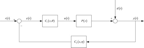
Observing Figure 2, in the classical control system, $C_2(z,\eta )$ is always one sensor, and it sends the output signal back to the input. But in some practical control system such as flight control, vehicle control, etc, $C_2(z,\eta )$ maybe be one feedback controller.

Figure 2. Construction of virtual input.

Formulating Equation (2(2) $\{\begin{array}{l}y(t)=P(z)u(t)+d(t)\\ u(t)=C_1(z,\theta )\epsilon (t)=C_1(z,\theta )[r(t)-C_2(z,\eta )y(t)]\\ \epsilon (t)=r(t)-C_2(z,\eta )y(t)\end{array}$(2) ) again, the new input–output relation in terms of excited input $r(t)$ and external noise $d(t)$ are given as. (4) $\begin{array}{rl}y(t)& =\frac{P(z)C_1(z,\theta )}{1+P(z)C_1(z,\theta )C_2(z,\eta )}r(t)\\ & +\frac{1}{1+P(z)C_1(z,\theta )C_2(z,\eta )}d(t).\end{array}$(4)

3. Classical model reference control

In the closed-loop system with two degrees of freedom controllers, the first transfer function from the excited signal $r(t)$ to measured output $y(t)$ is closed-loop transfer function (Lecchini et al., 2002), and the second transfer function from the external signal $d(t)$ to measured output $y(t)$ is sensitivity function (Milanese & Novara, 2004). From Equation (4(4) $\begin{array}{rl}y(t)& =\frac{P(z)C_1(z,\theta )}{1+P(z)C_1(z,\theta )C_2(z,\eta )}r(t)\\ & +\frac{1}{1+P(z)C_1(z,\theta )C_2(z,\eta )}d(t).\end{array}$(4) ), the control task of classical model reference control is to tune the unknown parameter vectors θ and η corresponding to two degrees of freedom controllers $(C_1(z,\theta ),C_2(z,\eta )$ in order to achieve to the expected closed-loop transfer function and expected sensitivity function. Given the closed-loop transfer function $M(z)$ and expected sensitivity function $S(z)$, we want to guarantee that the closed loop transfer function approximates to its expected function $M(z)$, and the sensitivity function tends to its expected function $S(z)$ too (Alamo et al., 2005). The problem of tuning these two unknown parameter vectors θ and η are formulated as the following classical model reference control optimization problem. (5) $\begin{array}{rl}\underset{\theta ,\eta }{min}{J}_{MR}(\theta ,\eta )& ={\Vert \frac{P(z)C_1(z,\theta )}{1+P(z)C_1(z,\theta )C_2(z,\eta )}-M(z)\Vert }_2^2\\ & +{\Vert \frac{1}{1+P(z)C_1(z,\theta )C_2(z,\eta )}-S(z)\Vert }_2^2\end{array}$(5) where $\Vert \cdot {\Vert }_2^2$ is the common Euclidean norm. In Equation (5(5) $\begin{array}{rl}\underset{\theta ,\eta }{min}{J}_{MR}(\theta ,\eta )& ={\Vert \frac{P(z)C_1(z,\theta )}{1+P(z)C_1(z,\theta )C_2(z,\eta )}-M(z)\Vert }_2^2\\ & +{\Vert \frac{1}{1+P(z)C_1(z,\theta )C_2(z,\eta )}-S(z)\Vert }_2^2\end{array}$(5) ), before solving this optimization problem with respect to unknown parameter vectors θ and η, the priori knowledge about the plant $P(z)$ may be needed. As the plant $P(z)$ is unknown in this model reference control design method, so the identification strategy is used to identify $P(z)$. To avoid the identification process of the plant $P(z)$, virtual reference feedback tuning control is proposed to directly identify the unknown parameter vectors θ and η in two controllers $(C_1(z,\theta ),C_2(z,\eta )$ from the measured input–output data set $Z^N=\{u(t),y(t){\}}_{t=1}^N$, where N is the number of data points.

4. Virtual reference feedback tuning control

Given two controllers $\{(C_1(z,\theta ),C_2(z,\eta ))\}$, as the closed-loop transfer function from $r(t)$ to $y(t)$ is $M(z)$, then we apply one arbitrary signal $r(t)$ to excite the closed-loop system (2(2) $\{\begin{array}{l}y(t)=P(z)u(t)+d(t)\\ u(t)=C_1(z,\theta )\epsilon (t)=C_1(z,\theta )[r(t)-C_2(z,\eta )y(t)]\\ \epsilon (t)=r(t)-C_2(z,\eta )y(t)\end{array}$(2) ), the output of the closed-loop system is described as that. $y(t)=M(z)r(t).$ Consider one special excited input $\overline{r}(t)$, the necessary condition about that the closed-loop transfer function be $M(z)$ is that the two closed-loop systems have the same output $y(t)$ under a given input (Jianhong, 2019). During classical model reference control, this necessary condition holds in case of choosing suitable controller and excited signal. But above description does not hold, due to unknown plant. The idea of virtual reference feedback tuning control means that virtual input $\overline{r}(t)$ and virtual disturbance $\overline{d}(t)$ need to be constructed firstly, so we give the detailed process of constructing virtual input $\overline{r}(t)$ and virtual disturbance $\overline{d}(t)$.

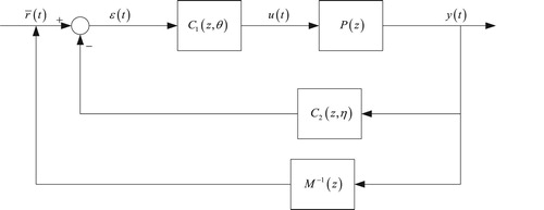
4.1. Virtual input

Collecting input–output sequence $\{u(t),y(t){\}}_{t=1}^N$ of the plant $P(z)$, then for every measured output $y(t)$, define one virtual input $\overline{r}(t)$ such that. (6) $y(t)=M(z)\overline{r}(t).$(6) This virtual input $\overline{r}(t)$ does not exist in reality and it can not be used to generate actual measured output $y(t)$. But virtual input $\overline{r}(t)$ can be obtained by equation $y(t)=M(z)\overline{r}(t)$, i.e. $y(t)$ is the measured output of the closed-loop system, when the excited signal $\overline{r}(t)$ is applied with no disturbance $d(t)=0$.

Due to the unknown plant $P(z)$, and when $P(z)$ is excited by $u(t)$, its output is $y(t)$, so we choose two suitable controllers $\{(C_1(z,\theta ),C_2(z,\eta ))\}$ to obtain one expected signal $u(t)$, if the closed-loop system is excited by virtual input $\overline{r}(t)$ and $y(t)$ simultaneously. The construction of virtual input $\overline{r}(t)$ can be seen Figure 2, where the tracking error $\epsilon (t)$ is defined as. (7) $\begin{array}{rl}\epsilon (t)& =\overline{r}(t)-C_2(z,\eta )y(t)\\ & =(M^{-1}(z)-C_2(z,\eta ))y(t).\end{array}$(7) From Figure 2 we see that when the closed-loop system is excited by $(\overline{r}(t),y(t),d(t)=0)$, the expression of $u(t)$ is get. (8) $\begin{array}{rl}u(t)& =C_1(z,\theta )\epsilon (t)\\ & =C_1(z,\theta )(M^{-1}(z)-C_2(z,\eta ))y(t).\end{array}$(8)

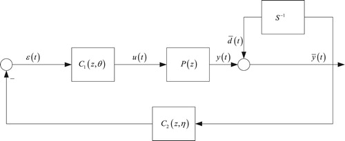
4.2. Virtual disturbance

Given the measured output $y(t)$, define one virtual disturbance $\overline{d}(t)$ to guarantee that when the closed-loop system is excited by virtual disturbance $\overline{d}(t)$, the obtained output $\overline{y}(t)$ is defined as that. (9) $\overline{y}(t)=y(t)+\overline{d}(t).$(9) The construction of virtual disturbance $\overline{d}(t)$ is in Figure 3, where this virtual disturbance $\overline{d}(t)$ satisfied that. (10) $y(t)+\overline{d}(t)=S(z)\overline{d}(t).$(10) Equation (10(10) $y(t)+\overline{d}(t)=S(z)\overline{d}(t).$(10) ) is used to generate virtual disturbance $\overline{d}(t)$, it means that when the closed-loop system is excited by the following signals $(r(t)=0,\overline{d}(t),\overline{y}(t)=y(t)+\overline{d}(t)$, the obtained sinal $u(t)$ is get. (11) $u(t)=-C_1(z,\theta )C_2(z,\eta )\overline{y}(t).$(11) As $\overline{y}(t)$ in Equation (11(11) $u(t)=-C_1(z,\theta )C_2(z,\eta )\overline{y}(t).$(11) ) is not the true output, and instead the true output is $y(t)$, so $\overline{y}(t)$ in Equation (11(11) $u(t)=-C_1(z,\theta )C_2(z,\eta )\overline{y}(t).$(11) ) must be changed into $y(t)$.

Figure 3. Construction of virtual disturbance.

Combining two equations (9(9) $\overline{y}(t)=y(t)+\overline{d}(t).$(9) ) and (11(11) $u(t)=-C_1(z,\theta )C_2(z,\eta )\overline{y}(t).$(11) ), we get that. (12) $y(t)=(S(z)-1)\overline{d}(t)=(S(z)-1)S^{-1}(z)\overline{y}(t).$(12) Furthermore we have. (13) $\overline{y}(t)=\frac{S(z)}{S(z)-1}y(t).$(13) Using equations (8(8) $\begin{array}{rl}u(t)& =C_1(z,\theta )\epsilon (t)\\ & =C_1(z,\theta )(M^{-1}(z)-C_2(z,\eta ))y(t).\end{array}$(8) ) and (13(13) $\overline{y}(t)=\frac{S(z)}{S(z)-1}y(t).$(13) ), two unknown parameter vectors θ and η in two controllers $\{(C_1(z,\theta ),C_2(z,\eta ))\}$ can be identified by solving the following optimization problem. (14) $\begin{array}{rl}& \underset{\theta ,\eta }{min}{J}_{VR}^N(\theta ,\eta )\\ & =\frac{1}{N}\sum _{t=1}^N[u(t)-C_1(z,\theta )(M^{-1}(z)-C_2(z,\eta ))y(t){]}^2\\ & +\frac{1}{N}\sum _{t=1}^N{[u(t)+C_1(z,\theta )C_2(z,\eta )\frac{S(z)}{S(z)-1}y(t)]}^2\end{array}$(14) Observing optimization problem (14(14) $\begin{array}{rl}& \underset{\theta ,\eta }{min}{J}_{VR}^N(\theta ,\eta )\\ & =\frac{1}{N}\sum _{t=1}^N[u(t)-C_1(z,\theta )(M^{-1}(z)-C_2(z,\eta ))y(t){]}^2\\ & +\frac{1}{N}\sum _{t=1}^N{[u(t)+C_1(z,\theta )C_2(z,\eta )\frac{S(z)}{S(z)-1}y(t)]}^2\end{array}$(14) ), all variables are known except for two parametrized controllers $\{(C_1(z,\theta ),C_2(z,\eta ))\}$. More specifically, input–output data $\{u(t),y(t){\}}_{t=1}^N$ can be collected by sensors, these two expected transfer functions $M(z)$ and $S(z)$ are priori known. Roughly speaking, the plant $P(z)$ is not in optimization problem (14(14) $\begin{array}{rl}& \underset{\theta ,\eta }{min}{J}_{VR}^N(\theta ,\eta )\\ & =\frac{1}{N}\sum _{t=1}^N[u(t)-C_1(z,\theta )(M^{-1}(z)-C_2(z,\eta ))y(t){]}^2\\ & +\frac{1}{N}\sum _{t=1}^N{[u(t)+C_1(z,\theta )C_2(z,\eta )\frac{S(z)}{S(z)-1}y(t)]}^2\end{array}$(14) ), which is the main contribution in virtual reference feedback tuning control. Furthermore optimization problem (14(14) $\begin{array}{rl}& \underset{\theta ,\eta }{min}{J}_{VR}^N(\theta ,\eta )\\ & =\frac{1}{N}\sum _{t=1}^N[u(t)-C_1(z,\theta )(M^{-1}(z)-C_2(z,\eta ))y(t){]}^2\\ & +\frac{1}{N}\sum _{t=1}^N{[u(t)+C_1(z,\theta )C_2(z,\eta )\frac{S(z)}{S(z)-1}y(t)]}^2\end{array}$(14) ) embodied that the problem of designing two controllers can be transformed to identify two unknown parameter vectors. This transformation will simplify the latter computational complexity for designing controllers.

5. Identification algorithm

From above descriptions on virtual reference feedback tuning, the main step is to identify two unknown parameter vectors $(\theta ,\eta )$. But now lots of identification algorithms proposed in references are based on probability distribution on external disturbance (Weyer, 2000). Generally to validate the applied model in engineering, some uncertainties can be added to the mathematical model. Frequently disturbance inflecting the real system has to be taken into account in the mathematical model in order to ensure a similar behaviour of the real system and the mathematical model. Here the main contribution is about statistical accuracy analysis on virtual reference feedback tuning control, not on the identification algorithm, so for the sale of completeness, here in this section we only use the simple least squares algorithm to identify those two unknown parameter vectors $(\theta ,\eta )$. In order to apply the classical least squares algorithm, from the theoretical perspective, firstly we transform the problem of identifying unknown parameter vectors in virtual reference feedback tuning control into two linear regression models,which are suitable for least squares algorithm algorithm.

Observing the optimization problem (14(14) $\begin{array}{rl}& \underset{\theta ,\eta }{min}{J}_{VR}^N(\theta ,\eta )\\ & =\frac{1}{N}\sum _{t=1}^N[u(t)-C_1(z,\theta )(M^{-1}(z)-C_2(z,\eta ))y(t){]}^2\\ & +\frac{1}{N}\sum _{t=1}^N{[u(t)+C_1(z,\theta )C_2(z,\eta )\frac{S(z)}{S(z)-1}y(t)]}^2\end{array}$(14) ) in virtual reference feedback tuning control, our goal is to identify two optimal parameter vectors such that the above forms hold. Let (15) $\begin{array}{rl}& C_1(z,\theta )(M^{-1}(z)-C_2(z,\eta ))y(t)\\ & =-C_1(z,\theta )C_2(z,\eta )\frac{S(z)}{S(z)-1}y(t).\end{array}$(15) Then (16) $(M^{-1}(z)-C_2(z,\eta )+C_2(z,\eta )\frac{S(z)}{S(z)-1})y(t)=0.$(16) It means that (17) $\{\begin{array}{l}((S(z)-1)M^{-1}(z)+C_2(z,\eta ))y(t)=0\\ C_2(z,\eta )y(t)-(S(z)-1)M^{-1}(z)y(t)=0\end{array}$(17) Using the Equation (3(3) $\begin{array}{rl}{C}_1(z,\theta )& ={\alpha }^T(z)\theta ,C_2(z,\eta )={\beta }^T(z)\eta \\ \alpha (z)& =[{\alpha }_1(z),{\alpha }_2(z),\dots ,{\alpha }_n(z){]}^{\mathrm{T}},\\ \beta (z)& =[{\beta }_1(z),{\beta }_2(z),\dots ,{\beta }_n(z){]}^{\mathrm{T}}\\ \theta & =[{\theta }_1,{\theta }_2,\dots ,{\theta }_n{]}^{\mathrm{T}},\eta =[{\eta }_1,{\eta }_2,\dots ,{\eta }_n{]}^{\mathrm{T}},\end{array}$(3) ) as. (18) $C_2(z,\eta )={\beta }^T(z)\eta =[1z{z}^2\dots z^n]\left[\begin{array}{c}1\\ {\eta }_1\\ {\eta }_2\\ ⋮\\ {\eta }_n\end{array}\right]$(18) Substituting the above linear affine form (3(3) $\begin{array}{rl}{C}_1(z,\theta )& ={\alpha }^T(z)\theta ,C_2(z,\eta )={\beta }^T(z)\eta \\ \alpha (z)& =[{\alpha }_1(z),{\alpha }_2(z),\dots ,{\alpha }_n(z){]}^{\mathrm{T}},\\ \beta (z)& =[{\beta }_1(z),{\beta }_2(z),\dots ,{\beta }_n(z){]}^{\mathrm{T}}\\ \theta & =[{\theta }_1,{\theta }_2,\dots ,{\theta }_n{]}^{\mathrm{T}},\eta =[{\eta }_1,{\eta }_2,\dots ,{\eta }_n{]}^{\mathrm{T}},\end{array}$(3) ) of the parametrized controller $C_2(z,\eta )$ into above Equation (17(17) $\{\begin{array}{l}((S(z)-1)M^{-1}(z)+C_2(z,\eta ))y(t)=0\\ C_2(z,\eta )y(t)-(S(z)-1)M^{-1}(z)y(t)=0\end{array}$(17) ), then we have. (19) $[1z{z}^2\dots z^n]\left[\begin{array}{c}1\\ {\eta }_1\\ {\eta }_2\\ ⋮\\ {\eta }_n\end{array}\right]y(t)=(S(z)-1)M^{-1}(z)y(t),$(19) where one special basic function vector is used here. $\alpha (z)=\beta (z)=[1z{z}^2\dots z^n{]}^{\mathrm{T}}$ Rewriting above Equation (19(19) $[1z{z}^2\dots z^n]\left[\begin{array}{c}1\\ {\eta }_1\\ {\eta }_2\\ ⋮\\ {\eta }_n\end{array}\right]y(t)=(S(z)-1)M^{-1}(z)y(t),$(19) ) as one linear regression model. $\begin{array}{rl}y(t)& =y(t-1){\eta }_1+y(t-2){\eta }_2+\cdots +y(t-n){\eta }_n\\ & +(S(z)-1)M^{-1}(z)y(t).\end{array}$ Hence (20) $\begin{array}{rl}y(t)& =\frac{M(z)}{M(z)-S(z)+1}\\ & \times [y(t-1)y(t-2)\dots y(t-n)]\left[\begin{array}{c}{\eta }_1\\ {\eta }_2\\ ⋮\\ {\eta }_n\end{array}\right]\end{array}$(20) Introduce the regression vector $\varphi (t)$ as that. $\begin{array}{rl}\varphi (t)& =\frac{M(z)}{M(z)-S(z)+1}\\ & \times [y(t-1)y(t-2)\dots y(t-n)]\end{array}$ Then Equation (19(19) $[1z{z}^2\dots z^n]\left[\begin{array}{c}1\\ {\eta }_1\\ {\eta }_2\\ ⋮\\ {\eta }_n\end{array}\right]y(t)=(S(z)-1)M^{-1}(z)y(t),$(19) ) will be a linear regression model. (21) $y(t)=\varphi (t{)}^T\eta$(21) After the unknown parameter vector η is identified and substituting its estimator $\hat{\eta }$ into the parametrized controller, then controller $C_2(z,\hat{\eta })$ is obtained. Applying this obtained controller $C_2(z,\hat{\eta })$ into equation (17(17) $\{\begin{array}{l}((S(z)-1)M^{-1}(z)+C_2(z,\eta ))y(t)=0\\ C_2(z,\eta )y(t)-(S(z)-1)M^{-1}(z)y(t)=0\end{array}$(17) ), then we have. (22) $\begin{array}{rl}u(t)& =-C_1(z,\theta )C_2(z,\hat{\eta })\frac{S(z)}{S(z)-1}y(t)\\ & =-\frac{S(z)C_2(z,\hat{\eta })}{S(z)-1}y(t)[1z{z}^2\dots z^n]\left[\begin{array}{c}1\\ {\theta }_1\\ {\theta }_2\\ ⋮\\ {\theta }_n\end{array}\right]\end{array}$(22) Similarly based on that special basic function vector $\alpha (z)$, Equation (22(22) $\begin{array}{rl}u(t)& =-C_1(z,\theta )C_2(z,\hat{\eta })\frac{S(z)}{S(z)-1}y(t)\\ & =-\frac{S(z)C_2(z,\hat{\eta })}{S(z)-1}y(t)[1z{z}^2\dots z^n]\left[\begin{array}{c}1\\ {\theta }_1\\ {\theta }_2\\ ⋮\\ {\theta }_n\end{array}\right]\end{array}$(22) ) can be also written as another linear regression model. (23) $u(t)=\phi (t{)}^T\theta ,$(23) where the regressor vector $\phi (t)$ is defined as. $\phi (t)=-\frac{S(z)C_2(z,\hat{\eta })}{S(z)-1}y(t)[1z{z}^2\dots z^n]$ From these two linear regression models (21(21) $y(t)=\varphi (t{)}^T\eta$(21) ) and (23(23) $u(t)=\phi (t{)}^T\theta ,$(23) ), we see that firstly the unknown parameter vector η can be identified on basis of linear regression model (21(21) $y(t)=\varphi (t{)}^T\eta$(21) ), then after substituting its estimator $\hat{\eta }$ into the regressor vector $\alpha (z)$, another unknown parameter vector θ is obtained from linear regression model (23(23) $u(t)=\phi (t{)}^T\theta ,$(23) ). So here we only give a detailed least squares identification algorithm to identify the unknown parameter vector η in linear regression model (23(23) $u(t)=\phi (t{)}^T\theta ,$(23) ), the identification of θ is similar to our derivation.

Observing that linear regression model (21(21) $y(t)=\varphi (t{)}^T\eta$(21) ) with respect to unknown parameter vector η, its least squares algorithm is easily used here, i.e. (24) $\hat{\eta }={[\sum _{t=1}^N\varphi (t){\varphi }^T(t)]}^{-1}[\sum _{t=1}^N\varphi (t)y(t)]$(24) Also its general recursive least squares algorithm is given as. (25) $\begin{array}{rl}\hat{\eta }(t)& =\hat{\eta }(t-1)+g(t)[y(t)-{\varphi }^T(t)\hat{\eta }(t-1)]\\ g(t)& =P(t-1)\varphi (t)[1+{\varphi }^T(t)P(t-1)\varphi (t){]}^{-1}\\ P(t)& =P(t-1)-g(t){\varphi }^T(t)P(t-1),\end{array}$(25) where $\hat{\eta }(t)$ denotes the parameter estimator at iterative step t, and $g(t)$ is one gain matrix. Furthermore recursive form (25(25) $\begin{array}{rl}\hat{\eta }(t)& =\hat{\eta }(t-1)+g(t)[y(t)-{\varphi }^T(t)\hat{\eta }(t-1)]\\ g(t)& =P(t-1)\varphi (t)[1+{\varphi }^T(t)P(t-1)\varphi (t){]}^{-1}\\ P(t)& =P(t-1)-g(t){\varphi }^T(t)P(t-1),\end{array}$(25) ) can be written in the following simplified form. (26) $\hat{\eta }(t)=\hat{\eta }(t-1)+P(t)\varphi (t)[y(t)-{\varphi }^T(t)\hat{\eta }(t-1)].$(26) This above alternative expression will be useful in the subsequent analysis.

To make the above recursive form hold and retain the convergence of the above least squares algorithm, one condition is needed to guarantee that inverse matrix $\varphi (t){\varphi }^T(t)$ exist, roughly speaking, this condition corresponds to the persistent excitation, that is described as follows in detail.

Remark

Persistence of excitation

The regression vector $\varphi (t)$ is persistent excitation with a level of excitation ${\alpha }_0>0$, if there exist constant ${\alpha }_1>0$, such that. ${\alpha }_{0}I\le [\sum _{t=1}^N\varphi (t){\varphi }^T(t)]\le {\alpha }_{1}I,\mathrm{\forall }t\ge 0,$ where I is one unit matrix.

The above inequality means matrix $\varphi (t){\varphi }^T(t)$ is non-singular for all t, the concept of persistent excitation requires that $\varphi (t)$ varies in such a way with time, that the sum of the matrix $\varphi (t){\varphi }^T(t)$ is uniformly positive definite over any time instant $t=1,2\dots N$.

6. Statistical accuracy analysis

Accuracy analysis is one important factor in system identification and parameter estimation theory, as it can not only show the accuracy property for the parameter estimator, but also provide one useful tool to other research fields, such as optimal input design and model structure validation, etc. Two statistical variables are always used in accuracy analysis, i.e. expectation and variance, as variance can measure the approximation error between the true value and its estimator. If the approximation error is not tolerable, it means the parameter estimator is biased, and the whole process of system identification must be repeated until to obtain one unbiased estimator. The main contribution of this section is to derive the variance matrix for those two unknown parameter vectors $(\theta ,\eta )$ through our own mathematical derivation.

Observing that optimization problem (14(14) $\begin{array}{rl}& \underset{\theta ,\eta }{min}{J}_{VR}^N(\theta ,\eta )\\ & =\frac{1}{N}\sum _{t=1}^N[u(t)-C_1(z,\theta )(M^{-1}(z)-C_2(z,\eta ))y(t){]}^2\\ & +\frac{1}{N}\sum _{t=1}^N{[u(t)+C_1(z,\theta )C_2(z,\eta )\frac{S(z)}{S(z)-1}y(t)]}^2\end{array}$(14) ) and applying the collected data set $Z^N=\{u(t),y(t){\}}_{t=1}^N$, where N is the number of total data points. Two unknown parameter vectors $(\theta ,\eta )$ are identified by solving the following optimization problem. (27) $({\hat{\theta }}_N,{\hat{\eta }}_N)=\underset{(\theta ,\eta )}{\arg min}{J}_{VR}^N(\theta ,\eta ).$(27) Then the asymptotic estimators are derived as the following limit form. (28) $({\theta }^{\ast },{\eta }^{\ast })=\underset{(\theta ,\eta )}{\arg min}\underset{N\to \mathrm{\infty }}{lim}E{J}_{VR}^N(\theta ,\eta ),$(28) where E is the expectation operation, and $E{J}_{VR}^N(\theta ,\eta )$ is rewritten as. (29) $\begin{array}{rl}E{J}_{VR}^N(\theta ,\eta )& =E[M_1(z)u(t)-C_1(z,\theta )y(t)\\ & +M_1(z)C_1(z,\theta )C_2(z,\eta )y(t){]}^2\\ & +E[u(t)+C_1(z,\theta )C_2(z,\eta )M_2(z)y(t){]}^2,\end{array}$(29) where $M_1(z)$ and $M_2(z)$ are defined as $\begin{array}{rl}{M}_1(z)& =M(z),\\ M_2(z)& =\frac{S(z)}{S(z)-1}.\end{array}$ From the point of probability theory (Campi & Weyer, 2002), the following asymptotic relations hold on the condition of $N\to \mathrm{\infty }$. (30) $\begin{array}{rl}{J}_{VR}^N(\theta ,\eta )& \to J_{VR}(\theta ,\eta )=E{J}_{VR}^N(\theta ,\eta ),\\ ({\hat{\theta }}_N,{\hat{\eta }}_N)& \to ({\theta }^{\ast },{\eta }^{\ast }),N\to \mathrm{\infty }.\end{array}$(30) Using the first order optimal necessary condition, if $({\hat{\theta }}_N,{\hat{\eta }}_N)$ and $({\theta }^{\ast },{\eta }^{\ast })$ are minimal values for their own cost functions,respectively, the following relations hold. (31) $\begin{array}{rl}{\left[\frac{\mathrm{\partial }{J}_{VR}^N(\theta ,\eta )}{\mathrm{\partial }\theta }\right]}_{({\hat{\theta }}_N,{\hat{\eta }}_N)}& =0;{\left[\frac{\mathrm{\partial }{J}_{VR}(\theta ,\eta )}{\mathrm{\partial }\theta }\right]}_{({\theta }^{\ast },{\eta }^{\ast })}=0,\end{array}$(31) (32) $\begin{array}{rl}{\left[\frac{\mathrm{\partial }{J}_{VR}^N(\theta ,\eta )}{\mathrm{\partial }\eta }\right]}_{({\hat{\theta }}_N,{\hat{\eta }}_N)}& =0;{\left[\frac{\mathrm{\partial }{J}_{VR}(\theta ,\eta )}{\mathrm{\partial }\eta }\right]}_{({\theta }^{\ast },{\eta }^{\ast })}=0.\end{array}$(32) Expanding the above equations with respect to θ, then we get. (33) $\begin{array}{rl}& \frac{2}{N}\sum _{t=1}^N[M_1(z)u(t)-C_1(z,\theta )y(t)\\ & +M_1(z)C_1(z,\theta )C_2(z,\eta )y(t)]\\ & \times [-\frac{\mathrm{\partial }{C}_1(z,\theta )}{\mathrm{\partial }\theta }y(t)+M_1(z)\frac{\mathrm{\partial }{C}_1(z,\theta )}{\mathrm{\partial }\theta }{C}_2(z,\eta )y(t)]\\ & +\frac{2}{N}\sum _{t=1}^N[u(t)+C_1(z,\theta )C_2(z,\eta )M_2(z)y(t)]\\ & \times [\frac{\mathrm{\partial }{C}_1(z,\theta )}{\mathrm{\partial }\theta }{C}_2(z,\eta )M_2(z)y(t)]=0.\end{array}$(33) Similarly expanding the above equations with respect to η, then we get. (34) $\begin{array}{rl}& \frac{2}{N}\sum _{t=1}^N[M_1(z)u(t)-C_1(z,\theta )y(t)\\ & +M_1(z)C_1(z,\theta )C_2(z,\eta )y(t)]\\ & \times [M_1(z)C_1(z,\theta )\frac{\mathrm{\partial }{C}_2(z,\eta )}{\mathrm{\partial }\eta }y(t)]\\ & +\frac{2}{N}\sum _{t=1}^N[u(t)+C_1(z,\theta )C_2(z,\eta )M_2(z)y(t)]\\ & \times [\frac{\mathrm{\partial }{C}_2(z,\eta )}{\mathrm{\partial }\eta }{C}_1(z,\theta )M_2(z)y(t)]=0.\end{array}$(34) Let $\xi =(\theta ,\eta )$, then above two equations are rewritten as. (35) $\begin{array}{rl}{\hat{\xi }}_N& =({\hat{\theta }}_N,{\hat{\eta }}_N)={\arg min}_{\xi =(\theta ,\eta )}{J}_{VR}^N(\xi )\\ & ={\arg min}_{\xi =(\theta ,\eta )}{J}_{VR}^N(\theta ,\eta )\\ {\xi }^{\ast }& =({\theta }^{\ast },{\eta }^{\ast })={\arg min}_{\xi =(\theta ,\eta )}{J}_{VR}(\xi )\\ & ={\arg min}_{\xi =(\theta ,\eta )}{J}_{VR}(\theta ,\eta )\end{array}$(35) (36) ${\left[\frac{\mathrm{\partial }{J}_{VR}^N(\xi )}{\mathrm{\partial }\xi }\right]}_{{\hat{\xi }}_N}={\left[\begin{array}{c}{\displaystyle \frac{\mathrm{\partial }{J}_{VR}^N(\xi )}{\mathrm{\partial }\theta }}\\ {\displaystyle \frac{\mathrm{\partial }{J}_{VR}^N(\xi )}{\mathrm{\partial }\eta }}\end{array}\right]}_{{\hat{\xi }}_N=({\hat{\theta }}_N,{\hat{\eta }}_N)}=0.$(36) Using Taylor series expansion formula, the first order partial derivative can be expanded around the asymptotic limit point ${\xi }^{\ast }=({\theta }^{\ast },{\eta }^{\ast })$, i.e. (37) $\begin{array}{rl}{\left[\frac{\mathrm{\partial }{J}_{VR}^N(\xi )}{\mathrm{\partial }\xi }\right]}_{{\hat{\xi }}_N}& ={\left[\frac{\mathrm{\partial }{J}_{VR}^N(\xi )}{\mathrm{\partial }\xi }\right]}_{{\xi }^{\ast }}\\ & +{\left[\frac{{\mathrm{\partial }}^2{J}_{VR}^N(\xi )}{\mathrm{\partial }{\xi }^2}\right]}_{{\xi }^{\ast }}({\hat{\xi }}_N-{\xi }^{\ast }).\end{array}$(37) Expanding above equation to get. (38) $\begin{array}{rl}\left[\begin{array}{c}0\\ 0\end{array}\right]& ={\left[\begin{array}{c}{\displaystyle \frac{\mathrm{\partial }{J}_{VR}^N(\xi )}{\mathrm{\partial }\theta }}\\ {\displaystyle \frac{\mathrm{\partial }{J}_{VR}^N(\xi )}{\mathrm{\partial }\eta }}\end{array}\right]}_{{\xi }^{\ast }}\\ & +{\left[\begin{array}{c}{\displaystyle \frac{{\mathrm{\partial }}^2{J}_{VR}^N(\xi )}{\mathrm{\partial }{\theta }^2}}\\ {\displaystyle \frac{{\mathrm{\partial }}^2{J}_{VR}^N(\xi )}{\mathrm{\partial }{\eta }^2}}\end{array}\right]}_{{\xi }^{\ast }}\left[\begin{array}{c}{\hat{\theta }}_N-{\theta }^{\ast }\\ {\hat{\eta }}_N-{\eta }^{\ast }\end{array}\right]\end{array}$(38) Observing Equation (37(37) $\begin{array}{rl}{\left[\frac{\mathrm{\partial }{J}_{VR}^N(\xi )}{\mathrm{\partial }\xi }\right]}_{{\hat{\xi }}_N}& ={\left[\frac{\mathrm{\partial }{J}_{VR}^N(\xi )}{\mathrm{\partial }\xi }\right]}_{{\xi }^{\ast }}\\ & +{\left[\frac{{\mathrm{\partial }}^2{J}_{VR}^N(\xi )}{\mathrm{\partial }{\xi }^2}\right]}_{{\xi }^{\ast }}({\hat{\xi }}_N-{\xi }^{\ast }).\end{array}$(37) ) again, the following relation holds. (39) $\begin{array}{rl}({\hat{\xi }}_N-{\xi }^{\ast })& =-{\left[\begin{array}{cc}{\displaystyle \frac{{\mathrm{\partial }}^2{J}_{VR}^N(\xi )}{\mathrm{\partial }{\theta }^2}}& {\displaystyle \frac{{\mathrm{\partial }}^2{J}_{VR}^N(\xi )}{\mathrm{\partial }\theta \mathrm{\partial }\eta }}\\ {\displaystyle \frac{{\mathrm{\partial }}^2{J}_{VR}^N(\xi )}{\mathrm{\partial }\theta \mathrm{\partial }\eta }}& {\displaystyle \frac{{\mathrm{\partial }}^2{J}_{VR}^N(\xi )}{\mathrm{\partial }{\eta }^2}}\end{array}\right]}^{-1}\\ & \times \left[\begin{array}{c}{\displaystyle \frac{\mathrm{\partial }{J}_{VR}^N(\xi )}{\mathrm{\partial }\theta }}\\ {\displaystyle \frac{\mathrm{\partial }{J}_{VR}^N(\xi )}{\mathrm{\partial }\eta }}\end{array}\right]\end{array}$(39) From Equation (39(39) $\begin{array}{rl}({\hat{\xi }}_N-{\xi }^{\ast })& =-{\left[\begin{array}{cc}{\displaystyle \frac{{\mathrm{\partial }}^2{J}_{VR}^N(\xi )}{\mathrm{\partial }{\theta }^2}}& {\displaystyle \frac{{\mathrm{\partial }}^2{J}_{VR}^N(\xi )}{\mathrm{\partial }\theta \mathrm{\partial }\eta }}\\ {\displaystyle \frac{{\mathrm{\partial }}^2{J}_{VR}^N(\xi )}{\mathrm{\partial }\theta \mathrm{\partial }\eta }}& {\displaystyle \frac{{\mathrm{\partial }}^2{J}_{VR}^N(\xi )}{\mathrm{\partial }{\eta }^2}}\end{array}\right]}^{-1}\\ & \times \left[\begin{array}{c}{\displaystyle \frac{\mathrm{\partial }{J}_{VR}^N(\xi )}{\mathrm{\partial }\theta }}\\ {\displaystyle \frac{\mathrm{\partial }{J}_{VR}^N(\xi )}{\mathrm{\partial }\eta }}\end{array}\right]\end{array}$(39) ). the asymptotic result corresponding to the unknown parameter vector ξ is derived as follows. (40) $\sqrt{N}({\hat{\xi }}_N-{\xi }^{\ast })\to \mathcal{N}(0,A),\mathrm{as}N\to \mathrm{\infty },$(40) where $\mathcal{N}(0,A)$ denotes one normal distribution with zero mean and variance matrix A. Equation (40(40) $\sqrt{N}({\hat{\xi }}_N-{\xi }^{\ast })\to \mathcal{N}(0,A),\mathrm{as}N\to \mathrm{\infty },$(40) ) tells us that the parameter estimator ${\hat{\xi }}_N$ converges to its true asymptotic limit value ${\xi }^{\ast }$, and the approximation error approaches to one Gaussian stochastic variable. Its asymptotic variance matrix A is defined as follows. (41) $\begin{array}{rl}A& =\left[\begin{array}{cc}{A}_{\theta }& A_{\theta \eta }\\ A_{\theta \eta }& A_{\eta }\end{array}\right]\\ & ={\left[\begin{array}{cc}{\displaystyle \frac{{\mathrm{\partial }}^2{J}_{VR}^N(\xi )}{\mathrm{\partial }{\theta }^2}}& {\displaystyle \frac{{\mathrm{\partial }}^2{J}_{VR}^N(\xi )}{\mathrm{\partial }\theta \mathrm{\partial }\eta }}\\ {\displaystyle \frac{{\mathrm{\partial }}^2{J}_{VR}^N(\xi )}{\mathrm{\partial }\theta \mathrm{\partial }\eta }}& {\displaystyle \frac{{\mathrm{\partial }}^2{J}_{VR}^N(\xi )}{\mathrm{\partial }{\eta }^2}}\end{array}\right]}^{-1}\mathrm{cov}\left[\begin{array}{c}{\displaystyle \frac{\mathrm{\partial }{J}_{VR}^N(\xi )}{\mathrm{\partial }\theta }}\\ {\displaystyle \frac{\mathrm{\partial }{J}_{VR}^N(\xi )}{\mathrm{\partial }\eta }}\end{array}\right]\\ & \times {\left[\begin{array}{cc}{\displaystyle \frac{{\mathrm{\partial }}^2{J}_{VR}^N(\xi )}{\mathrm{\partial }{\theta }^2}}& {\displaystyle \frac{{\mathrm{\partial }}^2{J}_{VR}^N(\xi )}{\mathrm{\partial }\theta \mathrm{\partial }\eta }}\\ {\displaystyle \frac{{\mathrm{\partial }}^2{J}_{VR}^N(\xi )}{\mathrm{\partial }\theta \mathrm{\partial }\eta }}& {\displaystyle \frac{{\mathrm{\partial }}^2{J}_{VR}^N(\xi )}{\mathrm{\partial }{\eta }^2}}\end{array}\right]}^{-\mathrm{T}}\end{array}$(41) Above Equation (41(41) $\begin{array}{rl}A& =\left[\begin{array}{cc}{A}_{\theta }& A_{\theta \eta }\\ A_{\theta \eta }& A_{\eta }\end{array}\right]\\ & ={\left[\begin{array}{cc}{\displaystyle \frac{{\mathrm{\partial }}^2{J}_{VR}^N(\xi )}{\mathrm{\partial }{\theta }^2}}& {\displaystyle \frac{{\mathrm{\partial }}^2{J}_{VR}^N(\xi )}{\mathrm{\partial }\theta \mathrm{\partial }\eta }}\\ {\displaystyle \frac{{\mathrm{\partial }}^2{J}_{VR}^N(\xi )}{\mathrm{\partial }\theta \mathrm{\partial }\eta }}& {\displaystyle \frac{{\mathrm{\partial }}^2{J}_{VR}^N(\xi )}{\mathrm{\partial }{\eta }^2}}\end{array}\right]}^{-1}\mathrm{cov}\left[\begin{array}{c}{\displaystyle \frac{\mathrm{\partial }{J}_{VR}^N(\xi )}{\mathrm{\partial }\theta }}\\ {\displaystyle \frac{\mathrm{\partial }{J}_{VR}^N(\xi )}{\mathrm{\partial }\eta }}\end{array}\right]\\ & \times {\left[\begin{array}{cc}{\displaystyle \frac{{\mathrm{\partial }}^2{J}_{VR}^N(\xi )}{\mathrm{\partial }{\theta }^2}}& {\displaystyle \frac{{\mathrm{\partial }}^2{J}_{VR}^N(\xi )}{\mathrm{\partial }\theta \mathrm{\partial }\eta }}\\ {\displaystyle \frac{{\mathrm{\partial }}^2{J}_{VR}^N(\xi )}{\mathrm{\partial }\theta \mathrm{\partial }\eta }}& {\displaystyle \frac{{\mathrm{\partial }}^2{J}_{VR}^N(\xi )}{\mathrm{\partial }{\eta }^2}}\end{array}\right]}^{-\mathrm{T}}\end{array}$(41) ) tells us these two parameter estimators are two stochastic variables, and the main diagonal elements in matrix A are needed to derive their detailed expressions, as these main diagonal elements correspond to the asymptotic variance sub-matrices about these two unknown parameter vectors $(\theta ,\eta )$.

Computing the basic partial derivative, the following results hold. (42) $\begin{array}{rl}\frac{\mathrm{\partial }{J}_{VR}^N(\xi )}{\mathrm{\partial }\theta }& =\frac{2}{N}\sum _{t=1}^N[M_1(z)u(t)-C_1(z,\theta )y(t)\\ & +M_1(z)C_1(z,\theta )C_2(z,\eta )y(t)]\\ & \times [-\frac{\mathrm{\partial }{C}_1(z,\theta )}{\mathrm{\partial }\theta }y(t)\\ & +M_1(z)\frac{\mathrm{\partial }{C}_1(z,\theta )}{\mathrm{\partial }\theta }{C}_2(z,\eta )y(t)]\\ & +\frac{2}{N}\sum _{t=1}^N[u(t)+C_1(z,\theta )C_2(z,\eta )M_2(z)y(t)]\\ & \times [\frac{\mathrm{\partial }{C}_1(z,\theta )}{\mathrm{\partial }\theta }{C}_2(z,\eta )M_2(z)y(t)]\\ \frac{\mathrm{\partial }{J}_{VR}^N(\xi )}{\mathrm{\partial }\eta }& =\frac{2}{N}\sum _{t=1}^N[M_1(z)u(t)-C_1(z,\theta )y(t)\\ & +M_1(z)C_1(z,\theta )C_2(z,\eta )y(t)]\\ & \times [M_1(z)C_1(z,\theta )\frac{\mathrm{\partial }{C}_2(z,\eta )}{\mathrm{\partial }\eta }y(t)]\\ & +\frac{2}{N}\sum _{t=1}^N[u(t)+C_1(z,\theta )C_2(z,\eta )M_2(z)y(t)]\\ & \times [\frac{\mathrm{\partial }{C}_2(z,\eta )}{\mathrm{\partial }\eta }{C}_1(z,\theta )M_2(z)y(t)]\end{array}$(42) Using the property of the parametrized controllers separably, it holds that. (43) $\frac{{\mathrm{\partial }}^2{C}_1(z,\theta )}{\mathrm{\partial }{\theta }^2}=\frac{{\mathrm{\partial }}^2{C}_2(z,\eta )}{\mathrm{\partial }{\eta }^2}=0.$(43) Through some basic partial derivative calculations, we get. $\begin{array}{rl}\frac{{\mathrm{\partial }}^2{J}_{VR}^N(\theta ,\eta )}{\mathrm{\partial }{\theta }^2}& =\frac{2}{N}\sum _{t=1}^N[-\frac{\mathrm{\partial }{C}_1(z,\theta )}{\mathrm{\partial }\theta }y(t)\\ & {+M_1(z)\frac{\mathrm{\partial }{C}_1(z,\theta )}{\mathrm{\partial }\theta }{C}_2(z,\eta )y(t)]}^2\\ & +\frac{2}{N}\sum _{t=1}^N{[\frac{\mathrm{\partial }{C}_1(z,\theta )}{\mathrm{\partial }\theta }{C}_2(z,\eta )M_2(z)y(t)]}^2\\ \frac{{\mathrm{\partial }}^2{J}_{VR}^N(\theta ,\eta )}{\mathrm{\partial }{\eta }^2}& =\frac{2}{N}\sum _{t=1}^N{[M_1(z)C_1(z,\theta )\frac{\mathrm{\partial }{C}_2(z,\eta )}{\mathrm{\partial }\eta }y(t)]}^2\\ & +\frac{2}{N}\sum _{t=1}^N{[\frac{\mathrm{\partial }{C}_2(z,\eta )}{\mathrm{\partial }\eta }{C}_1(z,\theta )M_2(z)y(t)]}^2\end{array}$ (44) $\begin{array}{rl}& \frac{{\mathrm{\partial }}^2{J}_{VR}^N(\xi )}{\mathrm{\partial }\theta \mathrm{\partial }\eta }=\frac{2}{N}\sum _{t=1}^N[M_1(z)C_1(z,\theta )\frac{\mathrm{\partial }{C}_2(z,\eta )}{\mathrm{\partial }\eta }y(t)]\\ & \times {[-\frac{\mathrm{\partial }{C}_1(z,\theta )}{\mathrm{\partial }\theta }y(t)+M_1(z)\frac{\mathrm{\partial }{C}_1(z,\theta )}{\mathrm{\partial }\theta }{C}_2(z,\eta )y(t)]}^2\\ & +\frac{2}{N}\sum _{t=1}^N[M_1(z)u(t)-C_1(z,\theta )y(t)\\ & +M_1(z)C_1(z,\theta )C_2(z,\eta )y(t)]\\ & \times [M_1(z)\frac{\mathrm{\partial }{C}_1(z,\theta )}{\mathrm{\partial }\theta }\frac{\mathrm{\partial }{C}_2(z,\eta )}{\mathrm{\partial }\eta }y(t)]\\ & +\frac{2}{N}\sum _{t=1}^N[C_1(z,\theta )\frac{\mathrm{\partial }{C}_2(z,\eta )}{\mathrm{\partial }\eta }{M}_2(z)y(t)]\\ & \times [\frac{\mathrm{\partial }{C}_1(z,\theta )}{\mathrm{\partial }\theta }{C}_2(z,\eta )M_2(z)y(t)]\\ & +\frac{2}{N}\sum _{t=1}^N[u(t)C_1(z,\theta )C_2(z,\eta )M_2(z)y(t)]\\ & \times [\frac{\mathrm{\partial }{C}_1(z,\theta )}{\mathrm{\partial }\theta }\frac{\mathrm{\partial }{C}_2(z,\eta )}{\mathrm{\partial }\eta }{M}_2(z)y(t)]\end{array}$(44) $\frac{{\mathrm{\partial }}^2{J}_{VR}^N(\xi )}{\mathrm{\partial }\theta \mathrm{\partial }\eta }=\frac{{\mathrm{\partial }}^2{J}_{VR}^N(\xi )}{\mathrm{\partial }\eta \mathrm{\partial }\theta }$ Taking expectation operation on both sides of Equation (42(42) $\begin{array}{rl}\frac{\mathrm{\partial }{J}_{VR}^N(\xi )}{\mathrm{\partial }\theta }& =\frac{2}{N}\sum _{t=1}^N[M_1(z)u(t)-C_1(z,\theta )y(t)\\ & +M_1(z)C_1(z,\theta )C_2(z,\eta )y(t)]\\ & \times [-\frac{\mathrm{\partial }{C}_1(z,\theta )}{\mathrm{\partial }\theta }y(t)\\ & +M_1(z)\frac{\mathrm{\partial }{C}_1(z,\theta )}{\mathrm{\partial }\theta }{C}_2(z,\eta )y(t)]\\ & +\frac{2}{N}\sum _{t=1}^N[u(t)+C_1(z,\theta )C_2(z,\eta )M_2(z)y(t)]\\ & \times [\frac{\mathrm{\partial }{C}_1(z,\theta )}{\mathrm{\partial }\theta }{C}_2(z,\eta )M_2(z)y(t)]\\ \frac{\mathrm{\partial }{J}_{VR}^N(\xi )}{\mathrm{\partial }\eta }& =\frac{2}{N}\sum _{t=1}^N[M_1(z)u(t)-C_1(z,\theta )y(t)\\ & +M_1(z)C_1(z,\theta )C_2(z,\eta )y(t)]\\ & \times [M_1(z)C_1(z,\theta )\frac{\mathrm{\partial }{C}_2(z,\eta )}{\mathrm{\partial }\eta }y(t)]\\ & +\frac{2}{N}\sum _{t=1}^N[u(t)+C_1(z,\theta )C_2(z,\eta )M_2(z)y(t)]\\ & \times [\frac{\mathrm{\partial }{C}_2(z,\eta )}{\mathrm{\partial }\eta }{C}_1(z,\theta )M_2(z)y(t)]\end{array}$(42) ), we have. (45) $\begin{array}{rl}& E\left[\frac{\mathrm{\partial }{J}_{VR}^N(\xi )}{\mathrm{\partial }\theta }\right]=M_1(z)u(t)[-\frac{\mathrm{\partial }{C}_1(z,\theta )}{\mathrm{\partial }\theta }\\ & +M_1(z)\frac{\mathrm{\partial }{C}_1(z,\theta )}{\mathrm{\partial }\theta }{C}_2(z,\eta )]\\ & \times P(z)u(t)+[M_1(z)C_1(z,\theta )C_2(z,\eta )-C_1(z,\theta )]\\ & \times [-\frac{\mathrm{\partial }{C}_1(z,\theta )}{\mathrm{\partial }\theta }+M_1(z)\frac{\mathrm{\partial }{C}_1(z,\theta )}{\mathrm{\partial }\theta }{C}_2(z,\eta )]\\ & \times [P^2(z)u^2(t)+{\sigma }_d^2]\\ & +M_1(z)M_2(z)\frac{\mathrm{\partial }{C}_1(z,\theta )}{\mathrm{\partial }\theta }d(t)P(z)u(t)\\ & +[C_1(z,\theta )C_2(z,\eta )M_2(z)][\frac{\mathrm{\partial }{C}_1(z,\theta )}{\mathrm{\partial }\theta }{C}_2(z,\eta )M_2(z)]\\ & \times [P^2(z)u^2(t)+{\sigma }_d^2]\end{array}$(45) where in deriving above Equation (45(45) $\begin{array}{rl}& E\left[\frac{\mathrm{\partial }{J}_{VR}^N(\xi )}{\mathrm{\partial }\theta }\right]=M_1(z)u(t)[-\frac{\mathrm{\partial }{C}_1(z,\theta )}{\mathrm{\partial }\theta }\\ & +M_1(z)\frac{\mathrm{\partial }{C}_1(z,\theta )}{\mathrm{\partial }\theta }{C}_2(z,\eta )]\\ & \times P(z)u(t)+[M_1(z)C_1(z,\theta )C_2(z,\eta )-C_1(z,\theta )]\\ & \times [-\frac{\mathrm{\partial }{C}_1(z,\theta )}{\mathrm{\partial }\theta }+M_1(z)\frac{\mathrm{\partial }{C}_1(z,\theta )}{\mathrm{\partial }\theta }{C}_2(z,\eta )]\\ & \times [P^2(z)u^2(t)+{\sigma }_d^2]\\ & +M_1(z)M_2(z)\frac{\mathrm{\partial }{C}_1(z,\theta )}{\mathrm{\partial }\theta }d(t)P(z)u(t)\\ & +[C_1(z,\theta )C_2(z,\eta )M_2(z)][\frac{\mathrm{\partial }{C}_1(z,\theta )}{\mathrm{\partial }\theta }{C}_2(z,\eta )M_2(z)]\\ & \times [P^2(z)u^2(t)+{\sigma }_d^2]\end{array}$(45) ), the input–output relation (1(1) $y(t)=P(z)u(t)+d(t),$(1) ) is used here, and ${\sigma }_d^2$ denotes the variance for the external disturbance $d(t)$.

After applying some knowledge from probability theory (Campi & Weyer, 2002) to obtain. (46) $\begin{array}{rl}& \mathrm{cov}\left[\frac{\mathrm{\partial }{J}_{VR}^N(\xi )}{\mathrm{\partial }\theta }\right]=E{[\frac{\mathrm{\partial }{J}_{VR}^N(\xi )}{\mathrm{\partial }\theta }-E\left[\frac{\mathrm{\partial }{J}_{VR}^N(\xi )}{\mathrm{\partial }\theta }\right]]}^2\\ & =[(M_1(z)C_2(z,\eta )-1{)}^2{C}_1(z,\theta )\frac{\mathrm{\partial }{C}_1(z,\theta )}{\mathrm{\partial }\theta }\\ & \times 2P(z)u(t)d(t)+\frac{\mathrm{\partial }{C}_1(z,\theta )}{\mathrm{\partial }\theta }{C}_2(z,\eta )M_2(z)u(t)d(t)\\ & {+M_2^2(z)C_1(z,\theta )C_2^2(z,\eta )\frac{\mathrm{\partial }{C}_1(z,\theta )}{\mathrm{\partial }\theta }2P(z)u(t)d(t)]}^2\end{array}$(46) Using Parseval's relation to get. (47) $\mathrm{cov}\left[\frac{\mathrm{\partial }{J}_{VR}^N(\xi )}{\mathrm{\partial }\theta }\right]=\frac{1}{2\pi }{\int }_{-\pi }^{\pi }{x}_1{\varphi }_u(w){\sigma }_d^2\mathrm{d}w,$(47) where ${\varphi }_u(w)$ is the input power spectrum, and $x_1$ is defined as. $\begin{array}{rl}{x}_1& =M_1(z)C_2(z,\eta )-1{)}^2{C}_1(z,\theta )\frac{\mathrm{\partial }{C}_1(z,\theta )}{\mathrm{\partial }\theta }\\ & +\frac{\mathrm{\partial }{C}_1(z,\theta )}{\mathrm{\partial }\theta }{C}_2(z,\eta )M_2(z)\\ & +M_2^2(z)C_1(z,\theta )C_2^2(z,\eta )\frac{\mathrm{\partial }{C}_1(z,\theta )}{\mathrm{\partial }\theta }2\end{array}$ Similarly other asymptotic sub-matrix is also rewritten as. $\mathrm{cov}\left[\frac{\mathrm{\partial }{J}_{VR}^N(\xi )}{\mathrm{\partial }\eta }\right]=\frac{1}{2\pi }{\int }_{-\pi }^{\pi }{x}_2{\varphi }_u(w){\sigma }_d^2\mathrm{d}w$ (48) $\begin{array}{rl}{x}_2& =\{[2P(z)C_1(z,\theta )[M_1(z)C_2(z,\eta )-1]+M_1(z)]\phantom{\frac{\mathrm{\partial }{C}_2(z,\eta )}{\mathrm{\partial }\eta }}\\ & \times {M_1(z)C_1(z,\theta )\frac{\mathrm{\partial }{C}_2(z,\eta )}{\mathrm{\partial }\eta }\}}^2\\ & +\{\frac{\mathrm{\partial }{C}_2(z,\eta )}{\mathrm{\partial }\eta }{C}_1(z,\theta )M_2(z)\\ & {+C_1(z,\theta )C_2(z,\eta )M_2(z)\frac{\mathrm{\partial }{C}_2(z,\eta )}{\mathrm{\partial }\eta }2P^2(z)\}}^2\end{array}$(48) Equations (47(47) $\mathrm{cov}\left[\frac{\mathrm{\partial }{J}_{VR}^N(\xi )}{\mathrm{\partial }\theta }\right]=\frac{1}{2\pi }{\int }_{-\pi }^{\pi }{x}_1{\varphi }_u(w){\sigma }_d^2\mathrm{d}w,$(47) ) and (48(48) $\begin{array}{rl}{x}_2& =\{[2P(z)C_1(z,\theta )[M_1(z)C_2(z,\eta )-1]+M_1(z)]\phantom{\frac{\mathrm{\partial }{C}_2(z,\eta )}{\mathrm{\partial }\eta }}\\ & \times {M_1(z)C_1(z,\theta )\frac{\mathrm{\partial }{C}_2(z,\eta )}{\mathrm{\partial }\eta }\}}^2\\ & +\{\frac{\mathrm{\partial }{C}_2(z,\eta )}{\mathrm{\partial }\eta }{C}_1(z,\theta )M_2(z)\\ & {+C_1(z,\theta )C_2(z,\eta )M_2(z)\frac{\mathrm{\partial }{C}_2(z,\eta )}{\mathrm{\partial }\eta }2P^2(z)\}}^2\end{array}$(48) ) denote the auto-covariance estimations for two gradient estimations.

Then the cross covariance estimation between two gradient estimations is that. (49) $\begin{array}{rl}\mathrm{cov}(\frac{\mathrm{\partial }{J}_{VR}^N(\xi )}{\mathrm{\partial }\theta },\frac{\mathrm{\partial }{J}_{VR}^N(\xi )}{\mathrm{\partial }\eta })& =\frac{1}{2\pi }{\int }_{-\pi }^{\pi }{x}_{3}2P(z){\varphi }_u(w){\sigma }_d^2\mathrm{d}w\\ x_3& =(x_1{x}_2{)}^{1/2}.\end{array}$(49) Substituting equations (47(47) $\mathrm{cov}\left[\frac{\mathrm{\partial }{J}_{VR}^N(\xi )}{\mathrm{\partial }\theta }\right]=\frac{1}{2\pi }{\int }_{-\pi }^{\pi }{x}_1{\varphi }_u(w){\sigma }_d^2\mathrm{d}w,$(47) ), (48(48) $\begin{array}{rl}{x}_2& =\{[2P(z)C_1(z,\theta )[M_1(z)C_2(z,\eta )-1]+M_1(z)]\phantom{\frac{\mathrm{\partial }{C}_2(z,\eta )}{\mathrm{\partial }\eta }}\\ & \times {M_1(z)C_1(z,\theta )\frac{\mathrm{\partial }{C}_2(z,\eta )}{\mathrm{\partial }\eta }\}}^2\\ & +\{\frac{\mathrm{\partial }{C}_2(z,\eta )}{\mathrm{\partial }\eta }{C}_1(z,\theta )M_2(z)\\ & {+C_1(z,\theta )C_2(z,\eta )M_2(z)\frac{\mathrm{\partial }{C}_2(z,\eta )}{\mathrm{\partial }\eta }2P^2(z)\}}^2\end{array}$(48) ) and (49(49) $\begin{array}{rl}\mathrm{cov}(\frac{\mathrm{\partial }{J}_{VR}^N(\xi )}{\mathrm{\partial }\theta },\frac{\mathrm{\partial }{J}_{VR}^N(\xi )}{\mathrm{\partial }\eta })& =\frac{1}{2\pi }{\int }_{-\pi }^{\pi }{x}_{3}2P(z){\varphi }_u(w){\sigma }_d^2\mathrm{d}w\\ x_3& =(x_1{x}_2{)}^{1/2}.\end{array}$(49) ) into the variance matrix with respect to the first order gradient estimation, we obtain the following result. (50) $\begin{array}{rl}& \mathrm{cov}\left[\begin{array}{c}{\displaystyle \frac{\mathrm{\partial }{J}_{VR}^N(\xi )}{\mathrm{\partial }\theta }}\\ {\displaystyle \frac{\mathrm{\partial }{J}_{VR}^N(\xi )}{\mathrm{\partial }\eta }}\end{array}\right]\\ & =\left[\begin{array}{cc}{x}_{1}E{u}^2(t){\sigma }_d^2& x_{3}2P(z)E{u}^2(t){\sigma }_d^2\\ x_{3}2P(z)E{u}^2(t){\sigma }_d^2& x_{2}E{u}^2(t){\sigma }_d^2\end{array}\right]\end{array}$(50) When $N\to \mathrm{\infty }$, the following equities hold. (51) $\begin{array}{rl}& {\left[\frac{{\mathrm{\partial }}^2{J}_{VR}^N(\xi )}{\mathrm{\partial }\theta \mathrm{\partial }\eta }\right]}_{{\hat{\xi }}_N}\to E{\left[\frac{{\mathrm{\partial }}^2{J}_{VR}^N(\xi )}{\mathrm{\partial }\theta \mathrm{\partial }\eta }\right]}_{{\xi }^{\ast }}=x_{4}E{u}^2(t)+x_5{\sigma }_d^2\\ & x_4=M_1(z)C_1(z,\theta )\frac{\mathrm{\partial }{C}_2(z,\eta )}{\mathrm{\partial }\eta }(-\frac{\mathrm{\partial }{C}_1(z,\theta )}{\mathrm{\partial }\theta }\\ & +M_1(z)\frac{\mathrm{\partial }{C}_1(z,\theta )}{\mathrm{\partial }\theta }{C}_2(z,\eta )\\ & +(M_2(z)C_2(z,\eta )-1)C_1(z,\theta )M_1(z)\\ & \times \frac{\mathrm{\partial }{C}_1(z,\theta )}{\mathrm{\partial }\theta }\frac{\mathrm{\partial }{C}_2(z,\eta )}{\mathrm{\partial }\eta })P^2(z)\end{array}$(51) (52) $\begin{array}{rl}& {\left[\frac{{\mathrm{\partial }}^2{J}_{VR}^N(\xi )}{\mathrm{\partial }{\eta }^2}\right]}_{{\hat{\eta }}_N}\to E{\left[\frac{{\mathrm{\partial }}^2{J}_{VR}^N(\xi )}{\mathrm{\partial }{\eta }^2}\right]}_{{\eta }^{\ast }}=x_{6}E{u}^2(t)+x_7{\sigma }_d^2\\ & x_6=M_1^2(z)C_1^2(z,\theta )\frac{\mathrm{\partial }{C}_2(z,\eta )}{\mathrm{\partial }\eta }{P}^2(z)\\ & x_7=M_1^2(z)C_1^2(z,\theta )\frac{\mathrm{\partial }{C}_2(z,\eta )}{\mathrm{\partial }\eta }\end{array}$(52) (53) $\begin{array}{rl}& {\left[\frac{{\mathrm{\partial }}^2{J}_{VR}^N(\xi )}{\mathrm{\partial }{\theta }^2}\right]}_{{\hat{\theta }}_N}\to E{\left[\frac{{\mathrm{\partial }}^2{J}_{VR}^N(\xi )}{\mathrm{\partial }{\theta }^2}\right]}_{{\theta }^{\ast }}=x_{8}E{u}^2(t)+x_9{\sigma }_d^2\\ & x_8=(M_1(z)\frac{\mathrm{\partial }{C}_1(z,\theta )}{\mathrm{\partial }\theta }{C}_2(z,\eta )-\frac{\mathrm{\partial }{C}_1(z,\theta )}{\mathrm{\partial }\theta })P^2(z)\\ & x_9=(M_1(z)\frac{\mathrm{\partial }{C}_1(z,\theta )}{\mathrm{\partial }\theta }{C}_2(z,\eta )-\frac{\mathrm{\partial }{C}_1(z,\theta )}{\mathrm{\partial }\theta })\end{array}$(53) Applying equations (51(51) $\begin{array}{rl}& {\left[\frac{{\mathrm{\partial }}^2{J}_{VR}^N(\xi )}{\mathrm{\partial }\theta \mathrm{\partial }\eta }\right]}_{{\hat{\xi }}_N}\to E{\left[\frac{{\mathrm{\partial }}^2{J}_{VR}^N(\xi )}{\mathrm{\partial }\theta \mathrm{\partial }\eta }\right]}_{{\xi }^{\ast }}=x_{4}E{u}^2(t)+x_5{\sigma }_d^2\\ & x_4=M_1(z)C_1(z,\theta )\frac{\mathrm{\partial }{C}_2(z,\eta )}{\mathrm{\partial }\eta }(-\frac{\mathrm{\partial }{C}_1(z,\theta )}{\mathrm{\partial }\theta }\\ & +M_1(z)\frac{\mathrm{\partial }{C}_1(z,\theta )}{\mathrm{\partial }\theta }{C}_2(z,\eta )\\ & +(M_2(z)C_2(z,\eta )-1)C_1(z,\theta )M_1(z)\\ & \times \frac{\mathrm{\partial }{C}_1(z,\theta )}{\mathrm{\partial }\theta }\frac{\mathrm{\partial }{C}_2(z,\eta )}{\mathrm{\partial }\eta })P^2(z)\end{array}$(51) ), (52(52) $\begin{array}{rl}& {\left[\frac{{\mathrm{\partial }}^2{J}_{VR}^N(\xi )}{\mathrm{\partial }{\eta }^2}\right]}_{{\hat{\eta }}_N}\to E{\left[\frac{{\mathrm{\partial }}^2{J}_{VR}^N(\xi )}{\mathrm{\partial }{\eta }^2}\right]}_{{\eta }^{\ast }}=x_{6}E{u}^2(t)+x_7{\sigma }_d^2\\ & x_6=M_1^2(z)C_1^2(z,\theta )\frac{\mathrm{\partial }{C}_2(z,\eta )}{\mathrm{\partial }\eta }{P}^2(z)\\ & x_7=M_1^2(z)C_1^2(z,\theta )\frac{\mathrm{\partial }{C}_2(z,\eta )}{\mathrm{\partial }\eta }\end{array}$(52) ) and (53(53) $\begin{array}{rl}& {\left[\frac{{\mathrm{\partial }}^2{J}_{VR}^N(\xi )}{\mathrm{\partial }{\theta }^2}\right]}_{{\hat{\theta }}_N}\to E{\left[\frac{{\mathrm{\partial }}^2{J}_{VR}^N(\xi )}{\mathrm{\partial }{\theta }^2}\right]}_{{\theta }^{\ast }}=x_{8}E{u}^2(t)+x_9{\sigma }_d^2\\ & x_8=(M_1(z)\frac{\mathrm{\partial }{C}_1(z,\theta )}{\mathrm{\partial }\theta }{C}_2(z,\eta )-\frac{\mathrm{\partial }{C}_1(z,\theta )}{\mathrm{\partial }\theta })P^2(z)\\ & x_9=(M_1(z)\frac{\mathrm{\partial }{C}_1(z,\theta )}{\mathrm{\partial }\theta }{C}_2(z,\eta )-\frac{\mathrm{\partial }{C}_1(z,\theta )}{\mathrm{\partial }\theta })\end{array}$(53) ) into the matrix computation process, we have the following results. (54) $\begin{array}{rl}& \left[\begin{array}{cc}{\displaystyle \frac{{\mathrm{\partial }}^2{J}_{VR}^N(\xi )}{\mathrm{\partial }{\theta }^2}}& {\displaystyle \frac{{\mathrm{\partial }}^2{J}_{VR}^N(\xi )}{\mathrm{\partial }\theta \mathrm{\partial }\eta }}\\ {\displaystyle \frac{{\mathrm{\partial }}^2{J}_{VR}^N(\xi )}{\mathrm{\partial }\theta \mathrm{\partial }\eta }}& {\displaystyle \frac{{\mathrm{\partial }}^2{J}_{VR}^N(\xi )}{\mathrm{\partial }{\eta }^2}}\end{array}\right]\\ & \to \left[\begin{array}{cc}{x}_{8}E{u}^2(t)+x_9{\sigma }_d^2& x_{4}E{u}^2(t)+x_5{\sigma }_d^2\\ x_{4}E{u}^2(t)+x_5{\sigma }_d^2& x_{6}E{u}^2(t)+x_7{\sigma }_d^2\end{array}\right]\end{array}$(54) Due to the inverse matrix of matrix (54(54) $\begin{array}{rl}& \left[\begin{array}{cc}{\displaystyle \frac{{\mathrm{\partial }}^2{J}_{VR}^N(\xi )}{\mathrm{\partial }{\theta }^2}}& {\displaystyle \frac{{\mathrm{\partial }}^2{J}_{VR}^N(\xi )}{\mathrm{\partial }\theta \mathrm{\partial }\eta }}\\ {\displaystyle \frac{{\mathrm{\partial }}^2{J}_{VR}^N(\xi )}{\mathrm{\partial }\theta \mathrm{\partial }\eta }}& {\displaystyle \frac{{\mathrm{\partial }}^2{J}_{VR}^N(\xi )}{\mathrm{\partial }{\eta }^2}}\end{array}\right]\\ & \to \left[\begin{array}{cc}{x}_{8}E{u}^2(t)+x_9{\sigma }_d^2& x_{4}E{u}^2(t)+x_5{\sigma }_d^2\\ x_{4}E{u}^2(t)+x_5{\sigma }_d^2& x_{6}E{u}^2(t)+x_7{\sigma }_d^2\end{array}\right]\end{array}$(54) ) is needed during the computation process of the asymptotic variance matrix A, so here we use the property of the block matrix to get. (55) $\begin{array}{rl}& {\left[\begin{array}{cc}{\displaystyle \frac{{\mathrm{\partial }}^2{J}_{VR}^N(\xi )}{\mathrm{\partial }{\theta }^2}}& {\displaystyle \frac{{\mathrm{\partial }}^2{J}_{VR}^N(\xi )}{\mathrm{\partial }\theta \mathrm{\partial }\eta }}\\ {\displaystyle \frac{{\mathrm{\partial }}^2{J}_{VR}^N(\xi )}{\mathrm{\partial }\theta \mathrm{\partial }\eta }}& {\displaystyle \frac{{\mathrm{\partial }}^2{J}_{VR}^N(\xi )}{\mathrm{\partial }{\eta }^2}}\end{array}\right]}^{-1}\\ & =\frac{\left[\begin{array}{cc}{x}_6{\varphi }_u+x_7{\sigma }_d^2& -(x_4{\varphi }_u+x_5{\sigma }_d^2)\\ -(x_4{\varphi }_u+x_5{\sigma }_d^2)& x_8{\varphi }_u+x_9{\sigma }_d^2\end{array}\right]}{(x_6{\varphi }_u+x_7{\sigma }_d^2)(x_8{\varphi }_u+x_9{\sigma }_d^2)-(x_4{\varphi }_u+x_5{\sigma }_d^2{)}^2}\end{array}$(55) where in about equation, to simplify notation, we use the relation between the input power spectrum ${\varphi }_u(w)$ and its corresponding correlation function $E{u}^2(t)$. Furthermore let us drop the argument w in the input power spectrum ${\varphi }_u(w)$, i.e. ${\varphi }_u(w)=E{u}^2(t).$ Substituting equations (50(50) $\begin{array}{rl}& \mathrm{cov}\left[\begin{array}{c}{\displaystyle \frac{\mathrm{\partial }{J}_{VR}^N(\xi )}{\mathrm{\partial }\theta }}\\ {\displaystyle \frac{\mathrm{\partial }{J}_{VR}^N(\xi )}{\mathrm{\partial }\eta }}\end{array}\right]\\ & =\left[\begin{array}{cc}{x}_{1}E{u}^2(t){\sigma }_d^2& x_{3}2P(z)E{u}^2(t){\sigma }_d^2\\ x_{3}2P(z)E{u}^2(t){\sigma }_d^2& x_{2}E{u}^2(t){\sigma }_d^2\end{array}\right]\end{array}$(50) ) and (55(55) $\begin{array}{rl}& {\left[\begin{array}{cc}{\displaystyle \frac{{\mathrm{\partial }}^2{J}_{VR}^N(\xi )}{\mathrm{\partial }{\theta }^2}}& {\displaystyle \frac{{\mathrm{\partial }}^2{J}_{VR}^N(\xi )}{\mathrm{\partial }\theta \mathrm{\partial }\eta }}\\ {\displaystyle \frac{{\mathrm{\partial }}^2{J}_{VR}^N(\xi )}{\mathrm{\partial }\theta \mathrm{\partial }\eta }}& {\displaystyle \frac{{\mathrm{\partial }}^2{J}_{VR}^N(\xi )}{\mathrm{\partial }{\eta }^2}}\end{array}\right]}^{-1}\\ & =\frac{\left[\begin{array}{cc}{x}_6{\varphi }_u+x_7{\sigma }_d^2& -(x_4{\varphi }_u+x_5{\sigma }_d^2)\\ -(x_4{\varphi }_u+x_5{\sigma }_d^2)& x_8{\varphi }_u+x_9{\sigma }_d^2\end{array}\right]}{(x_6{\varphi }_u+x_7{\sigma }_d^2)(x_8{\varphi }_u+x_9{\sigma }_d^2)-(x_4{\varphi }_u+x_5{\sigma }_d^2{)}^2}\end{array}$(55) ) into the computation of asymptotic variance matrix A,then the asymptotic variance matrix expression corresponding to those two unknown parameter vectors $(\theta ,\eta )$ is derived as that. (56) $\begin{array}{rl}A& =\frac{\left[\begin{array}{cc}{x}_6{\varphi }_u+x_7{\sigma }_d^2& -(x_4{\varphi }_u+x_5{\sigma }_d^2)\\ -(x_4{\varphi }_u+x_5{\sigma }_d^2)& x_8{\varphi }_u+x_9{\sigma }_d^2\end{array}\right]}{[(x_6{\varphi }_u+x_7{\sigma }_d^2)(x_8{\varphi }_u+x_9{\sigma }_d^2)-(x_4{\varphi }_u+x_5{\sigma }_d^2{)}^2{]}^2}\\ & \times \left[\begin{array}{cc}{x}_1{\varphi }_u{\sigma }_d^2& x_{3}2P(z){\varphi }_u{\sigma }_d^2\\ x_{3}2P(z){\varphi }_u{\sigma }_d^2& x_2{\varphi }_u{\sigma }_d^2\end{array}\right]\\ & \times \left[\begin{array}{cc}{x}_6{\varphi }_u+x_7{\sigma }_d^2& -(x_4{\varphi }_u+x_5{\sigma }_d^2)\\ -(x_4{\varphi }_u+x_5{\sigma }_d^2)& x_8{\varphi }_u+x_9{\sigma }_d^2\end{array}\right]\end{array}$(56) Formulating the product of three matrices in above Equation (56(56) $\begin{array}{rl}A& =\frac{\left[\begin{array}{cc}{x}_6{\varphi }_u+x_7{\sigma }_d^2& -(x_4{\varphi }_u+x_5{\sigma }_d^2)\\ -(x_4{\varphi }_u+x_5{\sigma }_d^2)& x_8{\varphi }_u+x_9{\sigma }_d^2\end{array}\right]}{[(x_6{\varphi }_u+x_7{\sigma }_d^2)(x_8{\varphi }_u+x_9{\sigma }_d^2)-(x_4{\varphi }_u+x_5{\sigma }_d^2{)}^2{]}^2}\\ & \times \left[\begin{array}{cc}{x}_1{\varphi }_u{\sigma }_d^2& x_{3}2P(z){\varphi }_u{\sigma }_d^2\\ x_{3}2P(z){\varphi }_u{\sigma }_d^2& x_2{\varphi }_u{\sigma }_d^2\end{array}\right]\\ & \times \left[\begin{array}{cc}{x}_6{\varphi }_u+x_7{\sigma }_d^2& -(x_4{\varphi }_u+x_5{\sigma }_d^2)\\ -(x_4{\varphi }_u+x_5{\sigma }_d^2)& x_8{\varphi }_u+x_9{\sigma }_d^2\end{array}\right]\end{array}$(56) ) as follows. (57) $\begin{array}{rl}& \left[\begin{array}{cccc}{x}_6& -x_4& x_7& -x_5\\ -x_4& x_8& -x_5& x_9\end{array}\right]\left[\begin{array}{cc}{\varphi }_u& 0\\ 0& {\varphi }_u\\ {\sigma }_d^2& 0\\ 0& {\sigma }_d^2\end{array}\right]{\varphi }_u{\sigma }_d^2\\ & \times \left[\begin{array}{cc}{x}_1& x_{3}2P(z)\\ x_{3}2P(z)& x_2\end{array}\right]\left[\begin{array}{cccc}{\varphi }_u& 0& {\sigma }_d^2& 0\\ 0& {\varphi }_u& 0& {\sigma }_d^2\end{array}\right]\\ & \times \left[\begin{array}{cc}{x}_6& -x_4\\ -x_4& x_8\\ x_7& -x_5\\ -x_5& x_9\end{array}\right]\end{array}$(57) Now observing this obtained asymptotic variance matrix A, the sub-matrix in the block $(1,1)$ is the asymptotic variance matrix $cov({\hat{\theta }}_N)$ with respect to the unknown parameter vector θ. Similarly the sub-matrix in the block $(2,2)$ is the asymptotic variance matrix $cov({\hat{\eta }}_N)$ with respect to the unknown parameter vector η. As these two sub-matrices are all on the main diagonal, so only the results about these two sub-matrices on the main diagonal are given. After simple but tedious calculation, the asymptotic variance matrix A is given as the following form. (58) $\begin{array}{rl}& A=\left[\begin{array}{cc}{A}_{11}& \ast \\ \ast & A_{22}\end{array}\right]+{\sigma }_d^2\\ & \times \left[\begin{array}{cc}{x}_1{x}_7^2-4x_3{x}_5{x}_{7}P+x_2{x}_5^2& \ast \\ \ast & x_1{x}_5^2-4x_3{x}_5{x}_{9}P+x_2{x}_9^2\end{array}\right]\end{array}$(58) (59) $\begin{array}{rl}{A}_{11}& =(2x_1{x}_6{x}_7-4x_3{x}_5{x}_{6}P(z)+2x_2{x}_4{x}_5\\ & -4x_3{x}_4{x}_{7}P(z)){\sigma }_d^2\\ A_{22}& =(2x_1{x}_4{x}_5-4x_3{x}_4{x}_9-2x_3{x}_5{x}_8\\ & +2x_2{x}_8{x}_9){\sigma }_d^2\end{array}$(59) From Equation (58(58) $\begin{array}{rl}& A=\left[\begin{array}{cc}{A}_{11}& \ast \\ \ast & A_{22}\end{array}\right]+{\sigma }_d^2\\ & \times \left[\begin{array}{cc}{x}_1{x}_7^2-4x_3{x}_5{x}_{7}P+x_2{x}_5^2& \ast \\ \ast & x_1{x}_5^2-4x_3{x}_5{x}_{9}P+x_2{x}_9^2\end{array}\right]\end{array}$(58) ), the asymptotic variance matrix about those two controller parameter vectors $(\theta ,\eta )$ in the closed-loop system is derived. The main contribution of this paper is to use probability theory and matrix theory to derive this asymptotic variance matrix, then asymptotic variance matrices $\mathrm{cov}({\hat{\theta }}_N)$ and $cov({\hat{\eta }}_N)$ are easily simplified as follows. (60) $\begin{array}{rl}\mathrm{cov}({\hat{\theta }}_N)& =A_{11}+x_1{x}_7^2-4x_3{x}_5{x}_{7}P(z)+x_2{x}_5^2,\\ \mathrm{cov}({\hat{\eta }}_N)& =A_{22}+x_1{x}_5^2-4x_3{x}_5{x}_{9}P(z)+x_2{x}_9^2.\end{array}$(60) Moreover the missions of these two asymptotic variance matrices $\mathrm{cov}({\hat{\theta }}_N)$ and $\mathrm{cov}({\hat{\eta }}_N)$ can be seen in next Section 7.

7. Application

Consider those two asymptotic variance matrices $\mathrm{cov}({\hat{\theta }}_N)$ and $\mathrm{cov}({\hat{\eta }}_N)$ obtained in above section 6 through our own mathematical derivations, the idea case is that the asymptotic variance matrix $\mathrm{cov}({\hat{\theta }}_N)$ or $\mathrm{cov}({\hat{\eta }}_N)$ may be zero or approach to zero with $N\to \mathrm{\infty }$. So those two asymptotic variance matrices $\mathrm{cov}({\hat{\theta }}_N)$ and $\mathrm{cov}({\hat{\eta }}_N)$ can measure the identification quality or testify whether our parameter estimators are efficient or asymptotic efficient (Care et al., 2018). In order to achieve the efficient or asymptotic efficient property, the asymptotic variance matrix obtained here is an important tool to consider. In Section 7, we only give two applications with respect to the asymptotic variance matrices, i.e. optimal input design and model structure validation.

7.1. Optimal input design

The problem of optimal input design is to design an optimal input power spectrum ${\varphi }_u(w)$, such that the chosen performance index will be minimized with respect to its decision variable ${\varphi }_u(w)$ (Weyer et al., 2017). Here for convenience, the trace operation of that asymptotic variance matrix A is chosen as the considered performance index. The goal is to minimize this performance index through designing one optimal input power spectrum ${\varphi }_u(w)$, i.e. from Equation (60(60) $\begin{array}{rl}\mathrm{cov}({\hat{\theta }}_N)& =A_{11}+x_1{x}_7^2-4x_3{x}_5{x}_{7}P(z)+x_2{x}_5^2,\\ \mathrm{cov}({\hat{\eta }}_N)& =A_{22}+x_1{x}_5^2-4x_3{x}_5{x}_{9}P(z)+x_2{x}_9^2.\end{array}$(60) ), the performance index is chosen as the trace operation of the asymptotic variance matrix A. Then we have the following optimization problem. (61) $\begin{array}{rl}& \underset{{\varphi }_u}{min}\\ & \times \frac{(x_1{x}_6^2-4x_3{x}_4{x}_{6}P(z)+x_2{x}_4^2+x_1{x}_4^2+x_2{x}_8^2){\varphi }_u^2}{[(x_6{\varphi }_u+x_7{\sigma }_d^2)(x_8{\varphi }_u+x_9{\sigma }_d^2)-(x_4{\varphi }_u+x_5{\sigma }_d^2{)}^2{]}^2}\\ & +\frac{x_5{x}_6{\varphi }_u}{[(x_6{\varphi }_u+x_7{\sigma }_d^2)(x_8{\varphi }_u+x_9{\sigma }_d^2)-(x_4{\varphi }_u+x_5{\sigma }_d^2{)}^2{]}^2}.\end{array}$(61) After introducing coefficients $\{b_2,b_1,b_0\}$ and $\{a_2,a_1,a_0\}$ to replace some variables in Equation  (61(61) $\begin{array}{rl}& \underset{{\varphi }_u}{min}\\ & \times \frac{(x_1{x}_6^2-4x_3{x}_4{x}_{6}P(z)+x_2{x}_4^2+x_1{x}_4^2+x_2{x}_8^2){\varphi }_u^2}{[(x_6{\varphi }_u+x_7{\sigma }_d^2)(x_8{\varphi }_u+x_9{\sigma }_d^2)-(x_4{\varphi }_u+x_5{\sigma }_d^2{)}^2{]}^2}\\ & +\frac{x_5{x}_6{\varphi }_u}{[(x_6{\varphi }_u+x_7{\sigma }_d^2)(x_8{\varphi }_u+x_9{\sigma }_d^2)-(x_4{\varphi }_u+x_5{\sigma }_d^2{)}^2{]}^2}.\end{array}$(61) ), then the optimization problem (61(61) $\begin{array}{rl}& \underset{{\varphi }_u}{min}\\ & \times \frac{(x_1{x}_6^2-4x_3{x}_4{x}_{6}P(z)+x_2{x}_4^2+x_1{x}_4^2+x_2{x}_8^2){\varphi }_u^2}{[(x_6{\varphi }_u+x_7{\sigma }_d^2)(x_8{\varphi }_u+x_9{\sigma }_d^2)-(x_4{\varphi }_u+x_5{\sigma }_d^2{)}^2{]}^2}\\ & +\frac{x_5{x}_6{\varphi }_u}{[(x_6{\varphi }_u+x_7{\sigma }_d^2)(x_8{\varphi }_u+x_9{\sigma }_d^2)-(x_4{\varphi }_u+x_5{\sigma }_d^2{)}^2{]}^2}.\end{array}$(61) ) can be simplified as. (62) $\underset{{\varphi }_u(w)}{min}\frac{b_2{\varphi }_u^2(w)+b_1{\varphi }_u(w)+b_0}{a_2{\varphi }_u^2(w)+a_1{\varphi }_u(w)+a_0}.$(62) Using the optimal necessary condition, it suffices to prove the following result holds while satisfying the minimization property, i.e. (63) $\frac{\mathrm{\partial }[\frac{b_2{\varphi }_u^2(w)+b_1{\varphi }_u(w)+b_0}{a_2{\varphi }_u^2(w)+a_1{\varphi }_u(w)+a_0}]}{\mathrm{\partial }{\varphi }_u(w)}=0.$(63) By differentiating with respect to input power spectrum ${\varphi }_u(w)$ and by setting the derivative equal to zero, then we have. (64) $\begin{array}{rl}& (a_1{b}_2-a_2{b}_1){\varphi }_u^2(w)+(2a_0{b}_2-2a_2{b}_0){\varphi }_u(w)\\ & +a_2{b}_1-a_1{b}_0=0.\end{array}$(64) Making use of the formula of roots, the root of Equation (64(64) $\begin{array}{rl}& (a_1{b}_2-a_2{b}_1){\varphi }_u^2(w)+(2a_0{b}_2-2a_2{b}_0){\varphi }_u(w)\\ & +a_2{b}_1-a_1{b}_0=0.\end{array}$(64) ) can be obtained easily, i.e. (65) $\begin{array}{rl}& {\varphi }_u(w)=\frac{(a_0{b}_2-a_2{b}_0)}{(a_1{b}_2-a_2{b}_1)}\\ & +\frac{[(a_0{b}_2-a_2{b}_0{)}^2-(a_1{b}_2-a_2{b}_1)(a_2{b}_1-a_1{b}_0){]}^{1/2}}{(a_1{b}_2-a_2{b}_1)}\end{array}$(65) Equation (65(65) $\begin{array}{rl}& {\varphi }_u(w)=\frac{(a_0{b}_2-a_2{b}_0)}{(a_1{b}_2-a_2{b}_1)}\\ & +\frac{[(a_0{b}_2-a_2{b}_0{)}^2-(a_1{b}_2-a_2{b}_1)(a_2{b}_1-a_1{b}_0){]}^{1/2}}{(a_1{b}_2-a_2{b}_1)}\end{array}$(65) ) is one optimal input power spectrum, it can be used into the system identification theory to design the identification experiment.

7.2. Model structure validation

Model structure validation is also from system identification theory, and the standard cross-correlation test is proposed to test the confidence interval for the unknown parameter estimator. Then our obtained asymptotic variance matrix is used to construct one uncertain bound for the parameter estimator. This uncertain bound is named as the confidence interval and it constitutes the guaranteed confidence region test with respect to the parameter estimator under the closed-loop condition.

Based on the obtained asymptotic variance matrix $\mathrm{cov}({\hat{\theta }}_N)$, the parameter estimator ${\hat{\theta }}_N$ converges to its limit value ${\theta }^{\ast }$, and furthermore ${\hat{\theta }}_N$ will asymptotically converge to one normal distributed random variable with mean value ${\theta }^{\ast }$ and variance matrix $\mathrm{cov}({\hat{\theta }}_N)$, then it holds that. (66) $\sqrt{N}({\hat{\theta }}_N-{\theta }^{\ast })\to \mathcal{N}(0,\mathrm{cov}({\hat{\theta }}_N)),\mathrm{as}N\to \mathrm{\infty }.$(66) The asymptotic relation (66(66) $\sqrt{N}({\hat{\theta }}_N-{\theta }^{\ast })\to \mathcal{N}(0,\mathrm{cov}({\hat{\theta }}_N)),\mathrm{as}N\to \mathrm{\infty }.$(66) ) can be rewritten as one quadratic form, then one ${\lambda }^2$ distribution is get. (67) $\begin{array}{rl}& N({\hat{\theta }}_N-{\theta }^{\ast })[\mathrm{cov}({\hat{\theta }}_N){]}^{-1}({\hat{\theta }}_N-{\theta }^{\ast })\to {\lambda }_n^2\mathrm{as}N\to \mathrm{\infty },\end{array}$(67) where n is the number of degrees of freedom in ${\lambda }^2$ distribution, being equal to the dimension or number of the unknown parameters.

Equation (67(67) $\begin{array}{rl}& N({\hat{\theta }}_N-{\theta }^{\ast })[\mathrm{cov}({\hat{\theta }}_N){]}^{-1}({\hat{\theta }}_N-{\theta }^{\ast })\to {\lambda }_n^2\mathrm{as}N\to \mathrm{\infty },\end{array}$(67) ) implies the random variable ${\hat{\theta }}_N$ satisfied one uncertain bound. (68) $\begin{array}{rl}{\hat{\theta }}_N& \in \mathcal{D}(\alpha ,{\theta }^{\ast });\\ \mathcal{D}(\alpha ,{\theta }^{\ast })& =\{\theta |N(\theta -{\theta }^{\ast })[\mathrm{cov}({\hat{\theta }}_N){]}^{-1}(\theta -{\theta }^{\ast }{)}^T\\ & \le {\lambda }_{n,\alpha }^2\}\end{array}$(68) with ${\lambda }_{n,\alpha }^2$ corresponding to a probability level α in ${\lambda }^2$ distribution.

When to quantity the uncertainty on ${\theta }^{\ast }$, rather than on ${\hat{\theta }}_N$, for every realization ${\hat{\theta }}_N$, it holds that. (69) ${\hat{\theta }}_N\in \mathcal{D}(\alpha ,{\theta }^{\ast })\iff {\theta }^{\ast }\in \mathcal{D}(\alpha ,{\hat{\theta }}_N).$(69) It shows that (70) $\begin{array}{rl}{\theta }^{\ast }& \in \mathcal{D}(\alpha ,{\hat{\theta }}_N)\mathrm{with}\mathrm{probability}\alpha \\ \mathcal{D}(\alpha ,{\hat{\theta }}_N)& =\{\theta |N({\hat{\theta }}_N-\theta )[\mathrm{cov}({\hat{\theta }}_N){]}^{-1}({\hat{\theta }}_N-\theta {)}^T\\ & \le {\lambda }_{n,\alpha }^2\}.\end{array}$(70) Two Equations (69(69) ${\hat{\theta }}_N\in \mathcal{D}(\alpha ,{\theta }^{\ast })\iff {\theta }^{\ast }\in \mathcal{D}(\alpha ,{\hat{\theta }}_N).$(69) ) and (70(70) $\begin{array}{rl}{\theta }^{\ast }& \in \mathcal{D}(\alpha ,{\hat{\theta }}_N)\mathrm{with}\mathrm{probability}\alpha \\ \mathcal{D}(\alpha ,{\hat{\theta }}_N)& =\{\theta |N({\hat{\theta }}_N-\theta )[\mathrm{cov}({\hat{\theta }}_N){]}^{-1}({\hat{\theta }}_N-\theta {)}^T\\ & \le {\lambda }_{n,\alpha }^2\}.\end{array}$(70) ) give the confidence intervals for the unknown parameter vector θ, then we see the probability level of the event ${\hat{\theta }}_N\in \mathcal{D}(\alpha ,{\theta }^{\ast })$ holds is at least θ. Similarly the above analysis process hold for the other unknown parameter vector η, it is omitted here due to no repeat.

8. Simulation example

Here in this section, one example is used to prove the efficiency of our proposed theories about virtual reference feedback tuning control.

Consider the following discrete time linear time invariant system, the true transfer function form $P(z)$ is given as follows. $P(z)=\frac{(z-1.2)(z-0.4)}{z(z-0.3)(z-0.8)}$ Furthermore two classical PID controllers are used during the later simulation process. $\begin{array}{rl}{C}_1(z,\theta )& ={\alpha }^T(z)\theta =\left[\begin{array}{ccc}{\displaystyle \frac{z^2}{z^2-z}}& {\displaystyle \frac{z}{z^2-z}}& {\displaystyle \frac{1}{z^2-z}}\end{array}\right]\left[\begin{array}{c}{\theta }_1\\ {\theta }_2\\ {\theta }_3\end{array}\right]\\ C_2(z,\eta )& ={\beta }^T(z)\eta \\ & =\left[\begin{array}{ccccc}{\displaystyle \frac{z^4}{z^4-z}}& {\displaystyle \frac{z^3}{z^4-z}}& {\displaystyle \frac{z^2}{z^4-z}}& {\displaystyle \frac{z}{z^4-z}}& {\displaystyle \frac{1}{z^2-z}}\end{array}\right]\\ & \times \left[\begin{array}{c}{\eta }_1\\ {\eta }_2\\ {\eta }_3\\ {\eta }_4\\ {\eta }_5\end{array}\right]\end{array}$ Two true PID controllers are given as: $\begin{array}{rl}{C}_1(z,\theta )& ={\alpha }^T(z)\theta =\left[\begin{array}{ccc}{\displaystyle \frac{z^2}{z^2-z}}& {\displaystyle \frac{z}{z^2-z}}& {\displaystyle \frac{1}{z^2-z}}\end{array}\right]\left[\begin{array}{c}0.8\\ 0.4\\ 0.3\end{array}\right]\\ C_2(z,\eta )& ={\beta }^T(z)\eta \\ & =\left[\begin{array}{ccccc}{\displaystyle \frac{z^4}{z^4-z}}& {\displaystyle \frac{z^3}{z^4-z}}& {\displaystyle \frac{z^2}{z^4-z}}& {\displaystyle \frac{z}{z^4-z}}& {\displaystyle \frac{1}{z^2-z}}\end{array}\right]\\ & \times \left[\begin{array}{c}0.3\\ 0.2\\ 0.1\\ -0.1\\ -0.15\end{array}\right]\end{array}$ The expected closed-loop transfer function and the expected sensitivity function are chosen as follows. $\begin{array}{rl}M(z)& =\frac{\begin{array}{c}z(z-1)(0.86z^4-1.1z^3\\ +3.9z^2+0.8z+0.48)\end{array}}{\begin{array}{c}{z}^7-3z^6-0.96z^5-0.72z^4-0.93z^3\\ +3.9z^2+0.8z+0.48\end{array}}\\ S(z)& =\frac{\begin{array}{c}0.04z^5+0.01z^4-0.006z^3\\ -0.035z^2-0.04z+0.01\end{array}}{\begin{array}{c}-0.5z^6+z^5-z^4+0.24z^3\\ +0.12z^2+0.1z+1\end{array}}\end{array}$

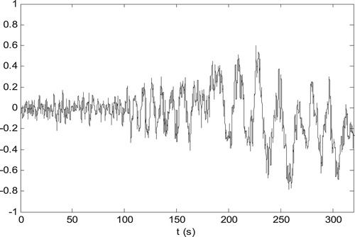
In the whole simulation process, collect the input–output measured data $\{u(t),y(t){\}}_{t=1,2\cdots 1000}$ within the closed-loop environment, and the number of data points which we can collect is equal to 2000. Apply this virtual reference feedback tuning control to design the controller parameters, the plant model $P(z)$ is excited by one sinusoidal input signal, whose curve is plotted in Figure 4 with the number of data points is 1000. In Figure 4, there are two curves, as one is the continue curve, the other is its discrete curve. The measured output response curve is plotted in Figure 5. The classical least squares algorithm is used to solve the optimization problem (14(14) $\begin{array}{rl}& \underset{\theta ,\eta }{min}{J}_{VR}^N(\theta ,\eta )\\ & =\frac{1}{N}\sum _{t=1}^N[u(t)-C_1(z,\theta )(M^{-1}(z)-C_2(z,\eta ))y(t){]}^2\\ & +\frac{1}{N}\sum _{t=1}^N{[u(t)+C_1(z,\theta )C_2(z,\eta )\frac{S(z)}{S(z)-1}y(t)]}^2\end{array}$(14) ). Before starting this recursive algorithm, the initial values of the unknown parameter vector are selected as. $\theta =\left[\begin{array}{c}0.7\\ 0.2\\ 0.1\end{array}\right],\eta =\left[\begin{array}{c}0.26\\ 0.1\\ 0.01\\ -0.01\\ -0.071\end{array}\right]$ Based on the input and output data $\{u(t),y(t){\}}_{t=1,2\cdots 1000}$, which are sampled in their own curves,respectively, we need to prove two aspects here, i.e. one is the identification algorithm, and the other is the statistical accuracy analysis or variance analysis with respect to the unknown controller parameters.

Figure 4. The input signal.

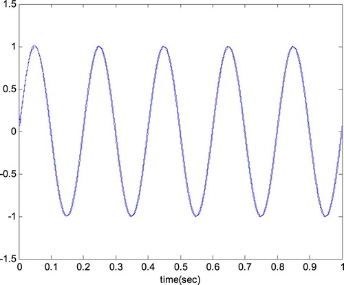
Figure 5. The measured output signal.

Firstly one experiment is given with the input signal in Figure 4, and the output signal in Figure 5, then the classical recursive least squares algorithm is applied to identify the unknown parameter vectors $(\theta ,\eta )$. After the parameter estimators $({\hat{\theta }}_N,{\hat{\eta }}_N)$ are obtained, how about the identification accuracy for these parameter estimators $({\hat{\theta }}_N,{\hat{\eta }}_N)$? To illustrate this aspect, we substitute the parameter vector ${\hat{\theta }}_N$ into the closed-loop transfer function from the excited signal $r(t)$ to the measured output $y(t)$ and compare this actual closed-loop transfer function with its expected or designed closed-loop transfer function $M(z)$. 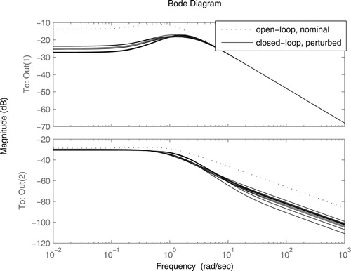Figure 6 shows the comparisons of the Bode responses between this actual closed-loop transfer function with its expected closed-loop transfer function $M(z)$. From Figure 6, we see these two closed loop transfer functions are very close, it means their approximation error can be neglected. 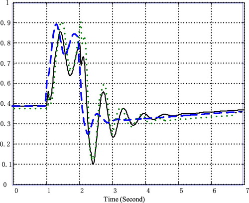Furthermore in Figure 6, the open-loop transfer function from $r(t)$ to $y(t)$ is given too, then the merit of the closed-loop system is easily seen.Secondly to illustrate the statistical accuracy analysis or variance analysis for the parameter estimators $({\hat{\theta }}_N,{\hat{\eta }}_N)$, for clarity of presentation, we only give the variance curves for the parameter estimator ${\hat{\theta }}_N$ in Figure 7, as only three elements exist in the parameter estimator ${\hat{\theta }}_N$. Observing these three variance curves with respect to the three unknown parameters $\{{\hat{\theta }}_1,{\hat{\theta }}_2,{\hat{\theta }}_3\}$, from the initialization to 1 s, three variance errors are almost same, then from 1 to 3 s, three variance errors will start to oscillate, and these generated derivation errors experience until to 3 s. From 3 s, three variance errors are stable and approach to one same constant value. Moreover form the variance analysis with respect to the three elements in the parameter vector θ, the classical least squares algorithm is not suited to identify the unknown controller parameters, as the parameter estimators identified by this algorithm are all biased. This identification result is not our expected goal, so other identification algorithms are needed to consider again, for example, our proposed identification algorithms from previous published papers (Jianhong, 2012, 2013, 2014a, 2014b, 2017, 2019). Generally statistical accuracy analysis can used to testify whether or not the identification accuracy is efficient or asymptotic efficient.

Figure 6. Comparisons of the Bode responses.

9. Conclusion

1. In this paper, from a statistical point of view, statistical accuracy analysis for virtual reference feedback tuning is studied for closed-loop system with two degrees of freedom controllers. When two desired closed-loop transfer functions are given, virtual input and virtual disturbance are constructed respectively to obtain one cost function, which corresponds to two model-matching problems. The classical least squares algorithm is applied to identify the unknown controller parameters on the condition of transforming that cost function as its simplified linear regression form. Then probability theory and matrix theory are introduced to derive the asymptotic variance matrix of the parameter vector, so that optimal input design and model structure validation can be analysed based on our obtained asymptotic variance matrix.

2. As this paper is our extended previous research on the basis of our many published papers, relating with virtual reference feedback tuning control, our goal in this paper is to give a complete analysis and summary for our previous work. Then our future work will turn to nonlinear and adaptive control.

Figure 7. Variance analysis for the first three parameters.

Acknowledgments

This work was supported by the Natural Science Foundation of China (Grant No. 60874037) and the Grants from the Foundation of Jiangxi University of Science and Technology (No. jxxjb18020). The first author is grateful to Professor Eduardo F Camacho for his warm invitation in his control lab at the University of Seville, Seville, Spain. Thanks for his assistance and advice on zonotopes in guaranteed state estimation and model predictive control.

Disclosure statement

No potential conflict of interest was reported by the authors.

Data availability statement

The data used to support the findings of this study are available from the corresponding author upon request.

Additional information

Funding

This work was supported by the Natural Science Foundation of China [grant number 60874037] and the Grants from the Foundation of Jiangxi University of Science and Technology [grant number jxxjb18020].

References

- Alamo, T., Bravo, J. M., & Camacho, E. F. (2005). Guaranteed state estimation by zonotopes. Automatica, 41(6), 1035–1043. https://doi.org/10.1016/j.automatica.2004.12.008
- Bazanella, A. S., Gevers, M., Mišković, L., & Anderson, B. D. O. (2008). Iterative minimization of H2 control performance criterion. Automatica, 44(10), 2549–2559. https://doi.org/10.1016/j.automatica.2008.03.014
- Bravo, J. M., Alamo, T., & Camacho, E. F. (2006). Bounded error identification of systems with time varying parameters. IEEE Transactions on Automatic Control, 51(7), 1144–1150. https://doi.org/10.1109/TAC.2006.878750
- Bravo, J. M., Alamo, T., Vasallo, M., & Gegundez, M. E. (2017). A general framework for predictors based on bounding techniques and local approximation. IEEE Transactions on Automatic Control, 62(7), 3430–3435. https://doi.org/10.1109/TAC.2016.2612538
- Bravo, J. M., Suarez, A., Vasallo, M., & Alamo, T. (2016). Slide window bounded error time varying systems identification. IEEE Transactions on Automatic Control, 61(8), 2282–2287. https://doi.org/10.1109/TAC.2015.2491539
- Campi, M. C., Lecchini, A., & Savaresi, S. M. (2002). Virtual reference feedback tuning: A direct method for the design of feedback controllers. Automatica, 38(8), 1337–1346. https://doi.org/10.1016/S0005-1098(02)00032-8
- Campi, M. C., Lecchini, A., & Savaresi, S. M. (2005). An application of the virtual reference feedback tuning method to a benchmark problem. European Journal of Control, 9(1), 66–76. https://doi.org/10.3166/ejc.9.66-76
- Campi, M. C., & Savaresi, S. M. (2006). Direct nonlinear control design: The virtual reference feedback tuning (VRFT) approach. IEEE Transactions on Automatic Control, 51(1), 14–27. https://doi.org/10.1109/TAC.2005.861689
- Campi, M. C., & Weyer, E. (2002). Finite sample properties of system identification methods. IEEE Transactions on Automatic Control, 47(8), 1329–1334. https://doi.org/10.1109/TAC.2002.800750
- Care, A., Csorji, B., Campi, M. C., & Weyer, E. (2018). Finite-sample system identification: An overview and a new correlation method. IEEE Control Systems Letters, 2(1), 61–66. https://doi.org/10.1109/LCSYS.2017.2720969
- Guardabassi, G. O., & Savaresi, S. M. (2012). Virtual reference direct design method: An off-line approach to data-based control system design. IEEE Transactions on Automatic Control, 45(5), 954–959. https://doi.org/10.1109/9.855559
- Jianhong, W. (2012). Virtual reference feedback tuning control for constrained closed loop system. Journal of Shanghai Jiaotong University, 46, 1398–1405. https://doi.org/1006-2467
- Jianhong, W. (2013). Virtual reference feedback tuning control design for nonlinear closed loop system. Electronic Optics and Control, 20, 23–27. https://doi.org/10.3969/j.issn.1671X.2013.01.006
- Jianhong, W. (2014a). Regularization design of virtual reference feedback tuning time varying control. Electronic Optics and Control, 21, 77–82. https://doi.org/10.3969/j.issn.1671-637X.2014.08.017
- Jianhong, W. (2014b). Virtual reference feedback tuning control and iterative minimization identification. Systems Engineering Theory and Practice, 34, 1256–1266. https://doi.org/1000-6788
- Jianhong, W. (2017). Virtual reference feedback tuning design in internal model control. Journal of System Science and Mathematical Science, 37, 355–369. https://doi.org/123.57.41.99/jweb_xtkxysx/CN/93C40
- Jianhong, W. (2019). Zonotope parameter identification for virtual reference feedback tuning control. International Journal of Systems Science, 50(2), 351–364. https://doi.org/10.1080/00207721.2018.1552767
- Lecchini, A., Campi, M. C., & Savaresi, S. M. (2002). Virtual reference feedback tuning for two degrees of freedom controllers. International Journal of Adaptive Control and Signal Processing, 16(5), 355–371. https://doi.org/10.1002/(ISSN)1099-1115
- Milanese, M., & Novara, C. (2004). Set membership identification of nonlinear systems. Automatica, 40(6), 957–975. https://doi.org/10.1016/j.automatica.2004.02.002
- Sala, A., & Esparza, A. (2005). Extension to virtual reference feedback tuning: A direct method for the design of feedback controllers. Automatica, 41(8), 1473–1476. https://doi.org/10.1016/j.automatica.2005.02.008
- Tanaskovic, M., Fagiano, L., Novara, C., & Morari, M. (2017). Data-driven control of nonlinear systems: An on-line direct approach. Automatica, 75, 1–10. https://doi.org/10.1016/j.automatica.2016.09.032
- Weyer, E. (2000). Finite sample properties of system identification of ARX models under mixing conditions. Automatica, 36(9), 1291–1299. https://doi.org/10.1016/S0005-1098(00)00039-X
- Weyer, E., Campi, M. C., & Csáji, B. C. (2017). Asymptotic properties of SPS confidence regions. Automatica, 82, 287–294. https://doi.org/10.1016/j.automatica.2017.04.041