A node three-dimensional localization algorithm based on RSSI and LSSVR parameters optimization

Abstract

To reduce the influence of received signal strength indication (RSSI) on ranging error, as well as the influence of least squares support vector regression (LSSVR) on localization algorithm, a node three-dimensional localization algorithm based on RSSI and LSSVR parameter optimization is proposed. First, the RSSI average values at 1–25m in four different directions are collected by experiments and the weighted recursive mean optimization method is used to optimize the values of RF factor and propagation factor. Then, the parameters of RBF kernel function and grid width of LSSVR are optimized. Finally, the RSSI range values are used as the input of LSSVR localization model, and the LSSVR regression model is used to solve, in this way, the location estimation of unknown WSN nodes is realized. The simulation results show that the average localization error of the algorithm without parameter optimization is 21.82%, and the localization error of the algorithm after parameter optimization is 11.70%, which has higher localization accuracy. At the same time, a node three dimensional localization experiment platform was built to verify the proposed algorithm in the actual environment, and the test results verified the effectiveness and superiority of the proposed algorithm.

KEYWORDS:

• Wireless sensor network
• received signal strength indication
• least squares support vector regression
• three-dimensional localization

1. Introduction

In wireless sensor network (WSN) applications, such as environment monitoring and target tracking, most sensor nodes are randomly deployed, and most of their locations are unknown (Langendoen & Reijers, 2013). In fact, only data with known spatial location information has practical value. Therefore, it is necessary to use localization technology to estimate the location of the sensor nodes. The node localization based on wireless sensor network means that a large number of sensor nodes deployed in the monitoring area to realize the estimation of the target location through information perception, cooperative signal and information processing (Han et al., 2020).

WSN localization algorithm can be divided into range-based localization and range-free localization according to whether the localization process needs ranging or not (Anup & Takuro, 2017). The former means that the distance between the unknown node and the anchor node needs to be estimated when estimating the location of the unknown node, that is, distance measurement. The latter uses the connectivity of the whole network to estimate the location of unknown nodes. Therefore, the accuracy of range-based algorithm is better than that of range-free algorithm. The ranging strategies commonly used in ranging and localization algorithms are angle of arrival (AOA), time of arrival (TOA), received signal strength index (RSSI). Among them, RSSI-based ranging uses the signal strength of the unknown node received from the anchor node to estimate the path propagation loss and then estimates the distance. Because RSSI-based ranging does not need additional hardware, it is widely used in low-cost WSN (Itoh et al., 2002). While the mapping relationship between RSSI value and distance value is a random process, and it is greatly affected by additive noise, model error, multipath propagation, non line of sight (NLOS) and other factors in actual measurement, which makes the accuracy of RSSI ranging method not high. Therefore, it is of great theoretical significance and practical value to study and seek a higher precision RSSI ranging algorithm.

Ranging-based WSN localization algorithm, such as trilateration method (Chen & Liu, 2016), weighted centroid algorithm (Cheng et al., 2019), maximum likelihood estimation method (Lu & Xia, 2016), least squares support vector regression (LSSVR) machine (Zhang et al., 2014), etc. LSSVR is a regression learning machine based on statistical learning theory. LSSVR uses equality constraints instead of inequality constraints to transform complex convex quadratic programming problems into simpler linear equations to solve. LSSVR regression is used to model the mapping relationship between eigenvectors and target coordinates, and a regression model that approximately reflects the mapping relationship between them is obtained. It has the characteristics of high calculation efficiency, good prediction ability, anti-noise performance, and good generalization ability in the case of small samples. We can map the measurement vectors based on the measurement information of the nodes, and then get the coordinate estimation of the target nodes. Appling LSSVR to WSN node localization, under the condition of limited hardware, can improve the effect of modelling and localization, reduce the error of node localization caused by noise and improve the accuracy of node localization (Zhang et al., 2014). Therefore, the WSN node localization algorithm based on RSSI and LSSVR has strong advantages. He and Huang (2013) proposed a LSSVR localization algorithm, which modelling parameters were optimized by PSO algorithm. Svečko et al. (2015) proposed a particle filter algorithm for distance estimation using multiple antennas on the receiver’s side and only one transmitter, where a received RSSI of radio frequency (RF) was used. Ding and Dong (2019) proposed a localization algorithm based on RSSI distance. As the distance was less than 10 m or not, the position can be calculated by the ‘Mini-Max Positioning Method’ or ‘Maximum Likelihood Estimation Method’, respectively. The above localization methods take RSSI method or LSSVR method, and optimize these methods. He et al. (2011) proposed a three-dimensional WSN nodes localization algorithm based on RSSI and LSSVR method. In this paper, RSSI or LSSVR had no improvement. Zhang et al. (2012) proposed a novel modelling parameters optimization method for target localization in WSN based on LSSVR by sampling measurement data. According to the method, RSSI of the target node respectively placed in sample locations were recorded by reference nodes to form a sampled RSSI dataset. Xia et al. (2019) first filtered out RSSI value with large deviation with Gaussian function, and then transformed into distance via these values, which would be served as the input of LSSVR model, and estimated the location of unknown nodes. In these papers, RSSI ranging and LSSVR localization methods are used, but only RSSI ranging method or LSSVR localization method is improved. Moreover, they also do not test the effectiveness of the proposed method.

Based on the advantages of RSSI ranging method and LSSVR localization method, a novel node three-dimensional localization algorithm based on RSSI and LSSVR is proposed. The proposed method takes the RSSI ranging values as the inputs of the LSSVR localization model, and three-dimensional localization of nodes are realized through the LSSVR regression modelling. Moreover, when processing the RSSI values, we put the RSSI values of continuous sampling into a queue with length of $n$ in turn. When a new RSSI value is collected, the first RSSI value in the queue will be removed to ensure that the length of the queue remains the same. When receiving the new RSSI value, the average RSSI value in the queue is calculated, which not only ensures the stability of RSSI value, but also ensures the sampling period of RSSI. In the process of LSSVR localization, the localization error is taken as the evaluation index, and the RBF kernel function parameter and the grid width parameter of LSSVR are optimized by experiment in real environment to improve the localization accuracy. On this basis, a corresponding WSN node three-dimensional localization experiment platform is developed, and the localization experiments are carried on to verify the proposed algorithm through that platform. The experimental results show that the localization method proposed in this paper has higher localization accuracy.

2. RSSI ranging model and parameter optimization

2.1. RSSI ranging model

The localization technology based on RSSI ranging has some advantages like as relatively small influence by NLOS, easy access to ranging data, and don’t need additional hardware for sensor nodes (Bianchi et al., 2019). In the process of wireless communication, there is a relationship between the signal power of the transmitting device and the signal power of the receiving device when transmitting data as shown in equation (1). Among them, $P_R$ is the signal power received by the receiving device, $P_T$ is the power transmitted by the transmitting device, $d$ is the distance between the transmitting device and receiving device, n is the propagation factor of the wireless signal, and the value of $n$ depends on the medium environment of the wireless signal propagation. (1) $\begin{array}{r}{P}_R=\frac{P_T}{d^n}\end{array}$(1)

Take logarithm on both sides of Equation (1) to get: (2) $\begin{array}{r}10n\lg d=10\lg \frac{P_T}{P_R}\end{array}$(2)

Since the transmitting power of the node is known, it can be obtained by bringing the transmitting power into Equation (2): (3) $\begin{array}{r}10\lg P_R=A-10n\lg d\end{array}$(3)

On the left side of Equation (3), $10\lg P_R$ is the expression for converting the wireless signal power received by the receiving device into the unit dBm. In this way, Equation (3) can be written as equation (4). (4) $\begin{array}{r}{P}_R(dBm)=A-\text{10}n\lg d\end{array}$(4)

In Equation (4), $A$ is the RF factor, whose value is usually the strength value of the wireless signal when the distance between the transmitting device and the receiving device is $1\text{m}$. It can be seen from Equation (4) that as long as the values of RF factor $A$ and propagation factor $n$ in the equation can be determined, the relationship between $P_R(dBm)$ (RSSI value) and distance $d$ can be determined, so that the distance between the transmitting device and the receiving device can be calculated according to the RSSI value. However, the values of $A$ and $n$ are usually empirical values, which are related to the specific sensor nodes and the medium environment of wireless signal transmission. To obtain accurate distance information through RSSI value, we design the corresponding actual environment experiment to realize the optimization of $A$ and $n$.

2.2. Optimization of RSSI ranging parameters

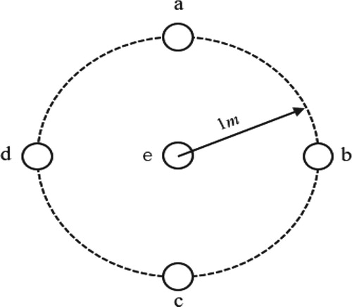
We calibrate the RF factor $A$ by experiment. Omnidirectional antenna is selected for the experimental test, and it is arranged according to the distribution of Figure 1. In Figure 1, T1,T2,T3, and T4 are transmitting devices and R is receiving device. To prevent channel conflict, the four transmitting devices T1,T2,T3, and T4 send 30 wireless packets to the receiving device R in turn. The receiving device extracts the RSSI values from the received wireless packets.

Figure 1. Layout of sensor nodes of RF factor $A$ calibration experiment.

According to the method described above, the original RSSI values at 1 m in four different directions (T1,T2,T3,T4) are all fluctuating, that is, the RSSI values collected at the same location are unstable. The instability of RSSI will directly lead to an increase of localization error. Therefore, we need to filter the original RSSI data. In this paper, recursive mean optimization method is used for optimization (Liu, 2018). The specific implementation process is as follows: put the RSSI values of continuous sampling into a queue with a length of 5, and the queue address numbers are 0, 1, 2, 3 and 4 from right to left. When a new RSSI value is collected, remove the RSSI value with address number 0, move the remaining four RSSI values to the left one bit in turn, and store the new RSSI value in the address number 4 of the queue to ensure that the length of the queue remains unchanged. After the new queue is formed, the average value of 5 RSSI values in the queue is calculated. This not only ensures the stability of RSSI value, but also ensures the sampling period of RSSI. Figure 2 is the RSSI values at 1 m in four different directions received by the receiving device.

Figure 2. RSSI values at 1 m in four different directions.

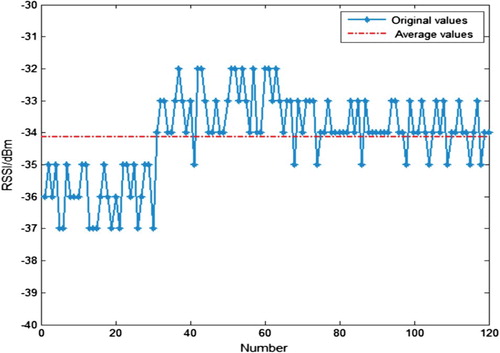
According to the order of T1,T2,T3, and T4, the number 1–30 are the values of RSSI at T1, the number 31–60 are the values of RSSI at T2, the number 61–90 are the values of RSSI at T3, and the number 91–120 are the values of RSSI at T4. As can be seen from Figure 2, since the antenna of the node is not an ideal omnidirectional antenna, the values in almost every direction are different. The red imaginary line is the average value of RSSI at 1 m in four directions. The value is −33.9, that is to say, the value of $A$ calibrated by experiment in the real environment is −33.9.

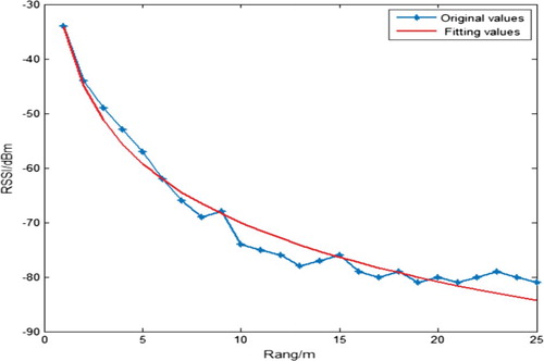
As can be seen from Figure 3, the RSSI value gradually decreases with the increase of the distance between nodes. The relationship between RSSI and distance in Figure 3 is fitted according to equation (4). The fitted curve is shown in the fitting data in Figure 3. The expression after fitting is: $\text{RSSI}(\text{dBm})=-(34.1+35.8\lg r)$. Therefore, we can determine the propagation factor value as 3.58. At the same time, it can be seen from Figure 3 that the RSSI value decays at a higher rate with the distance from 1 to 15 m. While from 15 to 25 m, the RSSI value decays slowly. Therefore, for localization technology based on the RSSI ranging, to ensure the accuracy of the unknown node localization, the distance between nodes should be within 15 m as much as possible during the network localization.

Figure 3. The relationship between distance and RSSI.

3. LSSVR-based localization algorithm and parameters optimization

3.1. Node three-dimensional localization algorithm based on LSSVR

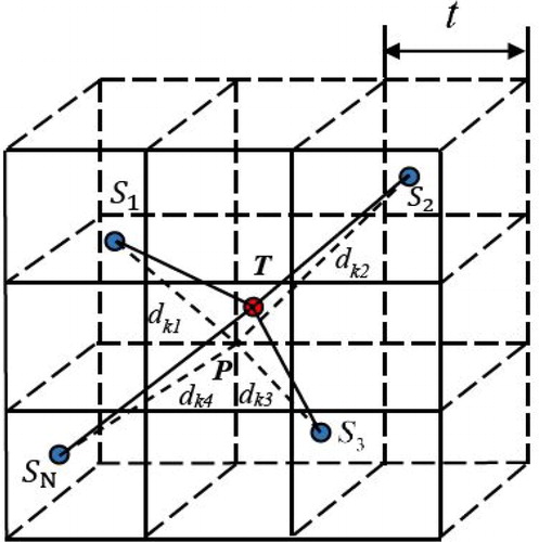
The detection object proposed in this paper, the three-dimensional localization scene Q, is a three-dimensional cube. It is transformed into a number of small cubes with length, width, and height are all $t$ using the grid width of size, as shown in Figure 4, where $S_i(i=1,2,\dots ,N)$ are the anchor nodes, and $T(x_i,y_j,z_j)$ is the unknown node. According to the basic principles of LSSVR and the node localization ideas of LSSVR, combining RSSI ranging method and LSSVR localization algorithm, the steps of node three-dimensional localization based on RSSI and LSSVR are as follows (Zhang, 2010):

1. Obtain training sample points: In the three-dimensional localization area $Q$, $t$ is the width of the three-dimensional grid divided by the three-dimensional localization area $Q$. Suppose the virtual nodes formed by the intersections of M grids are $P_k(x_k,y_k,z_k)(k=1,2,\dots ,M)$. Then the array $p_k$ is the sample points of the LSSVR localization algorithm training model.

2. Form a training sample set: Suppose that the distance from each element in array $P_k$ to anchor node $S_i$ is $d_{ki}$, then the distance vector from each element in array $P_k$ to anchor node $S_i$ is $v=(d_{k1}{d}_{k2},\dots ,d_{kN})$. Using a distance vector from any virtual node $P_k$ to each anchor node $S_i$ to construct a feature vector as $V_k=[v_{i1},v_{i2},\dots ,v_{iN}]$, a training sample set $U_x$, $U_y$, $U_z$ composed of the feature vector $V_k$ and elements $(x_k,y_k,z_k)$ of the array $P_k$ are shown in Equation (5). (5) $\begin{array}{r}\{\begin{array}{c}{U}_x=\{(V_k,x_k)|k=1,2,\dots ,M\}\\ U_y=\{(V_k,y_k)|k=1,2,\dots ,M\}\\ U_z=\{(V_k,z_k)|k=1,2,\dots ,M\}\end{array}\end{array}$(5)

3. Normalize training samples: normalize the input and output of training samples. For the training sample set $U_x$, the calculation method of the mean ${\mu }_i$ and standard deviation ${\sigma }_i$ of the $i$-th eigenvalue $v_{ik}(i=1,2,\dots ,N;k=1,2,\dots ,M)$ of the input vector is shown in Equations (6) and (7). (6) $\begin{array}{rl}{\mu }_i& =\frac{1}{M}\sum _{k=1}^M{v}_{ik}\end{array}$(6) (7) $\begin{array}{rl}{\sigma }_i& =\sqrt{\frac{1}{M-1}\sum _{k=1}^M{(v_{ik}-{\mu }_i)}^2}\end{array}$(7)

Figure 4. The localization principles of LSSVR in three-dimensional coordinate system.

The normalized eigenvalue $v{{}^{\mathrm{\prime }}}_{ik}$ is obtained as shown in Equation (8). (8) $\begin{array}{r}v{}_{ik}^{\mathrm{\prime }}=\frac{v_{ik}-{\mu }_i}{{\sigma }_i}\end{array}$(8)

Calculate the mean ${\mu }_x$ and standard deviation ${\sigma }_x$ of the output $x$ coordinate $x_k(k=1,2,\dots ,M)$ according to Equations (9) and (10). (9) $\begin{array}{rl}{\mu }_x& =\frac{1}{M}\sum _{k=1}^M{x}_k\end{array}$(9) (10) $\begin{array}{rl}{\sigma }_x& =\sqrt{\frac{1}{M}\sum _M^1{(x_k-{\mu }_x)}^2}\end{array}$(10)

Then the normalized output $x$ coordinate is shown in Equation (11). (11) $\begin{array}{r}{x_k}^{\mathrm{\prime }}=\frac{x_k-{\mu }_x}{{\sigma }_x}\end{array}$(11)

Similarly, the normalized output $y$ coordinate and $z$ coordinate can be obtained, as shown in Equations (12) and (13). (12) $\begin{array}{rl}{y_k}^{\mathrm{\prime }}& =\frac{y_k-{\mu }_y}{{\sigma }_y}\end{array}$(12) (13) $\begin{array}{rl}{z_k}^{\mathrm{\prime }}& =\frac{z_k-{\mu }_z}{{\sigma }_z}\end{array}$(13)

(4)

Train localization model: Use the LSSVR localization model to train the sample sets $U_x$, $U_y$, $U_z$, respectively. Construct and solve the optimization problem shown in Equation (14) for $U_x$. (14) $\begin{array}{r}\{\begin{array}{c}\underset{\omega ,\xi ,b}{min}\frac{1}{2}{\omega }^2+\gamma \frac{1}{2}\sum _{i=1}^M{{\xi }_i}^2\\ s.t.\begin{array}{c}\end{array}{x}_k={\omega }^T\varphi (V_k)+b+{\xi }_k,k=1,2,\dots ,M\end{array}\end{array}$(14) where $\varphi ()$ is a nonlinear mapping function, $b$ is a deviation, $\omega$ is a weight, $\gamma$ is a regularized parameter, and ${\xi }_i$ is a random error. The nonlinear mapping function selected in this paper is the RBF kernel function, as shown in Equation (15). (15) $\begin{array}{r}R(V_m,V_n)=exp(\frac{-V_m,{V_n}^2}{2{\sigma }^2})(m,n=1,2,\dots ,M)\end{array}$(15) where ${\sigma }^2$ is the kernel function parameter. The above problem is transformed into solving Lagrange operators $a$ and $b$ in Equation (16). (16) $\begin{array}{r}\{\begin{array}{c}\left[\begin{array}{cc}0& {\overline{1}}^T\\ \overline{1}& \mathrm{\Omega }+{\gamma }^{-1}I\end{array}\right]\left[\begin{array}{c}b\\ a\end{array}\right]=\left[\begin{array}{c}0\\ x^{\mathrm{\prime }}\end{array}\right]\\ \left[\begin{array}{cc}0& {\overline{1}}^T\\ \overline{1}& \mathrm{\Omega }+{\gamma }^{-1}I\end{array}\right]\left[\begin{array}{c}b\\ a\end{array}\right]=\left[\begin{array}{c}0\\ y^{\mathrm{\prime }}\end{array}\right]\\ \left[\begin{array}{cc}0& {\overline{1}}^T\\ \overline{1}& \mathrm{\Omega }+{\gamma }^{-1}I\end{array}\right]\left[\begin{array}{c}b\\ a\end{array}\right]=\left[\begin{array}{c}0\\ z^{\mathrm{\prime }}\end{array}\right]\end{array}\end{array}$(16) where $x^{\mathrm{\prime }}=[x_1^{\mathrm{\prime }},x_2^{\mathrm{\prime }},\dots ,x_M^{\mathrm{\prime }}{]}^T$, $x^{\mathrm{\prime }}=[y_1^{\mathrm{\prime }},y_2^{\mathrm{\prime }},\dots ,y_M^{\mathrm{\prime }}{]}^T$, $x^{\mathrm{\prime }}=[z_1^{\mathrm{\prime }},z_2^{\mathrm{\prime }},\dots ,z_M^{\mathrm{\prime }}{]}^T$, $a=[a_1,a_2,\dots ,a_M{]}^T$, $\overline{1}=[1,1,\dots ,1{]}^T$, $\mathrm{\Omega }(m,n)=R(V_m,V_n)$.

From $\left[\begin{array}{c}b\\ a\end{array}\right]=\left[\begin{array}{cc}0& {\overline{1}}^T\\ \overline{1}& \mathrm{\Omega }+{\gamma }^{-1}I\end{array}\right]\left[\begin{array}{c}o\\ x^{\mathrm{\prime }}\end{array}\right]$, $a$ and $b$ can be derived, so as to obtain the decision function shown in Equation (17). (17) $\begin{array}{r}\hat{x}=f_x(V)=\sum _{k=1}^M{a}_{k}R(v,V_k)+b\end{array}$(17)

This is the localization model X-LSSVR with output coordinate $x$. Similarly, the localization models Y-LSSVR with output coordinate $y$ and Z-LSSVR with output coordinate $z$ can be obtained.

(5)

RSSI ranging of unknown nodes: The distance $d_i(i=1,2,\dots ,N)$ from unknown nodes $T(x_i,y_j,z_j)$ to $S_i(i=1,2,\dots ,N)$ is measured using the RSSI ranging method with the optimized parameters mentioned above, and distance vector $w=(d_1,d_2,\dots ,d_N)$ from unknown nodes to anchor nodes is obtained.

(6)

Calculate coordinate: The distance vector $w$ obtained in step (4) is used as the input vector of the node three-dimensional localization model X-LSSVR, Y-LSSVR and Z-LSSVR. The LSSVR localization model is used for modelling, and the output of the decision function is denormalized to obtain the estimated coordinates of the unknown node as shown in Equation (18). (18) $\begin{array}{r}\{\begin{array}{c}\hat{x}=f_x(V)\bullet {\sigma }_x+{\mu }_x\\ \hat{y}=f_y(V)\bullet {\sigma }_y+{\mu }_y\\ \hat{z}=f_z(V)\bullet {\sigma }_z+{\mu }_z\end{array}\end{array}$(18)

3.2. Optimization of LSSVR parameters

3.2.1. Optimization of grid width for LSSVR localization algorithm

It can be seen from the LSSVR node three-dimensional localization algorithm that the size of the grid width $t$ in the LSSVR localization algorithm directly affects the size of the training sample, which in turn affects the accuracy and real-time performance of the localization. On the one hand, the spatial distribution area of the training sample is the modelling area of LSSVR regression modelling. The density of the samples directly determines the generalization ability of the LSSVR model. The denser the sample is, the better the generalization ability will be, and the higher the localization accuracy will be. On the other hand, with the increase of the number of the training sample, it will increase the calculation of LSSVR modelling localization, thus affecting the real-time localization. Therefore, we need to select a suitable training sample area, that is, the size of the grid width parameter t, and meet the requirements of localization accuracy and real-time.

The grid width $t$ in LSSVR localization algorithm directly affects the size of training samples, and then affects the real-time and accuracy of regression modelling localization. According to the relationship between RSSI and distance in Figure 3, when distance is in the range of 15 m, the change of RSSI value with distance is relatively obvious. Considering that in the experiment, the packet loss rate of RSSI at about 15 m is relatively high, while the packet loss rate of RSSI at about 10 m is very small. Considering the real environment and site constraints, the experimental area selected is 10 m*10 m*10 m. At the same time, we found it is meaningless when the grid width t is too large or too small. According to the preliminary experimental results, the range of grid width t is chosen as 1∼3.5 m. Set the ranging error as 0 in distance calculation. The simulation process of the optimization of grid width t is as follows:

1. First, set the positions of four anchor nodes, and set the corresponding coordinates as (0, 0, 0), (10, 0, 0) (0, 10, 0), (0, 0, 10).

2. In the range of grid width t=1∼3.5, the localization errors of 100 randomly assigned unknown nodes are calculated in step size of 0.5 m.

3. The average localization error curve of 100 nodes with different grid width is drawn.

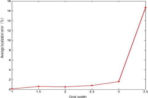
Figure 5 shows the average localization error curve of 100 nodes under different grid width. According to Figure 5, the average localization error of 100 unknown nodes increases with the increase of grid width. When the grid width t is 1∼2.5 m, the average localization error of 100 unknown nodes increases slowly. When the grid width t is 2.5 m, the average localization error is 0.8595%, less than 1%. When the grid width t is 3 m, the average localization error is 1.539%. When the grid width t is 3∼3.5 m, the average localization error increases sharply, more than 16%.

Figure 5. Average localization error of nodes with different grid width.

It is also found that the speed of LSSVR regression modelling has a big difference with the change of the grid width $t$ in the experiment. In this study, we set the localization frequency as 1s/time. To verify whether the localization frequency meets the requirements, it is necessary to verify the grid width $t$. Considering that when the grid width t is 3∼3.5 m, the average localization error is already large, and the grid width value in this range has no value. In this experiment, the grid width $t$ is set as 1∼3 m, and the step size is still 0.5 m. Figure 6 shows the localization time of a single node under different grid widths.

Figure 6. Localization time of a single node under different grid widths.

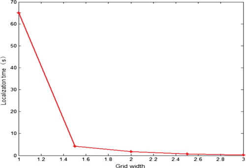
It can be seen from Figure 6 that with the increase of grid width t, the localization time of a single node gradually decreases. When $t$ =1.5 m, the localization time of single node is 4.221s; when $t$ =2 m, the localization time of single node is 1.733s; when $t$ =2.5 m, the localization time of single node is 0.688s; when $t$ =3 m, the localization time of single node is 0.285. Therefore, considering the balance of localization error and localization time, the grid width should be 2.5 m.

3.2.2. Optimization of LSSVR kernel function parameter

According to the previous description, we know that LSSVR localization algorithm is greatly affected by its parameters, and it needs to be optimized to improve the localization effect. In this paper, RBF function is chosen as the regression modelling function of LSSVR. The parameters that affect the regression modelling of LSSVR are kernel function parameter ${\sigma }^2$ and regularized parameter $\gamma$ (Zhang et al., 2010), Among them, the kernel parameter ${\sigma }^2$ directly affects the performance of LSSVR localization model, and the regular parameter γ can make a compromise between training error and localization model. The regularization parameter $\gamma$ is obtained by optimization of PSO algorithm, which is selected as 100 in this paper (Tong, 2018). In this experiment, the bisection method is used to determine the initial value range of the kernel function parameter ${\sigma }^2$. After many experiments, obtained the initial value range of ${\sigma }^2$ should be 1∼10. As in the previous experimental simulation environment, the experimental area is still 10 m*10 m*10 m, and the grid width t is preset as 2.5. 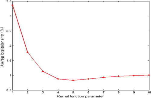The experimental procedure of the optimization of ${\sigma }^2$ is the same as that of the optimization of t. Through the simulation experiment, the node average localization error corresponding to different kernel function parameter ${\sigma }^2$ is obtained, as shown in Figure 7. With the increase of kernel function parameter ${\sigma }^2$, the average localization error decreases rapidly at first, and then increases slowly. The average localization error of 100 unknown nodes is the smallest when ${\sigma }^2$=5, its value is 0.7303%, lower than 1%, meets the expected value of the experiment. Therefore, in the proposed LSSVR localization algorithm, the RBF kernel function parameter ${\sigma }^2$ is optimized to be 5.

Figure 7. Average localization error of unknown node with different values of ${\sigma }^2$_.

4. Simulation and experimental analysis

4.1. Simulation experiment and result analysis

4.1.1. Simulation experiment with unoptimized parameters and result analysis

After the parameter optimization experiment, the kernel function parameters and grid width of LSSVR algorithm for WSN node three-dimensional localization are determined. To verify the feasibility and localization accuracy of the algorithm with the parameters, the algorithm with the unoptimized parameters and the optimal parameters are compared by experimental method. The above algorithm is simulated in MATLAB R2017b. The simulation environment is the same as the simulation environment of the previous optimization experiment. In the localization space, 100 unknown nodes are randomly spread for localization. The radio signal carrier frequency is 2.4 GHz, the communication radius is 10 m, and the preset average ranging error is e=10% (Tomic et al., 2017). The parameters are unoptimized, RBF kernel function parameter ${\sigma }^2$=2, grid width $t$ =4. The localization results of 100 unknown nodes are shown in Figure 8, and the corresponding localization errors are shown in Figure 9.

Figure 8. Localization results with the unoptimized parameters.

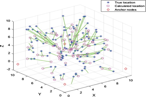
Figure 9. Localization errors with the unoptimized parameters.

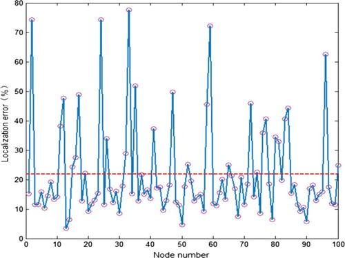
It can be seen from Figures 8 and 9 that localization of 100 unknown nodes in simulation environment with the unoptimized parameters, the localization error range is 3.422%∼77.67%, the average localization errors of 100 unknown nodes is 21.82%, the localization accuracy is not high, and the localization effect is poor.

4.1.2. Simulation experiment with optimized parameters and result analysis

In the environment with optimized parameters, the parameters selected are: RBF kernel parameter ${\sigma }^2=5$, grid width $t=2.5$, and the other simulation parameters remain unchanged. The localization result and localization errors of 100 unknown nodes are shown in Figures 10 and 11, respectively.

Figure 10. Localization results with the optimized parameters.

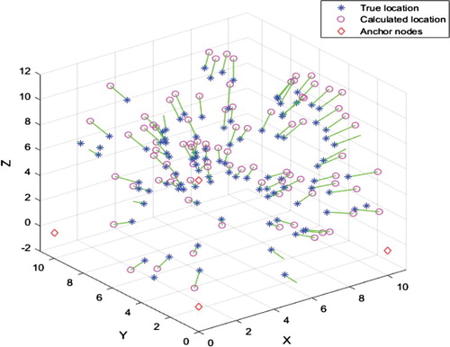
Figure 11. Localization errors with the optimized parameters.

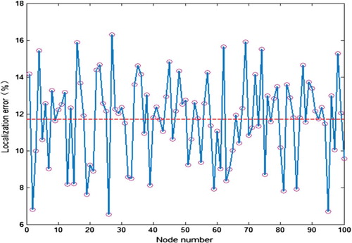
It can be seen from Figures 10 and 11 that in this simulation environment, the localization error range of 100 randomly distributed unknown nodes is 6.546%∼16.30%, and the average localization error is 11.70%. Compared with the localization errors in the experiment with unoptimized parameters, it reduces about 10% and has better localization effect.

4.2. Experiment in real environment and result analysis

4.2.1. Experimental environment and parameter setting

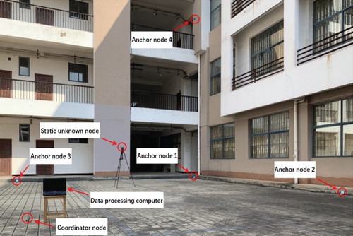
To verify the effectiveness and superiority of the localization method proposed, the corresponding experimental platform are set up for experimental testing. The hardware composition is as follows: (1) A computer installed with localization system software developed by us in Visual Studio using C# language, the processor of the computer is Inter Core(TM) i5-2450M CPU 2.5 GHz, the operating system is 64 bit windows10, and Matlab r2017b is installed on the computer. (2) Six CC2530 wireless sensor modules produced by TI company are networked using Z-Stack-CC2530-2.5.1a protocol stack. (3) A tripod with adjustable height, adjustable range: 0.5m∼2 m. The node three-dimensional localization experiment selects the open outdoor environment of larger than 10 m*10 m*10 m, as shown in Figure 12.

Figure 12. Environment of WSN node three-dimensional localization experiment.

4.2.2. Experimental procedure and result analysis

The experimental steps of WSN node localization are as follows: (1) Download the compiled programme to each node according to the node category. (2) Place the four anchor nodes in the coordinates (0, 0, 0), (10, 0, 0), (0, 10, 0), (0, 0, 10), and the coordinate unit is meter. (3) The unknown nodes are randomly deployed in the actual three-dimensional WSN environment in five times, and obtain their real coordinates (2, 2, 2), (3, 7, 0.5), (5, 5, 1), (7, 3, 1.5), (8, 8, 2) by measurement, respectively, and record the coordinate values. (4) Turn on the power of coordinator node, unknown node, and anchor node, the WSN network will organize by itself. (5) Open the localization system software, set the corresponding parameters, receive the data through the serial port to locate the three-dimensional unknown node, and obtain the location coordinates of the unknown node five times in turn.

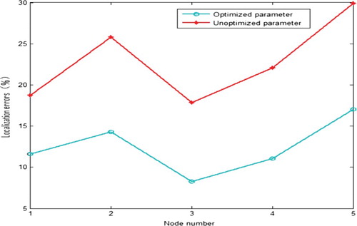
According to the above experimental steps, we can get the corresponding localization results. Figure 13 is a three-dimensional rendering of one-time localization results with the optimized parameters. Figure 14 shows the localization errors in the case of using unoptimized parameters and using optimized parameters. It can be seen from Figure 14 that when using the unoptimized parameters, in the node three-dimensional localization of WSN, the minimum localization error is 17.83%, the maximum localization error is 29.92% and the average localization error is 22.87%. While when using the optimized parameters, the minimum localization error is 8.27%, the maximum localization error is 17.03%, and the average localization error is 12.45%. Obviously, the localization effect under the condition of using optimized parameters is better than that the condition of using the unoptimized parameters, and the localization error is greatly reduced. At the same time, the results of simulation experiment and test experiment show that the localization error of actual test experiment is larger than that of simulation experiment. There are two main reasons for the difference between the two localization errors. One is that the data packets between nodes in WSN contain noise, which leads to noise errors. Besides, the RSSI value of CC2530 is converted to the distance value by the fitting equation, which will lead to the fitting error. Another is that the LSSVR modelling algorithm is used in this localization system. When there are infinite training samples, LSSVR regression model can accurately describe the mapping relationship between the feature vector and the target coordinate, and get the accurate target coordinate value. While in the actual modelling process, the number of training samples is limited, which leads to a certain model error in the target coordinate value. The existence of ranging error and algorithm model error makes the actual localization effect worse than the simulation localization effect.

Figure 13. Localization results of using the optimized parameters.

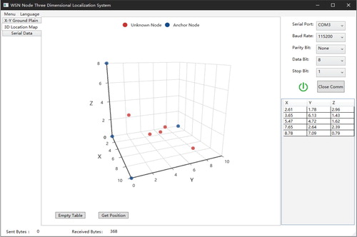
Figure 14. Localization errors of five unknown nodes.

5. Conclusion

In traditional RSSI ranging methods, the RF factor and the propagation factor are generally selected according to experience, which are not targeted and do not meet the needs of actual ranging. In this paper, the principle of RSSI ranging is analysed, and the optimization experiments of the corresponding RF factor and propagation factor are designed. LSSVR's good noise immunity can reduce the impact of RSSI fluctuations on localization results and improve localization accuracy. In this paper, the corresponding simulation experiments are designed to optimize the kernel function parameters and grid width of LSSVR localization model. Finally, the simulation experiment of MATLAB and the actual environment experiment are carried out to verify. The experimental results show that compared with using the unoptimized parameters, the average localization errors of LSSVR three-dimensional nodes using the optimized parameters are 10.14% and 5.84% less, respectively. Through theoretical research, simulation analysis and experimental verification, the following conclusions are reached:

1. Combining the advantages of RSSI ranging method and LSSVR localization method, a WSN node three-dimensional localization algorithm with RSSI and LSSVR parameters optimization is proposed. Compared with some existing algorithms, we have not only optimized the RF factor and propagation factor of the RSSI ranging model, but also the kernel function parameters and grid width of the LSSVR localization model, and we have designed corresponding experiments to optimize the parameters.

2. Based on the CC2530 wireless sensor module, we developed a WSN node three-dimensional localization experiment platform, and tested the proposed RSSI and LSSVR parameters optimized WSN node three-dimensional localization algorithm. The test results show that the localization effect of the proposed localization algorithm with optimized parameters is better than that of localization algorithm with the unoptimized parameters. At the same time, it is verified that the WSN node three-dimensional localization system developed by us can meet the requirements of actual localization experiments, and has certain engineering practical value.

3. Although the effectiveness of the proposed algorithm is verified through simulation experiment and actual environment experiment, both simulation experiment and actual environment experiment optimize RSSI ranging parameters and LSSVR localization parameters for a single parameter. How to establish a suitable objective function to achieve multi-parameter optimization to improve the localization effect is a content we will continue to study in further. Besides, in actual WSN applications, unknown nodes are generally mobile. The node three-dimensional localization is only studied under static conditions. How to apply the related methods to the three-dimensional localization of mobile nodes is another content we will study in the future.

Disclosure statement

No potential conflict of interest was reported by the author(s).

Correction Statement

This article has been republished with minor changes. These changes do not impact the academic content of the article.

Additional information

Funding

This work was supported by National Natural Science Foundation of China [No. 61741303], Guangxi Natural Science Foundation [NO. 2017GXNSFAA198161], the key laboratory of spatial information and geomatics (Guilin University of Technology) [No.15-140-07-23, No.16-380-25-23]. Innovation Project of Guangxi Graduate Education [No. YCSW2019159].

References

- Anup, K. P., & Takuro, S. (2017). Localization in wireless sensor networks: A survey on algorithms, measurement techniques, applications and challenges. Journal of Sensor and Actuator Networks, 6(4), 24. https://doi.org/10.3390/jsan6040024
- Bianchi, V., Ciampolini, P., & Munari, I. D. (2019). RSSI-based indoor localization and identification for ZigBee wireless sensor networks in smart homes. IEEE Transactions on Instrumentation and Measurement, 68(2), 566–575. https://doi.org/10.1109/TIM.2018.2851675
- Chen, L., & Liu, W. (2016). Ranging optimization based on RSSI and trilateration method. Journal of Hubei University of Technology, 31(2), 49–52. https://doi.org/10.3969/j.issn.1003-4684.2016.02.014
- Cheng, C., Jiang, Z. Y., Han, Q. S., & Wang, H. Z. (2019). Improved RSSI weighted centroid localization algorithm based on adaptive reference value. Journal of Jilin University (Science Edition), 57(2), 352–356. https://doi.org/10.13413/j.cnki.jdxblxb.2017440
- Ding, X. H., & Dong, S. (2019). Improving positioning algorithm based on RSSI. Wireless Personal Communications, 2019, 1–15. https://doi.org/10.1007/s11277-019-06821-0
- Han, D. Z., Yu, Y. P., Li, K. C., & Mello, R. F. (2020). Enhancing the sensor node localization algorithm based on improved DV-hop and DE algorithms in wireless sensor Networks. Sensors, 20(2), 343. https://doi.org/10.3390/s20020343
- He, X. W., & Huang, W. Q. (2013). Study on LSSVR modeling positioning based on particle swarm optimization. In B. Li & H. M. Zhang (Eds.), Advanced materials research (Vol. 791, pp. 1096–1099). Trans Tech Publications Ltd.
- He, X. W., Xiao, Y., & Wang, Y. (2011). A LSSVR three-dimensional WSN nodes location algorithm based on RSSI. In 2011 International Conference on Electrical and Control Engineering (pp. 1889–1895). IEEE.
- Itoh, K. I., Watanabe, S., Shih, J. S., & Sato, T. (2002). Performance of handoff algorithm based on distance and RSSI measurements. IEEE Transactions on Vehicular Technology, 51(6), 1460–1468. https://doi.org/10.1109/TVT.2002.804866
- Langendoen, K., & Reijers, N. (2013). Distributed localization in wireless sensor networks: A quantitative comparison. Computer Networks, 43(4), 499–518. https://doi.org/10.1016/S1389-1286(03)00356-6
- Liu, F. (2018). Single step recursive algorithm of permutation combination in deviation simulation. Missiles and Space Vehicles, 2018(5), 45–50. https://doi.org/10.7654/j.issn.1004-7182.20180510
- Lu, X. L., & Xia, W. R. (2016). Weighted centroid localization algorithm based on maximum likelihood estimation. Information and Control, 45(5), 582–587. https://doi.org/10.13976/j.cnki.xk.2016.0582
- Svečko, J., Malajner, M., & Gleich, D. (2015). Distance estimation using RSSI and particle filter. ISA Transactions, 55, 275–285. https://doi.org/10.1016/j.isatra.2014.10.003
- Tomic, S., Beko, M., & Dinis, R. (2017). 3-D target localization in wireless sensor networks using RSS and AoA measurements. IEEE Transactions on Vehicular Technology, 66(4), 3197–3210. https://doi.org/10.1109/TVT.2016.2589923
- Tong, Y. T. (2018). Study of least squares support vector regression. Zhejiang Normal University.
- Xia, M., Zhang, X., & Zhu, Y. (2019). Real time localization algorithm based on local linear embedding optimization in sensor networks. Cluster Computing, 22(2), 4173–4178. https://doi.org/10.1007/s10586-018-1697-y
- Zhang, X. P. (2010). Study on theory and algorithm of mobile target localization in WSN based on LSSVR regression modeling. South China University of Technology.
- Zhang, L. P., Ji, W. J., & Chen, M. (2014). Three-dimensional WSN node localization method based on LSSVR optimized by DE algorithm. Recent Advances in Electrical & Electronic Engineering, 7(2), 123–129. https://doi.org/10.2174/2213111607666140701174742
- Zhang, X. P., Liu, G. X., & Zhou, S. B. (2010). Target localization based on LSSVR in wireless sensor networks. Optics and Precision Engineering, 18(9), 2060–2068. https://doi.org/10.3788/OPE.20101809.2060
- Zhang, X. P., Wang, Y., & Liu, G. X. (2012). Modeling parameters optimization for target localization in WSN based on LSSVR by sampling measurement data. International Journal of Advancements in Computing Technology, 4(6), 346–357. https://doi.org/10.4156/ijact.vol4.issue6.40