A self-Adaptive CNN with PSO for bearing fault diagnosis

Abstract

Convolutional neural network (CNN) is now widely applied in bearing fault diagnosis, but the design of network structure or parameter tuning is time-consuming. To solve this problem, a particle swarm optimization (PSO) algorithm is used to optimize the network structure and a self-adaptive CNN is proposed in this paper. In the proposed method, a theoretical method is used to automatically determine the window size of short-time Fourier transform (STFT). To reduce the computation time, PSO is only applied to obtain the optimal key parameters in CNN with a small number of training samples and a small epoch number. To simplify the CNN structure, a fitness function considering the numbers of kernels and neuron nodes is used in PSO. According to the verification experiments for two well-known public datasets, the proposed method can get higher accuracy than other state-of-art methods. Furthermore, the parameters that are required to be input only involve the bearing parameters, so the proposed method can be applied in industry readily.

KEYWORDS:

• Bearing fault diagnosis
• deep learning
• adaptive CNN

1. Introduction

Rolling element bearings have been widely applied and are the most critical components in industrial machinery. According to our literature review, 40–55% of broken machines are caused by bearing faults (Boudinar et al., 2016; Hamadache et al., 2015; Harmouche et al., 2015; Rai & Upadhyay, 2016; Sohaib et al., 2017). The degradation of bearings can result in unexpected failures of machines, which lead to long downtimes, large economic losses, and serious human injuries. Therefore, the bearing fault diagnosis is regarded as an important tool for identification, prediction, and prevention of failures in rotating machinery.

Fault diagnosis techniques can be generally categorized into model-based, signal-based, knowledge-based, and hybrid fault diagnosis (Gao et al., 2015).

In signal-based methods, there are many kinds of signals such as vibration and acoustic signals (Liu et al., 2016), electric current (Boudinar et al., 2016), temperature (Yuan et al., 2018), and wear debris. Among these, the vibration signal is the most widely used approach (Lin & Ye, 2019; Sohaib et al., 2017). The signal processing methods generally include Fourier Transform (FT), Short-Time Fourier Transform (STFT), Wavelet Transform (WT), Wavelet Package Transform (WPT), Empirical Wavelet Transform (EWT), Hilbert-Huang Transform (HHT), Empirical Mode Decomposition (EMD), Variation Mode Decomposition (VMD), and Ensemble Empirical Mode Decomposition (EEMD). For more details on the advantages and disadvantages of these methods can be seen in Refs (Lin & Ye, 2019; Ma et al., 2018; Yi et al., 2016).

Nowadays, a signal-based method is always integrated with a knowledge-based method, which can be used to optimize the parameters in the signal-based method. For example, the particle swarm optimization (PSO) and quasi-Newton minimization algorithms are applied to seek optimal parameters of continuous wavelet transform models based on impulse modelling (Huo et al., 2017). Similarly, PSO is applied for the parameter optimization of VMD (Wang et al., 2018; Yi et al., 2016; Yuwono et al., 2016). On the other hand, the signal-based method can be used for handcrafted feature design and feature extraction, and then the knowledge-based method further makes use of these features to learn fault modes through training with historical data. Here, two kinds of methods, i.e. shallow machine learning and deep learning, are used for knowledge learning.

For the shallow machine learning methods, after the right set of features are designed, these features are fed into some shallow machine learning algorithms. For example, in references EMD-SVM (Zhang, Liang et al. 2015), HHT-SVM (Soualhi et al., 2015), DWT-KNN (Jung & Koh, 2015), WPT-KNN (Wang, 2016), WT-Naive Bayes (NB) (Seshadrinath et al., 2014), HHT-FFT-PCA (Harmouche et al., 2015), and EMD-PSO-SVM (Chen, Tang et al. 2014), signal processing methods including EMD, HHT, DWT, WPT, etc are used to extract features and SVM, KNN,NB,PCA are to perform classifications. PSO is used to determine the optimal parameters of SVM (Chen, Tang et al. 2014).

In the deep learning methods, Ref (Peng et al., 2017) use convolutional neural network (CNN) to diagnose fused signals of two sensors, where FFT is as are preprocessing method. Wavelet scalogram images are fed into CNN to detect faults (Wang et al., 2016). Similarly, three time–frequency analysis methods STFT, WT, and HHT are used to generate image representations of the raw signals which are fed into CNN (Verstraete et al., 2017). Adaptive overlapping CNN (AOCNN) with a sparse filter is proposed to deal with one-dimensional raw vibration signals directly. The adaptive convolutional layer and the root-mean-square (RMS) pooling layer are proposed to dealt with the shift variant problem (Qian et al., 2018). Time-domain and frequency-domain features are extracted from different sensor signals and then fed into multiple two-layer sparse auto encoder (SAE) for feature fusion, which is used to train deep belief network (DBN) for further classification (Chen & Li, 2017). A stacked sparse auto encoder is applied to automatically extract the fault features of sound spectrograms with STFT, and softmax regression is adopted as the method of classifying the fault modes (Liu et al., 2016). In Ref. (Jia et al., 2016), DNN based on a stack auto encoder is applied for roller bearing and planetary gearbox fault diagnosis using frequency spectra. In Ref. (Jiang et al., 2018), deep recurrent neural network (DRNN) is used to extract the features from the input spectrum sequences. In Ref. (Lei et al., 2016), the features are learnt through sparse filtering in an unsupervised way and then fed to softmax regression for classifying health conditions in a supervised manner (Lei et al., 2016).

In these two kinds of knowledge-based methods, deep learning can auto extract highly representative features while shallow machine learning methods require labour-intensive feature engineering, so it is widely researched all over the world. However, the design of network or parameter tuning is one time-consuming procedure, which affects the performance of the neuron network. For example, lots of existing CNN networks have been designed and applied, and different CNNs (Hoang & Kang, 2019; Verstraete et al., 2017; Wang et al., 2016; Wen et al., 2018) consisting of different convolution, pooling, and dense layers are proposed, which result in different performances. On account of this, most current research focuses on the development of the network. In order to design the optimized deep belief network, PSO is used for deciding the optimal network structure, including the optimal number of neurons in each hidden layer, the learning rate, and the momentum (Shao et al., 2015). Similarly, the main parameters of the deep CNN model are also determined with the PSO method (Fuan et al., 2017). In our method, a two-step training idea is introduced, which is different from that in Ref. (Fuan et al., 2017). The first-step is the optimization of the CNN structure, where the fitness function accounts the number of neuron nodes and trains the CNN parameters with a small number of training samples and a small epoch number. The second-step is the final training with the optimized CNN.

Through above literature review, it is obvious that the design of network or tuning parameters is a complex and time-consuming work. To relieve the burden, a Self-Adaptive CNN (SA-CNN) is proposed in this study. Because the PSO has the characteristics of fast convergence speed, small setting parameters and convenient implementation, it is used to optimize the key parameters in CNN (Yuwono et al., 2016).

Although CNN can auto extract features, to accelerate the evolution of PSO, signal processing is taken as a preprocessing method to extract basic time–frequency information. Among signal processing methods reviewed before, WT analysis is restricted by mutually selected wavelet basis function and the number of decomposition levels (Wang et al., 2018); Empirical wavelet transform (EWT) is restricted on choosing the boundaries of Fourier spectrum appropriately (Yi et al., 2016);HHT and EMD exists deficiencies such as model mixing and the end effect (Kumar & Kumar, 2019; Wang et al., 2018; Yi et al., 2016); VMD is not model-adaptive and heavily relies on the penalty parameter selection and the number of components (Wang et al., 2018; Yi et al., 2016); EEMD is computationally expensive and requires selection of noise parameter (Kumar & Kumar, 2019). Most of them are not adaptable and restricted on the selection of parameters. As the simplicity and efficiency of STFT, it is taken as the preprocessing method in this work.

The main contributions of this study are as follows:

1. STFT is a simple and efficient method to transform time domain signals into time–frequency space. Its limitation is that it gives constant time and frequency resolution once the window size is fixed (Kumar & Kumar, 2019). Hence, the setting of the window size is important. In this study, through analysing the characteristics of the bearing fault type, a method of automatically deciding the window size of STFT or its input-size of spectrum is proposed.

2. PSO is applied to optimize the key parameters of CNN including the kernel number and the number of neuron nodes in CNN. To reduce the computational complexity, a fitness function accounting the number of neuron nodes is provided.

3. In the implementation of algorithm, to further reduce the time complexity of PSO, a small number of training samples and a small epoch number are used to evaluate the prediction accuracy of each particle. Through a two-step training, a SA-CNN with adaptive input-size for bearing fault diagnosis is proposed.

The rests of this paper are organized as follows. Section II introduces the bearing fault types, the method of automatically deciding parameters in STFT, the optimization with PSO and the implementation of SA-CNN. In Section III, contrastive experiments with two well-known public datasets are conducted and the results are discussed. Finally, Section IV provides some conclusions and suggests topics for future research.

2. Our proposed method

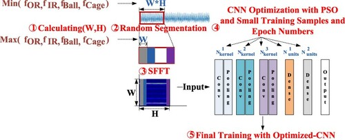
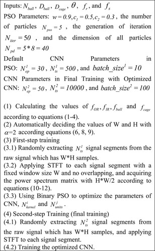
In this study, a self-adaptive CNN method based on STFT (SA-CNN) is proposed for bearing fault diagnosis, as shown in Figure 1. It has the following five steps: (1) calculating the input size (W, H); (2) randomly segmenting the raw signal to many signal segments with H*W points; (3) applying STFT to every signal segment, where the rectangle window size is W and has no overlapping, and obtaining the power spectrum with time–frequency information; (4) in the first-step training, PSO is used to evolve the CNN parameters, i.e. the numbers of kernels and dense units; (5) in the second-step training, the final training with optimized CNN is used to adjust the neuron weight.

Figure 1. Framework of SA-CNN.

2.1. Bearing fault types

Bearing faults are categorized into two types: generalized roughness fault and single-point fault (Eren, 2017; Stack et al., 2004).

The generalized roughness fault is a type of failure where the surface of a bearing has degraded considerably over a large area. It is a kind of distributed and noncyclic fault caused by improper lubrication, erosion, or pollution. There is no identifiable characteristic frequency associated with this fault type.

The single-point fault is a kind of single and localized fault caused by a small hole, a pit, or a missing material. As we all know, when a fault in one surfaces of a bearing strike another surface, a force impulse is generated, thus exciting resonances in the bearing and the machine. The successive impacts produce a series of impulse responses, the amplitude of which can be modulated (Ho & Randall, 2000). Therefore, the single-point fault creates a periodic impact vibration and produces a characteristic fault frequency.

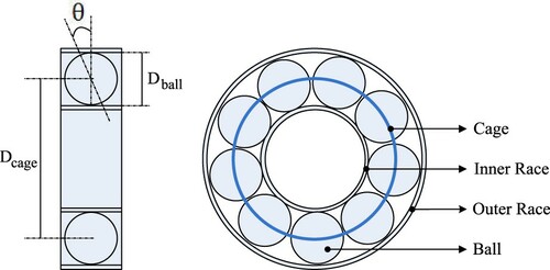
Since rolling-element bearings are constituted by an inner race, an outer race, a cage and balls, the single-point fault includes four types: cage fault, outer race fault, inner race fault and ball bearing fault, as shown in Figure 2 (Hamadache et al., 2015). Their corresponding characteristic fault frequencies are given by Equations (1–4) separately, where $N_{ball}$ is the number of balls in one bearing, $D_{ball}$ and $D_{cage}$ are the diameters of ball and cage respectively, $\theta$ is the contact angle, $f_r$ is the shaft speed, and $f_{\text{s}}$ is the sample frequency (Aimer et al., 2019; Eren, 2017). (1) $\begin{array}{rl}{f}_{OR}& =\frac{N_{ball}}{\text{2}}{f}_r\left(\text{1}-\frac{D_{ball}}{D_{cage}}\text{cos}\theta \right)\end{array}$(1) (2) $\begin{array}{rl}{f}_{IR}& =\frac{N_{ball}}{\text{2}}{f}_r\left(\text{1}+\frac{D_{ball}}{D_{cage}}\text{cos}\theta \right)\end{array}$(2) (3) $\begin{array}{rl}{f}_{ball}& =\frac{D_{cage}}{\text{2}{D}_{ball}}{f}_r\left(\text{1}-{\left(\frac{D_{ball}}{D_{cage}}\right)}^{\text{2}}\text{co}{\text{s}}^{\text{2}}\theta \right)\end{array}$(3) (4) $\begin{array}{rl}{f}_{cage}& =\frac{\text{1}}{\text{2}}{f}_r\left(\text{1}-\frac{D_{ball}}{D_{cage}}\text{cos}\theta \right)\end{array}$(4)

Figure 2. Bearing Components.

In addition, bearing characteristic fault frequencies can be grouped into four different zones: low frequency zone (shaft speed zone), bearing defect frequency zone, bearing nature resonance frequency zone, and high frequency zone in Figure 3 (El-Thalji & Jantunen, 2015).

Figure 3. Bearing frequency zones.

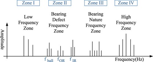
Bearing defect frequency zone (Zone II) include two parts. The first part is the low-frequency event which originates from the entry of the ball/roller in the vicinity of defect. This event gives peak in the bearing fault frequency zone. The second part is the high-frequency event, which is the result of the impact of rolling element on the trailing edge of the defect. The defect frequency zone can be derived from Equations (1–4) (Eren, 2017; Kumar & Kumar, 2019). To be notice, this study mainly focuses on the single-point fault or Zone II because the defect frequency will be used to auto decide the parameters related with STFT.

In signal-based methods, the major disadvantage of the time–frequency approach is that the computation time increases with both the number of samples and the number of sought harmonics. Equations (1–4) enable us to know in advance the frequency bands where the fault signature is likely to appear. Therefore, it can reduce the length of the spectrum and consequently the computation time (Aimer et al., 2019; Boudinar et al., 2016) to process the data on these predictable fault frequencies band instead of those on all the spectra.

2.2. STFT with auto-decided parameters

In Figure 1, when a raw signal is input, it will be segmented into many signal segments and every segment is applied with STFT. Therefore, the length of one signal segment and the window size are required to be fixed. As described in Figure 3 in Section 2.1, the bearing defect frequency zone contains lower frequency components and higher frequency components. To prevent any information loss of the lowest frequency component, the time of sampling L points must be longer than the multiple periods of the lowest frequency component, as in Equation (5). Correspondingly, L can be determined by Equation (6). Similarly, to capture the highest frequency component in the bearing defect frequency zone, the time of sampling W points must be longer than the multiple periods of the highest frequency component, as shown in Equation (7). Thus, W can be given by Equation (8). For Equations (5–8), $\alpha >2$ is required. (5) $\begin{array}{rl}{T}_L& =L/f_s>\alpha /\text{min}\left(\left[f_{OR},f_{IR},f_{ball},f_{cage}\right]\right)\end{array}$(5) (6) $\begin{array}{rl}L& >\alpha f_s/\text{min}\left(\left[f_{OR},f_{IR},f_{ball},f_{cage}\right]\right)\end{array}$(6) (7) $\begin{array}{rl}{T}_W& =W/f_s>\alpha /\text{max}\left(\left[f_{OR},f_{IR},f_{ball},f_{cage}\right]\right)\end{array}$(7) (8) $\begin{array}{rl}W& >\alpha f_s/\text{max}\left(\left[f_{OR},f_{IR},f_{ball},f_{cage}\right]\right)\end{array}$(8) (9) $\begin{array}{rl}H& =L/W\end{array}$(9)

After L samples are randomly extracted from the raw signal, they will be split into H frames, every of which has a fixed window size of W with no overlapping. Every frame with W samples is processed through FFT as Equation (10). Equation (12) is the normalization of the power spectrum. Since the power spectrum is symmetrical, only the single-sided data are fed into CNN, i.e. a matrix [H, W/2] is fed into CNN. (10) $\begin{array}{rl}{c}_{m,k}& =\frac{\text{1}}{W}\sum _{n=0}^{W-\text{1}}x\left(n\right)e^{-j\left(2pkn/W\right)}\end{array}$(10) (11) $\begin{array}{rl}{p}_{m,k}& =|c_{m,k}{|}^2\end{array}$(11) (12) $\begin{array}{rl}{p}_{m,k}& =\frac{p_{m,k}-\text{min}\left(p_m\right)}{\text{max}\left(p_m\right)-\text{min}\left(p_m\right)}\end{array}$(12) where $m\in \text{[0,H]}$, and $k\in \text{[0,W]}$.

2.3. Optimized CNN structure through PSO

2.3.1. Fixed CNN structure

Figure 4 illustrates the proposed CNN structure. Three successive convolution and pooling layers are used to extract high level features. The ReLU is taken as the activation function and the max pooling layer is for preserving the maximum coefficients that contain the main information of fault features. The last three dense layers construct an MLP as a classifier.

Figure 4. The proposed CNN structure.

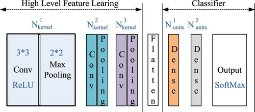
According to the universal approximation theorem, three-layer neuron network, with a sufficient number of hidden-layer units, can approximate any continuous function. But in practice learning, the hidden-layer units are hard to be determined. Feeding the auto extracted features with three-layer CNN into three-layer MLP can make MLP structure as simple as possible and PSO is used to find the optimal network structure, which maybe a wise solution.

In CNN, the loss function uses the categorical cross entropy loss (Zhang & Sabuncu, 2018); the optimizer is the Adam method because its hyper-parameters have intuitive interpretations and typically require little tuning (Kingma & Ba, 2015).

2.3.2. Binary PSO

In PSO, each particle has its own position x and velocity v and maintains a record of the position of its previous best performance $p_{best}$. A global best position $g_{best}$ is maintained by the algorithm. The $p_{best}$ represents potential solutions while the global best position is the global optimum solution.

The velocity v and the position x of each particle at the next iteration (t + 1) are calculated based on the values at current iteration (t). Each iteration comprises the evaluation of each particle, which is discussed in ‘(3) fitness evaluation’; each particle adjusts its own velocity in the direction of $p_{best}$ and $g_{best}$. Equation (15) is used for binary encoding. (13) $\begin{array}{rl}{v}_{t+\text{1}}& =w{v}_t+c_{\text{1}}{r}_{\text{1}}\left(p_{best}-x_t\right)+c_{\text{2}}{r}_{\text{2}}\left(g_{best}-x_t\right)\end{array}$(13) (14) $\begin{array}{rl}{x}_{t+\text{1}}& =x_t+v_{t+\text{1}}\end{array}$(14) (15) $\begin{array}{rl}{x}_{t+\text{1}}& =\left\{\begin{array}{cc}\text{0}& \text{rand()}\le f\left(v_{t+\text{1}}\right)\\ \text{1}& \text{otherwise}\end{array}\right.\end{array}$(15) (16) $\begin{array}{rl}f\left(y\right)& =\frac{\text{1}}{\text{1}+e^{-y}}\end{array}$(16) where w is called the ‘inertia weight’, which controls the impact of the previous velocity of the particle on its current one; $c_1$ and $c_2$ are positive constants with default values called ‘acceleration coefficients’; $r_1$, $r_2$ and rand() are random numbers uniformly distributed in the interval [0.0, 1.0] (Kennedy & Eberhart 1997; Ziani et al., 2017).

2.3.3. Fitness evaluation

Let all the kernel size be F, all the padding size be P, all the stride step be S, and all the pooling size be D. Then, the output size of one successive convolution and pooling layer can be expressed as: (17) $\begin{array}{rl}{W}_i& =\left(\left(W_{i-1}-F+2P\right)/S+1\right)/D\end{array}$(17) (18) $\begin{array}{rl}{H}_i& =\left(\left(H_{i-1}-F+2P\right)/S+1\right)/D\end{array}$(18)

The encoding information in each particle includes ${\text{N}}_{\text{kernel}}^{\text{i}}$ and ${\text{N}}_{\text{units}}^{\text{j}}\in \left\{0,\left[{\text{N}}_{\text{c}},2^{{\text{N}}_{\text{d}}}-1\right]\right\}$, where $\text{ i}\in \left[1,3\right],\text{j}\in \left[1,2\right]$, ${\text{N}}_{\text{c}}$ is the number of classes and ${\text{N}}_{\text{d}}=\text{8}$ is the number of bits in every dimension. Then, the fitness score can be expressed as Equation (20). (19) $\begin{array}{rl}\text{len}& =\frac{1}{\left({\sum }_{\text{i}=1}^3{N}_{\text{kernel}}^i{W}_{i-\text{1}}{H}_{i-\text{1}}\right)N_{\text{units}}^{\text{1}}+N_{\text{units}}^{\text{1}}{N}_{\text{units}}^{\text{2}}}\end{array}$(19) (20) $\begin{array}{rl}\text{score}& =\left\{\begin{array}{ll}\text{ - }acc& acc<\text{1}\\ \text{ - 1 - }len& acc=\text{1}\end{array}\right.\end{array}$(20) where acc is the prediction accuracy of CNN. It is noted that, to reduce the time complexity of PSO, a small number of training samples $N_{ts}$ and a small epoch number $N_{ep}$ are used to evaluate the prediction accuracy of each particle. Equation (19) is to ensure the simplicity of the network structure to reduce the time complexity.

2.4. Implementation of SA-CNN

In Figure 5, steps (1-2) are used to automatically decide the parameters of W and H used in STFT; steps (3.1-3.2) are implemented to preprocess STFT to generate the power spectrum matrix; step 3.3 is to optimize the CNN structure.

Figure 5. Procedure of SA-CNN.

3. Experiments

Two public famous fault diagnosis datasets, i.e. the Case Western Reserve University’s (CWRU) bearing dataset (Loparo & Loparo, 2013), and the Machinery Failure Prevention Technology (MFPT) society bearing fault dataset (Bechhoefer, 2016), are used to investigate the effectiveness of the proposed method. In every experiment, let the default batch size be 100 and the epoch number be 50. All results are obtained by running the algorithm for ten times with one GPU. The default proportion of the training data in the whole dataset Pt is 0.8. All prediction accuracies are from the results with the testing dataset.

3.1. CWRU bearing dataset

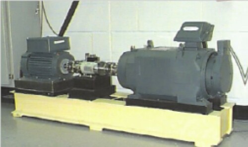
Two-horsepower reliance electric motors are used for the acquisition of accelerometer data on both the drive end (DE) and fan end (FE) bearings, as shown in Figure 6. In the experiment, artificial single-point faults are seeded in the bearing’s inner raceway (IR), outer raceway (OR), and rolling element (ball) (BF) with an electro discharge machining (EDM) operation. The vibration signal is sampled at 12 kHz through accelerometers attached at the 12 o’clock position to the DE of the motor.

Figure 6. Test bed for CWRU dataset.

Vibration data are recorded under various engine loads (0–3 hp) running at 1730, 1750, 1772, and 1797 RPM. The depth of the motor shaft bearings with faults ranges from 0 to 0.028 in. (0, 0.007, 0.014, 0.021, 0.028 in.), and the fault orientation includes the inner race, rolling element, and outer race. As shown in Table 1, all these data have one normal class and 15 fault classes without considering the different RPMs. Notably, in this study, some classes (bold and italic fonts) are merged as one value in the last column of Table 1. Hence, there are totally 12 classes of data to be classified. In this experiment, 10000 data samples are randomly extracted from the raw data file with the same probability.

Table 1. Classes in CWRU dataset.

Fault depth	Fault name	Class name used
0	Normal	Normal
0.028	0.028-Ball	28-Ball
	0.028-InnerRace	28-IR
0.021	0.021-Ball	21-Ball
	0.021-InnerRace	21-IR
	0.021-OuterRace12	21-OR
	0.021-OuterRace6
	0.021-OuterRace3
0.014	0.014-Ball	14-Ball
	0.014-InnerRace	14-IR
	0.014-OuterRace6	14-OR
0.007	0.007-Ball	07-Ball
	0.007-InnerRace	07-IR
	0.007-OuterRace3	07-OR
	0.007-OuterRace6
	0.007-OuterRace12

3.1.1. Comparison of the results from different methods

In this experiment, SA-CNN is compared with many deep learning methods including deep recurrent neural network (DRNN) (Jiang et al., 2018), sparse filter (Lei et al., 2016), CNN-Vibration image (Wen et al., 2018), CNN-PSO-WP (Fuan et al., 2017), CNN-Wavelet/STFT (Verstraete et al., 2017), HCNN (Wen et al., 2019b), and an optimized deep belief network with PSO (DBN-PSO) (Shao et al., 2015).

As can be seen from Table 2, our proposed SA-CNN method achieves an accuracy of 99.96% after running for ten times. Figure 7 shows one of the classification confusion matrixes. Furthermore, in our method, the number of classes to be classified is 12, which is more than that in other methods except DRNN (with an accuracy of 96.53%). Therefore, our method is more efficient than the other methods. ‘SA-CNN-E2E’ algorithm, called SA-CNN-End-to-End, means that there is no preprocessor of STFT before feeding into CNN. It get 99.60% accuracy, so the preprocessor of STFT is valuable to improve the algorithm performance.

Figure 7. A classification confusion matrix (DE_time).

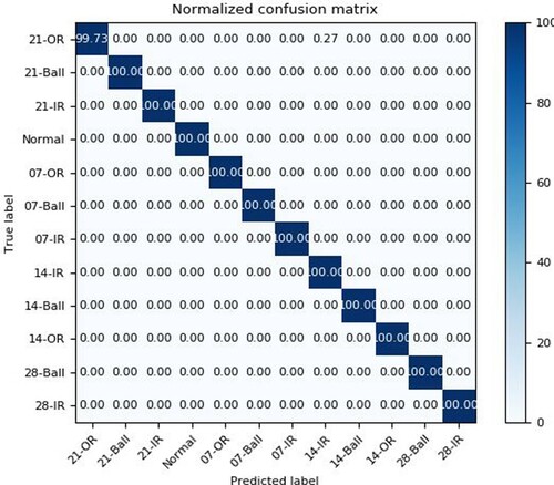
Table 2. Comparison with CWRU dataset (${\text{N}}_{\text{ep}}=30$, ${\text{N}}_{\text{ts}}=500$, DE_time, %).

Algorithm	Average accuracy	Class number
SA-CNN	99.96	12
SA-CNN-E2E	99.60	12
DRNN (Jiang et al., 2018)	96.53	12
HCNN (Wen et al., 2019)	99.82	10
CNN-Vibration image (Wen et al., 2018)	99.79	10
Sparse filter (Lei et al., 2016)	99.66	10
CNN-PSO-WP (Fuan et al., 2017)	99.71	8
CNN- Wavelet 96×96 (Verstraete et al., 2017)	99.8	4
CNN-STFT96×96 (Verstraete et al., 2017)	99.5	4
DBN-PSO (Shao et al., 2015)	87.45	-

3.1.2. Spectrum image

According to Equations (1–9) and the parameter settings ($f_s=\text{12000}$, $\alpha =\text{2}$, $rpm\approx \text{1700}$, $D_{ball}=\text{0}\text{.3126}$, $D_{cage}=\text{1}\text{.537}$, $\theta =\text{0}$, $N_{ball}=\text{9}$, and $f_r=\text{1700/60}$), we can get the characteristic vibration frequencies as follows: $f_{OR}=\frac{\text{9}}{\text{2}}{f}_r\left(\text{1 - }\frac{\text{0}\text{.3126}}{\text{1}\text{.537}}\text{cos}\theta \right)=\text{3}\text{.585}{f}_r$ $f_{IR}=\frac{\text{9}}{\text{2}}{f}_r\left(\text{1 + }\frac{\text{0}\text{.3126}}{\text{1}\text{.537}}\text{cos}\theta \right)=\text{5}\text{.415}{f}_r$ $f_{ball}=\frac{\text{1}\text{.537}}{2\ast 0\text{.3126}}{f}_r\left(\text{1 - }{\left(\frac{\text{0}\text{.3126}}{\text{1}\text{.537}}\right)}^{\text{2}}\text{co}{\text{s}}^{\text{2}}\theta \right)=\text{2}\text{.357}{f}_r$ $f_{cage}=\frac{\text{1}}{\text{2}}{f}_r\left(\text{1 - }\frac{\text{0}\text{.3126}}{\text{1}\text{.537}}\text{cos}\theta \right)=\text{0}\text{.3983}{f}_r$ $L>\text{2}\frac{\text{12000}}{\text{min}\left(\text{3}\text{.585,5}\text{.415,2}\text{.357,0}\text{.3983}\right)\ast \frac{\text{1700}}{\text{60}}}\text{ = 2126}\text{.69}$ $\begin{array}{rl}W& >\text{2}\frac{\text{12000}}{\text{max}\left(\text{3}\text{.585,5}\text{.415,2}\text{.357,0}\text{.3983}\right)\ast \frac{\text{1700}}{\text{60}}}\text{ = 156}\text{.43}\\ L& =\text{2127},W=\text{157},H=L/W=\text{14}\end{array}$

As Table 3 shows, the spectrum images with STFT according to equations (10-12) are easy to be discriminated by human eyes. Table 4 lists all error results found in the experiment and the corresponding activation maps (Selvaraju et al., 2017). In these activation maps, the maximum coefficients are always mapped to high temperatures in the heat map. In Table 4, 21-OR and 14-IR are the most difficult to be discriminated. Moreover, 14-IR and 14-OR, or 21-Ball and 07-OR are similar in the high temperature area if the location is not considered. The main reason is that: the convolutional units of various layers of CNNs actually behave as object detectors (Zhou et al., 2015), but this ability is lost when fully-connected layers are used for classification (Zhou et al., 2016).

Table 3. Signal and spectrum.

Table 4. Class activation mapping.

3.1.3. Performance and parameters

As the CNN structure is optimized with PSO, the time complexity needs to be considered carefully. For analysing the performance with different parameters, our method is implemented with different combinations between $N_{ep}=\left[30,50,70\right]$ and $N_{ts}=\left[500,1500,2500\right]$

In Tables 5 and 6, the combinations of $(N_{ep}=70,N_{ts}=500)$ and $\left(N_{ep}=30,N_{ts}=1500\right)$ can get better prediction accuracies, but their time complexity is not the minimum value. Hence, there is a balance choice between time complexity and prediction accuracy. Of course, the time complexity should be considered only in the beginning of the CNN optimization with PSO, and it will be the same as existing CNN methods once the optimized CNN is fixed.

Table 5. Prediction accuracies with different parameters (DE_time, %).

$N_{ep}$	$N_{ts}$	Min	Max	Mean	Std
30	500	99.85	100.00	99.96	0.05
50	500	99.90	100.00	99.98	0.04
70	500	99.95	100.00	99.99	0.02
30	1500	99.95	100.00	99.99	0.02
30	2500	99.90	100.00	99.98	0.03

Table 6. Time complex with CWRU dataset (DE_time).

$N_{ts}\left(N_{ep}=30\right)$	Time (s)	$N_{ep}\left(N_{ts}=500\right)$	Time (s)
500	2608.039835	30	2608.039835
1500	11780.00252	50	3484.697968
2500	24919.51808	70	8972.817968

Furthermore, according to Table 6, $N_{ts}$ is the main factor that leads to the higher time complexity.

3.1.4. Evolution of CNN with PSO

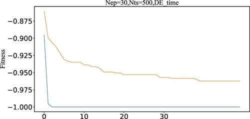
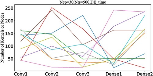
Figure 8 depicts the curves related with the converge speed, which is proportional to $N_{ep}$ and $N_{ts}$. The bottom figure is a partially enlarged figure. The fitness value −1 means that the prediction accuracy is 100% according to Equation (20). After the fitness value reaches to −1, the converging speed becomes slowly because of the huge searching space. Furthermore, the optimization of CNN is a multi-optimization problem as the CNN structure from different running results is different (Figure 9).

Figure 8. Fitness curves (bottom: partially enlarged figure).

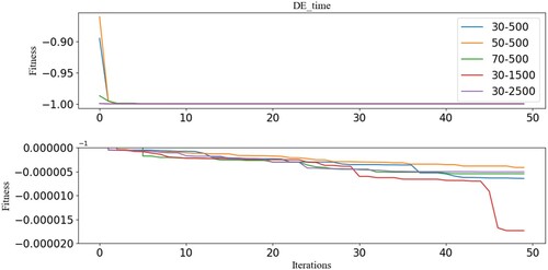
Figure 9. Network structure.

3.1.5. Effect of STFT

As Figure 10 shown, with the preprocessing of STFT, the fitness can be quickly converged to −1.0. Therefore, signal processing taken as a preprocessing method to extract basic time–frequency information can accelerate the evolution of PSO and improve the algorithm performance.

Figure 10. Fitness curve.

3.2. MFPT bearing dataset

This MFPT dataset is recorded from a bearing test rig (normal bearing data, an outer race fault under various loads, and an inner race fault under various loads), and includes four sets of bearing vibration data: (1) a baseline set under the load of 270 lbs, which is sampled at 97656 Hz for 6 s; (2) an outer race fault set including three outer race faults (ThreeOR) under the load of 270 lbs, which are sampled at 97656 Hz for 6 s; (3) seven additional outer race faults (SevenOR) under various loads of 25, 50, 100, 150, 200, 250, and 300 lbs, which are sampled at 48828 Hz for 3 s; and (4) seven inner race faults (SevenIR) under various loads of 25, 50, 100, 150, 200, 250, and 300 lbs, which are sampled at 48828 Hz for 3 s. In the experiments, 10000 data samples are randomly extracted from the raw data file with the same probability.

3.2.1 Spectrum image

According to Equations (1–9) and the parameter settings ($f_s=\text{97656/6}$, $\alpha =\text{2}$, $D_{ball}=\text{0}\text{.235}$, $D_{cage}=\text{1}\text{.245}$, $\theta =\text{0}$, $N_{ball}=\text{8}$, and $f_r=\text{25}$), we can get the characteristic vibration frequencies as follows: $f_{OR}=\frac{\text{8}}{\text{2}}{f}_r\left(\text{1}-\frac{\text{0}\text{.235}}{\text{1}\text{.245}}\text{cos}\theta \right)=\text{3}\text{.245}{f}_r$ $f_{IR}=\frac{\text{8}}{\text{2}}{f}_r\left(\text{1 + }\frac{\text{0}\text{.235}}{\text{1}\text{.245}}\text{cos}\theta \right)=\text{4}\text{.755}{f}_r$ $f_{ball}=\frac{\text{1}\text{.245}}{2\ast 0\text{.235}}{f}_r\left(\text{1}-{\left(\frac{\text{0}\text{.235}}{\text{1}\text{.245}}\right)}^{\text{2}}\text{co}{\text{s}}^{\text{2}}\theta \right)=\text{2}\text{.555}{f}_r$ $f_{cage}=\frac{\text{1}}{\text{2}}{f}_r\left(\text{1}-\frac{\text{0}\text{.235}}{\text{1}\text{.245}}\text{cos}\theta \right)=\text{0}\text{.406}{f}_r$ $L>\text{2}\ast \frac{\text{97656/6}}{\text{min}\left(\text{3}\text{.245,4}\text{.755,2}\text{.555,0}\text{.406}\right)\ast 25}\text{ = 3207}\text{.09}$ $\begin{array}{rl}W& >\text{2}\ast \frac{\text{97656/6}}{\text{max}\left(\text{3}\text{.245,4}\text{.755,2}\text{.555,0}\text{.406}\right)\ast 25}\text{ = 273}\text{.83}\\ L& =\text{3208},W=\text{274},H=L/W=\text{12}\end{array}$

Table 7 gives the signals and spectrum images used by our method according to Equations (10–12). It seems that the spectrum imaged can be readily discriminated by human eyes.

Table 7. Signals and spectra.

3.2.2. Comparison of the results from different methods

In Table 8, it can be seen that our proposed method achieves an accuracy of 99.99% for 4 classes and 100% for 3 class classification. By contrast, CNN using the time–frequency information of wavelet or spectrogram does not perform well because of the non-optimized CNN structure and the parameters used in signal processing (Verstraete et al., 2017; Wen et al., 2019).

Table 8. Comparison with MFPT dataset (Pt=0.8, %).

Algorithm	Average accuracy	Class number
SA-CNN	99.99	4
SA-CNN	100.0	3
CNN- Wavelet 96 × 96 (Verstraete et al., 2017)	99.9	3
CNN-Spectrogram 96 × 96 (Wen et al., 2019b)	91.3	3
CNN-HHT 96 × 96 (Sohaib et al., 2017)	92.9	3
CNN-VAE (Wen et al., 2019)	92.58	3
SECNN (Wen et al., 2019b)	99.94	3

3.3. Discussion

All results within the ten running times are merged into Tables 9 and 10, which provides the probability of achieving an accuracy of 100% with stable standard deviations. In Table 9, larger $N_{ep}$ leads to higher stability and larger probability, whereas larger $N_{ts}$ leads to worse performance of the method. For example, when $N_{ts}=500$ and $N_{ep}$ is increased, the value of ‘std’ decreases and the value of ‘probability’ mostly increases; when $N_{ep}=30$ and $N_{ts}$ is increased, the value of ‘std’ mostly increases. This is because that larger $N_{ts}$ makes PSO require more time to converge to the stable level. Therefore, $N_{ep}$ is a main factor to be tuned. Notably, according to section 3.1.3, larger $N_{ep}$ may lead to more training time. In Table 10, larger ‘batch_size’ make the prediction accuracy less ‘std’ and more stable.

Table 9. Prediction accuracies with different parameters (%).

Data	$N_{ep}$	$N_{ts}$	Mean	Std	Probability (100)
CWRU-DE	30	500	99.96	0.05	0.5
	50	500	99.98	0.04	0.8
	70	500	99.99	0.02	0.8
	30	1500	99.99	0.02	0.8
	30	2500	99.98	0.03	0.8
MFPT	30	500	99.99	0.03	0.8
	50	500	99.99	0.02	0.9
	70	500	100	0	1
	30	1500	99.99	0.03	0.8
	30	2500	99.04	3.75	0.6

Table 10. The influence of different batch size (%).

Batch_Size	Mean	Std	Probability (100)
10	99.96	0.05	0.5
50	99.97	0.005	0.6
100	99.97	0.003	0.6

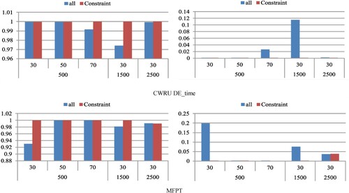
In Figure 11, the left figures (no any constraint) have more numbers near zero, and the network structure converges to simpler network structure with less neuron nodes because the fitness function considers the simplicity of network structure in Equation (19). Consequently, the simple network structure may lead to worse performance in terms of both prediction accuracy and its standard deviation, as shown in Figure 12.

Figure 11. Comparison of network structure.

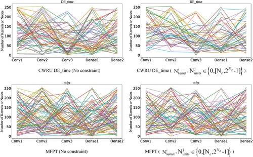
Figure 12. Comparison of network structure (Left: prediction accuracy; right: standard deviation).

4. Conclusions

In summary, a self-adaptive CNN method (SA-CNN) with two-step training is proposed on account of the time-consuming problem in the design of a CNN structure or its parameter tuning. To reduce the time complexity, two main mechanisms are used. First, the CNN structure is fixed, and only its key parameters including the kernel number and the number of neuron nodes are optimized by PSO. Second, a small number of training samples and a small epoch number are used to evaluate the prediction accuracy. Based on the given the bearing parameters, SA-CNN can automatically decide the parameters of W and H used in STFT, and adjust CNN into an optimized structure. Therefore, the proposed method can be easily applied in industry. Through the experiments with two famous public datasets, CWRU and MFPT, it is demonstrated that the SA-CNN method can achieve better results than other state-of-art methods and the preprocessing of STFT can accelerate the evolution speed of PSO. In the future, the location of high temperature area in the rotating machinery will be considered to improve the prediction accuracy; meanwhile, it is necessary to take both fault patterns and fault deterioration into account.

Acknowledgements

This work was supported in part by the National Natural Science Foundation of China (61502423), Zhejiang Provincial Natural Science Foundation (LY16G020012), and Zhejiang Province Public Welfare Technology Application Research(LGF19F010-002, LGF20F010004, LGG21F030014:The Research on Cold-Start Fault Diagnosis Method Based on Immune Algorithm and Deep Learning).

Disclosure statement

No potential conflict of interest was reported by the author(s).

Additional information

Funding

This work was supported in part by the National Natural Science Foundation of China (61502423), Zhejiang Provincial Natural Science Foundation [grant number LY16G020012], and Zhejiang Province Public Welfare Technology Application Research Project [grant numbers LGF19F010002, LGF20F010004, LGG21F030014].

References

- Aimer, A. F., Boudinar, A. H., Benouzza, N., et al. (2019). Bearing fault diagnosis of a PWM inverter fed-induction motor using an Improved short time Fourier Transform. Journal of Electrical Engineering & Technology, 1–10. https://doi.org/https://doi.org/10.1007/s42835-019-00096-y
- Bechhoefer, E. (2016). A quick introduction to bearing envelope analysis. MFPT Data, http://www.mfpt.org/FaultData/Fault-Data.htm.Set
- Boudinar, A. H., Benouzza, N., Bendiabdellah, A., & Khodja, M.-E.-A. (2016). Induction motor bearing fault analysis using a root-MUSIC method. IEEE Transactions on Industry Applications, 52(5), 3851–3860. https://doi.org/https://doi.org/10.1109/TIA.2016.2581143
- Chen, Z., & Li, W. (2017). Multisensor feature fusion for bearing fault diagnosis using sparse autoencoder and deep belief network. IEEE Transactions on Instrumentation and Measurement, 66(7), 1693–1702. https://doi.org/https://doi.org/10.1109/TIM.2017.2669947
- Chen, F., Tang, B., Song, T., & Li, L. (2014). Multi-fault diagnosis study on roller bearing based on multi-kernel support vector machine with chaotic particle swarm optimization. Measurement, 47, 576–590. https://doi.org/https://doi.org/10.1016/j.measurement.2013.08.021
- El-Thalji, I., & Jantunen, E. (2015). Fault analysis of the wear fault development in rolling bearings. Engineering Failure Analysis, 57, 470–482. https://doi.org/https://doi.org/10.1016/j.engfailanal.2015.08.013
- Eren, L. (2017). Bearing fault detection by one-dimensional convolutional neural networks. Mathematical Problems in Engineering. https://doi.org/https://doi.org/10.1155/2017/8617315.
- Fuan, W., Hongkai, J., Haidong, S., Wenjing, D., & Shuaipeng, W. (2017). An adaptive deep convolutional neural network for rolling bearing fault diagnosis. Measurement Science and Technology, 28(9), 095005. https://doi.org/https://doi.org/10.1088/1361-6501/aa6e22
- Gao, Z., Ding, S. X., & Cecati, C. (2015). Real-time fault diagnosis and fault-tolerant control. IEEE Transactions on Industrial Electronics, 62(6), 3752–3756. https://doi.org/https://doi.org/10.1109/TIE.2015.2417511
- Hamadache, M., Lee, D., & Veluvolu, K. C. (2015). Rotor speed-based bearing fault diagnosis (RSB-BFD) under variable speed and constant load. IEEE Transactions on Industrial Electronics, 62(10), 6486–6495. https://doi.org/https://doi.org/10.1109/TIE.2015.2416673
- Harmouche, J., Delpha, C., & Diallo, D. (2015). Improved fault diagnosis of ball bearings based on the global spectrum of vibration signals. IEEE Transactions on Energy Conversion, 30(1), 376–383. https://doi.org/https://doi.org/10.1109/TEC.2014.2341620
- Ho, D., & Randall, R. B. (2000). Optimisation of bearing diagnostic techniques using simulated and actual bearing fault signals. Mechanical Systems and Signal Processing, 14(5), 763–788. https://doi.org/https://doi.org/10.1006/mssp.2000.1304
- Hoang, D. T., & Kang, H. J. (2019). Rolling element bearing fault diagnosis using convolutional neural network and vibration image. Cognitive Systems Research, 53, 42–50. https://doi.org/https://doi.org/10.1016/j.cogsys.2018.03.002
- Huo, Z., Zhang, Y., Francq, P., Shu, L., & Huang, J. (2017). Incipient fault diagnosis of roller bearing using optimized wavelet transform based multi-speed vibration signatures. IEEE Access, 5, 19442–19456. https://doi.org/https://doi.org/10.1109/ACCESS.2017.2661967
- Jia, F., Lei, Y., Lin, J., Zhou, X., & Lu, N. (2016). Deep neural networks: A promising tool for fault characteristic mining and intelligent diagnosis of rotating machinery with massive data. Mechanical Systems and Signal Processing, 72-73, 303–315. https://doi.org/https://doi.org/10.1016/j.ymssp.2015.10.025
- Jiang, H., Li, X., Shao, H., & Zhao, K. (2018). Intelligent fault diagnosis of rolling bearings using an improved deep recurrent neural network. Measurement Science and Technology, 29(6), 065107. https://doi.org/https://doi.org/10.1088/1361-6501/aab945
- Jung, U., & Koh, B.-H. (2015). Wavelet energy-based visualization and classification of high-dimensional signal for bearing fault detection. Knowledge and Information Systems, 44(1), 197–215. https://doi.org/https://doi.org/10.1007/s10115-014-0761-z
- Kennedy, J., & Eberhart, R. C. (1997). A discrete binary version of the particle swarm optimisation algorithm. In James M. Tien (Ed.), Proceedings of the IEEE International Conference on neural networks (pp. 4104–4108). IEE.
- Kingma, D. P., & Ba, J. (2015). Adam: A method for stochastic optimization. International Conference on learning representations.
- Kumar, A., & Kumar, R. (2019). Role of signal processing, modeling and decision making in the diagnosis of rolling element bearing defect: A review. Journal of Nondestructive Evaluation, 38(1). https://doi.org/https://doi.org/10.1007/s10921-018-0543-8
- Lei, Y., Jia, F., Lin, J., Xing, S., & Ding, S. X. (2016). An intelligent fault diagnosis method using unsupervised feature learning towards mechanical big data. IEEE Transactions on Industrial Electronics, 63(5), 3137–3147. https://doi.org/https://doi.org/10.1109/TIE.2016.2519325
- Lin, H. C., & Ye, Y. C. (2019). Reviews of bearing vibration measurement using fast Fourier transform and enhanced fast Fourier transform algorithms. Advances in Mechanical Engineering, 11(1). https://doi.org/https://doi.org/10.1177/1687814018816751.
- Liu, H., Li, L., & Ma, J. (2016). Rolling bearing fault diagnosis based on STFT-deep learning and sound signals. Shock and Vibration. https://doi.org/https://doi.org/10.1155/2016/6127479.
- Loparo, K. A., & Loparo, K. A. (2013). Bearing data center. Case Western Reserve University, http://csegroups.case.edu/bearingdatacenter/pages/welcome-case-western-reserve-university-bearing-datacenter-website
- Ma, J., Wu, J., & Wang, X. (2018). Incipient fault feature extraction of rolling bearings based on the MVMD and Teager energy operator. ISA Transactions, 80, 297–311. https://doi.org/https://doi.org/10.1016/j.isatra.2018.05.017
- Peng, Y., Wen, Z., Li, D., & Shang, Z. (2017). A new deep learning model for fault diagnosis with good anti-noise and domain adaptation ability on raw vibration signals. Sensors, 17(2), 387–425. https://doi.org/https://doi.org/10.3390/s17020387
- Qian, W., Li, S., Wang, J., et al. (2018). An intelligent fault diagnosis framework for raw vibration signals: Adaptive overlapping convolutional neural network. Measurement Science and Technology, 29(9). https://doi.org/https://doi.org/10.1088/1361-6501/aad101
- Rai, A., & Upadhyay, S. H. (2016). A review on signal processing techniques utilized in the fault diagnosis of rolling element bearings. Tribology International, 96, 289–306. https://doi.org/https://doi.org/10.1016/j.triboint.2015.12.037
- Selvaraju, R. R., Cogswell, M., Das, A., et al. (2017). Grad-cam: Visual explanations from deep networks via gradient-based localization. Proceedings of the IEEE International Conference on Computer Vision, 618–626. doi: https://doi.org/10.1109/ICCV.2017.74
- Seshadrinath, J., Singh, B., & Panigrahi, B. K. (2014). Vibration analysis based interturn fault diagnosis in induction machines. IEEE Transactions on Industrial Informatics, 10(1), 340–350. https://doi.org/https://doi.org/10.1109/TII.2013.2271979
- Shao, H., Jiang, H., Zhang, X., & Niu, M. (2015). Rolling bearing fault diagnosis using an optimization deep belief network. Measurement Science and Technology, 26(11). https://doi.org/https://doi.org/10.1088/0957-0233/26/11/115002
- Sohaib, M., Kim, C. H., & Kim, J. M. (2017). A hybrid feature model and deep-learning-based bearing fault diagnosis. Sensors, 17(12), 2876. https://doi.org/https://doi.org/10.3390/s17122876
- Soualhi, A., Medjaher, K., & Zerhouni, N. (2015). Bearing health monitoring based on Hilbert–huang transform, support vector machine, and regression. IEEE Transactions on Instrumentation and Measurement, 64(1), 52–62. https://doi.org/https://doi.org/10.1109/TIM.2014.2330494
- Stack, J. R., Habetler, T. G., & Harley, R. G. (2004). Fault classification and faultsignature production for rolling element bearings in electric machines. IEEE Transactions on Industry Applications, 40(3), 735–739. https://doi.org/https://doi.org/10.1109/TIA.2004.827454
- Verstraete, D., Ferrada, A., Droguett, E. L., et al. (2017). Deep learning enabled fault diagnosis using time-frequency image analysis of rolling element bearings. Shock and Vibration. https://doi.org/https://doi.org/10.1155/2017/5067651
- Wang, D. (2016). K-nearest neighbors based methods for identification of different gear crack levels under different motor speeds and loads: Revisited. Mechanical Systems and Signal Processing, 70-71, 201–208. https://doi.org/https://doi.org/10.1016/j.ymssp.2015.10.007
- Wang, X. B., Yang, Z. X., & Yan, X. A. (2018). Novel particle swarm optimization-based variational mode decomposition method for the fault diagnosis of complex rotating machinery. IEEE/ASME Transactions on Mechatronics, 23(1), 68–79. doi: https://doi.org/10.1109/ISFA.2016.7790137
- Wang, J., Zhuang, J., Duan, L., & Cheng, W. (2016). A multi-scale convolution neural network for featureless fault diagnosis. Proceedings of the International Symposium on Flexible Automation, 65–70. doi: https://doi.org/10.1109/ISFA.2016.7790137
- Wen, L., Gao, L., & Li, X. (2019a). A New Snapshot Ensemble convolutional neural network for fault diagnosis. IEEE Access, 1–11. https://doi.org/https://doi.org/10.1109/access.2019.290329
- Wen, L., Li, X., & Gao, L. (2019b). A New Two-level Hierarchical diagnosis network based on convolutional neural network. IEEE Transactions on Instrumentation and Measurement, 1–9. https://doi.org/https://doi.org/10.1109/TIM.2019.2896370
- Wen, L., Li, X., Gao, L., & Zhang, Y. (2018). A new convolutional neural network-based data-driven fault diagnosis method. IEEE Transactions on Industrial Electronics, 65(7), 5990–5998. https://doi.org/https://doi.org/10.1109/TIE.2017.2774777
- Yi, C., Lv, Y., & Dang, Z. (2016). A fault diagnosis scheme for rolling bearing based on particle swarm optimization in variational mode decomposition. Shock and Vibration. https://doi.org/https://doi.org/10.1155/2016/9372691
- Yuan, Z., Zhang, L., & Duan, L. (2018). A novel fusion diagnosis method for rotor system fault based on deep learning and multi-sourced heterogeneous monitoring data. Measurement Science and Technology, 29(11). https://doi.org/https://doi.org/10.1088/1361-6501/aadfb3
- Yuwono, M., Qin, Y., Zhou, J., Guo, Y., Celler, B. G., &Su, S. W. (2016). Automatic bearing fault diagnosis using particle swarm clustering and hidden Markov model. Engineering Applications of Artificial Intelligence, 47, 88–100. https://doi.org/https://doi.org/10.1016/j.engappai.2015.03.007
- Zhang, X., Liang, Y., Zhou, J., & Zang, Y. (2015). A novel bearing fault diagnosis model integrated permutation entropy, ensemble empirical mode decomposition and optimized SVM. Measurement, 69, 164–179. https://doi.org/https://doi.org/10.1016/j.measurement.2015.03.017
- Zhang, Z., & Sabuncu, M. (2018). Generalized cross entropy loss for training deep neural networks with noisy labels. Advances in Neural Information Processing Systems, 8778–8788. https://dl.acm.org/doi/https://doi.org/10.5555/3327546.3327555
- Zhou, B., Khosla, A., Lapedriza, A., et al. (2016). Learning deep features for discriminative localization. Proceedings of the IEEE Conference on Computer Vision and Pattern Recognition.
- Zhou, B., Khosla, A., Lapedriza, A., Oliva, A., & Torralba, A. (2015). Object detectors emerge in deep scene cnns. International Conference on Learning Representations.
- Ziani, R., Felkaoui, A., & Zegadi, R. (2017). Bearing fault diagnosis using multiclass support vector machines with binary particle swarm optimization and regularized Fisher’s criterion. Journal of Intelligent Manufacturing, 28(2), 405–417. https://doi.org/https://doi.org/10.1007/s10845-014-0987-3