Robust adaptive fuzzy control for single-chamber single-population microbial fuel cell

Abstract

Energy supply from renewable sources is one of the most attractive fields of study in recent years. Ensuring the efficient operation of the microbial fuel cell (MFC) due to its capabilities requires the development of appropriate control strategies. This paper presents a combination of fuzzy and adaptive control methods to control single-chamber single-population MFC. For estimating nonlinear terms as well as the parametric uncertainty in the model, fuzzy approximation method has been used and the effects of disturbances as well as fuzzy approximation gains have been covered by adaptive method. Using Liapunov theory, the robust stability of the system under the proposed controller is shown. The simulation results clearly show the ability of the proposed method to achieve MFC control goals.

KEYWORDS:

• Microbial fuel cell
• adaptive fuzzy control
• robust stability
• renewable energy

1. Introduction

Energy growth is directly related to the development and prosperity around the world. Responding to the growing demand for energy safely and without harming the environment is a major challenge. Increasing energy production is important to help economic and social progress and to create a better quality of life, especially in developing countries. Reliable and affordable energy is a basic need for all countries. Reliable energy supports the development of industry, modern agriculture, increased trade and better transportation. Today, most of the world’s energy needs come from hydrocarbons, and despite of significant advances in energy efficiency, global energy demand is expected to increase by about 25% from 2020 to 2040 (Capuano, 2018; Newell et al., 2016). All energy production must increase to meet this growing demand and renewable have a vital role in this regard.

Renewable energies are clean, endless and increasingly competitive energy resources. They are very different from fossil fuels in terms of variety, frequency and potential for use anywhere on the planet, but most importantly, they do not produce greenhouse gases and do not emit any pollutants. Their costs are also declining and at a stable rate, while the overall cost of fossil fuels is in the opposite direction despite of their current fluctuations. Developing clean energy is critical to combating climate change and limiting its devastating effects. Renewable energies include: wind energy, solar energy, hydraulic or hydroelectric energy, biomass and biogas, geothermal energy, tidal energy, wave energy, bioethanol, biodiesel (Anaza et al., 2017; Atabani et al., 2012; Cheng, 2017; Kannan & Vakeesan, 2016; Murthy & Rahi, 2017; Olasolo et al., 2016; Sun et al., 2018; Wilberforce et al., 2019).

One possible energy source is the use of microbial fuel cells (MFCs). Using MFC as an alternative source of electricity generation is a safe, clean and efficient process that uses renewable methods and does not produce any toxic by-products. MFCs follow the same concept of traditional fuel cells. However, MFCs use the bio-catalytic capabilities of viable microorganisms and are able to use a wide range of organic fuel sources to generate electricity by converting energy stored in chemical bonds (Slate et al., 2019). Microorganisms, such as bacteria, can produce electricity by using organic matter and biodegradable substrates such as wastewater, whilst obtain biodegradation/treatment of biodegradable products, such as municipal wastewater (Habermann & Pommer, 1991; Slate et al., 2019).

Obviously, due to the working conditions of the environment and the types of degradable substrates, much attention has been paid to MFCs. The microbial fuel cell reduces carbon dioxide to generate electricity and is not only a renewable energy source, but also uses additional carbon dioxide to rebuild fuels and reduces environmental pollutants such as wastewater.

However, the MFC voltage can change dramatically due to environmental and operating conditions that can affect their efficiency and performance. Control of MFCs is very beneficial, as it is expected to improve disturbance rejection and increase relative stability in a power management system which can lead to improved cell performance. MFCs are all subject to additional changes in electrical load as an input disturbance in the operating voltage range for different MFC designs (Boghani et al., 2013, 2016). Their maximum produced power are highly dependent on external disturbances such as variations of the inlet substrate concentration, the anodic compartment temperature or the pH concentration that attenuate their performance significantly (Chae et al., 2009). Therefore, the use of a real-time control method is essential for MFC to achieve maximum performance despite external disturbances. The MFC controller must be able to maintain the output voltage within an acceptable range while overcoming the disturbances in the system.

The next issue in addition to the disturbance is the uncertainty of the parameter as well as the nonlinear term in the models provided for the microbial fuel cell. Due to the weakness of the linear controllers as well as the non-linear ones that have been used to date, the necessary measures must be taken in this regard.

To date, various controllers have been used based on the mathematical model of the MFC system. Input-output linearization methods are limited in properly representing the correct dynamics of nonlinear systems in the wide operating range (Chen et al., 1995; Dochain, 1992). Nonlinear control schemes can handle system uncertainty and online parameter estimation. A fuzzy PID controller for constant output voltage of MFC is discussed in Yan and Fan (2013). Lipping et al. presented a predictive model control scheme (MPC) for a two-chamber microbial fuel cell (Fan et al., 2015). Lately, the adaptive control technique has taken considerable attention to overcome the limitation that the nonlinearities of considered systems are required to be identified or can be linearly parameterized. A new adaptive sliding mode control scheme for covering disturbances and uncertainty effects in single-chamber microbial fuel cells is presented in Fu et al. (2020). In addition, uncertain nonlinear systems can be modelled by combining fuzzy set theory with fuzzy equations. Because the uncertainty in nonlinear systems can be turned into fuzzy set theory, fuzzy systems are good models for systems with uncertainty. Fuzzy models are made according to fuzzy rules, and these rules provide information about uncertain nonlinear systems. Each nonlinear system can be approximated by several piecewise linear systems (Takagi–Sugeno fuzzy model) or known nonlinear systems (Mamdani fuzzy model) (Mamdani, 1974; Takagi & Sugeno, 1985). Uncertain nonlinear systems can be modelled by fuzzy models with simple linear or nonlinear models.

Accordingly, in this study, adaptive fuzzy controller is used to control MFC in order to cover the effects of nonlinear terms, parameter uncertainty, and disturbance. First, the nonlinear model of the single-chamber single-population MFC is considered. In this section, it is assumed that there is a parametric uncertainty in the model and also the disturbance is limited to the upper bound, but we have no knowledge about its value. Using the fuzzy method, we approximate the nonlinear (rigid) part and the uncertainty of the system with fuzzy membership functions. Adaptive methods have also been used to obtain the fuzzy approximator weights and to eliminate the effects of boundary perturbation with an unknown upper bound. Finally, the robust stability of the proposed method is demonstrated under Lyapunov theory. In general, the innovations of the article are as follows:

1. Consider a nonlinear model of the system in the presence of perturbations and uncertainties.

2. The use of fuzzy methods to approximate the non-linear terms and uncertainties.

3. Using an adaptive method to cover the effects of perturbation on the system.

4. Combining fuzzy and adaptive methods to ensure system stability and control under different operating conditions.

Accordingly, the article format is as follows: The second part describes the nonlinear MFC model used for the system. Section 3 describes the proposed control method and Section 4 discusses four scenarios for simulation results and finally the conclusion is presented in Section 5.

2. Single-chamber single-population microbial fuel cell mathematical model

Essential parts of MFCs are anode, cathode, media (substrate), membrane and microorganisms. Figure 1 shows the basic construction of microbial fuel cell. Existing bacteria in anode chamber produce protons and electrons by utilizing substrates like acetate, glucose, lactate, nitrilotriacetic acid, ribitol, glucuronic acid, cysteine, etc. (Pant et al., 2010). Produced electrons are directly or indirectly moved to the anode. Direct electron move occurs through nanowires or intracellular mediator and biofilm created at anode surface (Lovley, 2008). An external mediator is added to move electrons from bacteria to anode, which is known as the backhanded method to move electrons (Lovley, 2006). Commonly, Shewanella putrefaciens, G. Sulferredunces, G. Metallireducens, Rhodoferax ferrieducens, E. Coli, Sreptococcus lactis, Proteus vulgaris and Pseudomonas bacteria are utilized in MFCs (Choudhury et al., 2017). Electrons are moved from anode to cathode by means of an outside circuit. Protons are moved from anode to cathode through proton exchange membrane (PEM). Electrons and protons join at cathode, make fresh water and generate power from wastewater.

Figure 1. Single-chamber MFC with PEM.

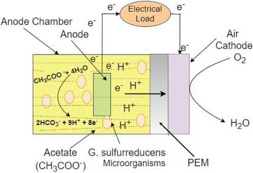
Ali Abul et al. (2016) created single-chamber microbial fuel cell model with a proton exchange membrane. Acetate is as the substrate and G. sulfurreducens is as the bacterium. Model presumptions can be found in Abul et al. (2016). The reactions in the anode and cathode parts are (1) $\begin{array}{rl}& \text{C}{\text{H}}_{\text{3}}\text{CO}{\text{O}}^{-}+\text{4}{\text{H}}_{\text{2}}\text{O}\to 2{\text{HCO}}_3^{-}+9{\text{H}}^{+}+8{\text{e}}^{-},\end{array}$(1) (2) $\begin{array}{rl}& {\text{O}}_2+4{\text{H}}^{+}+4{\text{e}}^{-}\to 2{\text{H}}_2\text{O}.\end{array}$(2)

2.1. MFC microbial kinetics

Monod balance gives the connection between dynamic biomass (the total amount of organism) and substrate dynamics. Dynamic biomass requires energy for maintenance which affected by the flow of electron and energy through endogenous decay. The net biomass development rate is the total of synthesis and decay rates, and is stated by (3) $\begin{array}{rl}\mu & ={\left(\frac{1}{X}\frac{dX}{dt}\right)}_{syn}+{\left(\frac{1}{X}\frac{dX}{dt}\right)}_{dec}={\mu }_{syn}+{\mu }_{dec}\\ & ={\mu }_{max}\frac{C_s}{k_s+C_s}-k_d,\end{array}$(3) where ${\mu }_{syn}$ and ${\mu }_{max}$ indicate specific growth rate and maximum specific growth rate of microorganisms respectively, $X$ shows the biomass concentration, $C_s$ specifies the substrate concentration, $k_s$ is the half saturation constant, $k_d>0$ is the decay coefficient. Bacteria break down the substrate and utilize it to live and grow. The cell growth is derived from the substrate utilization specified by (4) $q=q_{max}\frac{C_s}{K_s+C_s}$(4) where $q$ indicates the rate of substrate utilization and $q_{max}$ specifies the maximum rate of the same.

2.2. MFC physical model

MFC system gets a feed flow at the anode with a rate of $Q_a$ in terms of substrate concentration $C_{so}$ and regulates the MFC behaviour. The rate of change in substrate concentration and biomass concentration are respectively (5) $\begin{array}{rl}\frac{d{C}_s}{dt}& =-q^X+D(C_{so}-C_s),\\ \frac{dX}{dt}& =Y{q}_{max}\frac{C_s}{K_s+C_s}X-K_{d}X-DX,\end{array}$(5) where $D$ (the Dilution rate) states the control input and $Y$ specifies the growth yield (Abul et al., 2016). All typical values of single-population single-chamber MFC is given in Abul et al. (2016).

2.3. MFC controllable model

In this paper substrate concentration $C_s$, biomass concentration $X$ and dilution rate $D$ are considered as the states $x_1$, $x_2$ and input $u$ respectively. Substrate utilization and biomass growth are related by ${\mu }_{max}=Y.q_{max}$ and parameter ${\mu }_{max}$ is represented as $-{\theta }_1^{-1}$. The parametrized system dynamics are (6) $\begin{array}{rl}{\dot{x}}_1& =-{\theta }_1^{-1}.Y^{-1}\frac{x_1}{K_s+x_1}{x}_2+u(C_{so}-x_1)\\ {\dot{x}}_2& =\left({\theta }_1^{-1}\frac{x_1}{K_s+x_1}-K_d-u\right)x_2\end{array}$(6)

Values of $q_{max}$ and ${\mu }_{max}$ are $3d^{-1}$1 and $.4d^{-1}$ respectively (Abul et al., 2016). Maximum bacterial growth rate relies on the type of the organisms and limiting nutrients (Maier et al., 2009). The identifiable interval of the parameter ${\mu }_{max}$ is 3.01% with 95% confidence level (Pinto et al., 2010) and so $0.3699<{\theta }_1^{-1}<0.4301$.

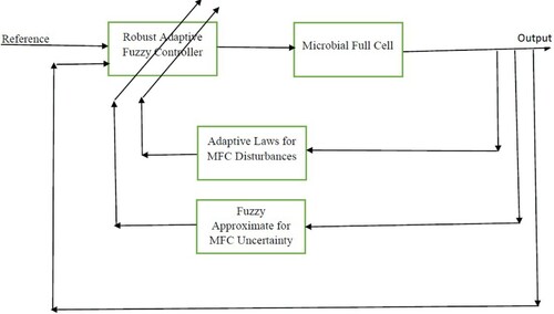
3. Fuzzy adaptive control

A block diagram of the MFC system with proposed controller is presented in Figure 2. With regard to external disturbances, the fuel cell system can be rewritten as follows. (7) $\begin{array}{rl}{\dot{x}}_1& =-{\theta }^{-1}{Y}^{-1}\frac{x_1}{k_s+x_1}{x}_2+u(c_{s0}-x_1)+d_1(t)\\ {\dot{x}}_2& =\left({\theta }^{-1}\frac{x_1}{k_s+x_1}-k_d-u\right)x_2+d_2(t)\end{array}$(7) where $d_1(t)$ and $d_2(t)$ are the bounded disturbances with unknown upper bounds. Let’s define the error as follows. (8) $\begin{array}{rl}{e}_1& =x_1-x_{1d}\\ e_2& =x_2-x_{2d}\end{array}$(8) where $x_{1d}$ and $x_{2d}$ are the desired equilibrium points. Error dynamics is obtained by deriving from the Equation (8) (9) $\begin{array}{rl}{\dot{e}}_1& =-{\theta }^{-1}{Y}^{-1}\frac{x_1{x}_2}{k_s+x_1}-x_{1}u+c_{s0}u\\ & +d_1(t)-{\dot{x}}_{1d}\\ {\dot{e}}_2& ={\theta }^{-1}\frac{x_1{x}_2}{k_s+x_1}-(x_2-1)u-k_d{e}_2-k_d{x}_{2d}\\ & -{\dot{x}}_{2d}-u_2+d_2(t)\end{array}$(9)

Figure 2. Block diagram of the MFC system with proposed controller.

By defining (10) $\begin{array}{rl}u& =u_1+u_2\\ {\psi }_1(.)& =-{\theta }^{-1}{Y}^{-1}\frac{x_1{x}_2}{k_s+x_1}-x_{1}u+c_{s0}{u}_2\\ {\psi }_2(.)& =-{\theta }^{-1}\frac{x_1{x}_2}{k_s+x_1}-(x_2-1)u-u_1\end{array}$(10)

The system error dynamics is rewritten as follows. (11) $\begin{array}{rl}{\dot{e}}_1& ={\psi }_1(.)+c_{s0}{u}_1-{\dot{x}}_{1d}+d_1(t)\\ {\dot{e}}_2& ={\psi }_2(.)-k_d{e}_2-k_d{x}_{2d}-{\dot{x}}_{2d}-u_2+d_2(t)\end{array}$(11)

To stabilize the error system, select the $u_1$ and $u_2$ control vectors as follows. (12) $\begin{array}{rl}{u}_1(t)& =\frac{1}{c_{s0}}({\dot{x}}_{1d}-k_1{e}_1-{\hat{\psi }}_1-{\hat{d}}_1)\\ u_2(t)& =-({\dot{x}}_{2d}+k_d{x}_{2d}-k_2{e}_2-{\hat{\psi }}_2-{\hat{d}}_2)\end{array}$(12) where ${\hat{d}}_1$ and ${\hat{d}}_2$ are adaptive estimators to eliminate the effect of disturbances. Also, ${\hat{\psi }}_1$ and ${\hat{\psi }}_2$ are approximators obtained from the fuzzy system to estimate the value of the functions ${{\psi }_1}_{(0)}$ and ${{\psi }_2}_{(0)}$ which are defined as follows. (13) $\begin{array}{r}{\hat{\psi }}_1={\hat{w}}_1^T{p}_1\\ {\hat{\psi }}_2={\hat{w}}_2^T{p}_2\end{array}$(13) ${\hat{w}}_1$ and ${\hat{w}}_2$ are estimates of fuzzy approximator weights. $p_1$ and $p_2$ are also fuzzy functions that use a 9-membership fuzzy rules system. (14) $p_i(x)=e^{-{(x-0.1i)}^2},i=1,2,\dots ,9$(14) To prove stability, Lyapunov function candidate is as follows: (15) $\begin{array}{rl}V(e_1,e_2)& =\frac{1}{2}{e}_1^2+\frac{1}{2}{e}_2^2+\frac{1}{2{\lambda }_1}{\tilde{w}}_1^T{\tilde{w}}_1\\ & +\frac{1}{2{\lambda }_2}{\tilde{w}}_2^T{\tilde{w}}_2+\frac{1}{2{\gamma }_1}{\tilde{d}}_1^2+\frac{1}{2{\gamma }_2}{\tilde{d}}_2^2\end{array}$(15) where $\begin{array}{rl}{\tilde{d}}_1& =d_1-{\hat{d}}_1\\ {\tilde{d}}_2& =d_2-{\hat{d}}_2\\ {\tilde{w}}_1& =w_1-{\hat{w}}_1\\ {\tilde{w}}_2& =w_2-{\hat{w}}_2\end{array}$ Deriving of Lyapunov function, it will be obtained. (16) $\begin{array}{rl}\dot{V}& =e_1{\dot{e}}_1+e_2{\dot{e}}_2-\frac{1}{{\lambda }_1}{\tilde{w}}_1^T{\dot{\hat{w}}}_1-\frac{1}{{\lambda }_2}{\tilde{w}}_2^T{\dot{\hat{w}}}_2-\frac{1}{{\gamma }_1}{\tilde{d}}_1{\dot{\hat{d}}}_1-\frac{1}{{\gamma }_2}{\tilde{d}}_2{\dot{\hat{d}}}_2\\ & =e_1({\psi }_1(.)+c_{s0}{u}_1-{\dot{x}}_{1d}+d_1(t))\\ & +e_2({\psi }_2(.)-k_d{e}_2-k_d{x}_{2d}-{\dot{x}}_{2d}\\ & -u_2+d_2(t))-\frac{1}{{\lambda }_1}{\tilde{w}}_1^T{\dot{\hat{w}}}_1\\ & -\frac{1}{{\lambda }_2}{\tilde{w}}_2^T{\dot{\hat{w}}}_2-\frac{1}{{\gamma }_1}{\tilde{d}}_1{\dot{\hat{d}}}_1-\frac{1}{{\gamma }_2}{\tilde{d}}_2{\dot{\hat{d}}}_2\end{array}$(16)

Now by placing $u_1$ and $u_2$ in the above equation we will have (17) $\begin{array}{rl}\dot{V}& =-k_1{e}_1^2-(k_d+k_2)e_2^2+e_1({\psi }_1(.)-{\hat{\psi }}_1+d_1(t)-{\hat{d}}_1)\\ & +e_2({\psi }_2(.)-{\hat{\psi }}_2+d_2(t)-{\hat{d}}_2)-\frac{1}{{\lambda }_1}{\tilde{w}}_1^T{\dot{\hat{w}}}_1-\frac{1}{{\lambda }_2}{\tilde{w}}_2^T{\dot{\hat{w}}}_2\\ & -\frac{1}{{\gamma }_1}{\tilde{d}}_1{\dot{\hat{d}}}_1-\frac{1}{{\gamma }_2}{\tilde{d}}_2{\dot{\hat{d}}}_2\end{array}$(17) By simplifying the above equation, it is obtained. (18) $\begin{array}{rl}\dot{V}& =-k_1{e}_1^2-(k_d+k_2)e_2^2+e_1{\tilde{w}}_1^T{p}_1+e_2{\tilde{w}}_2^T{p}_2\\ & +e_1{\tilde{d}}_1+e_2{\hat{d}}_2-\frac{1}{{\lambda }_1}{\tilde{w}}_1^T{\dot{\hat{w}}}_1\\ & -\frac{1}{{\lambda }_2}{\tilde{w}}_2^T{\dot{\hat{w}}}_2-\frac{1}{{\gamma }_1}{\tilde{d}}_1{\dot{\hat{d}}}_1-\frac{1}{{\gamma }_2}{\tilde{d}}_2{\dot{\hat{d}}}_2\end{array}$(18)

Now by defining the adaptive laws as following: (19) ${\dot{\hat{w}}}_1={\lambda }_1{e}_1{p}_1,{\dot{\hat{w}}}_2={\lambda }_2{e}_2{p}_2,{\dot{\hat{d}}}_1={\gamma }_1{e}_1,{\dot{\hat{d}}}_2={\gamma }_2{e}_2$(19) It is obtained. (20) $\dot{V}=-k_1{e}_1^2-(k_d+k_2)e_2^2\le 0$(20)

4. Simulation results

In this section, several scenarios for simulation are considered to show the capability of the proposed algorithm. The parameters used in the simulation for the model are in accordance with Patel and Deb (2018) and for the controller as follows. (21) $\begin{array}{rl}& k_1=0.01,k_2=0.2,{\lambda }_1=0.01,\\ & {\lambda }_2=0.01,{\gamma }_1=0.01,{\gamma }_2=0.01\end{array}$(21) To illustrate the effectiveness of the proposed method, a comparison is made between the system states and the states obtained from the adaptive backstepping method (Patel & Deb, 2018). We will now describe each of these scenarios.

Scenario 1

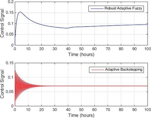
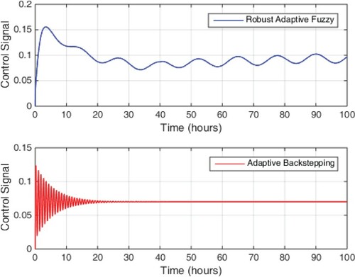
In this scenario, we assume that the model is completely accurate and that there is no uncertainty or disturbance. The results of the simulation are given in Figures 3–8. As can be seen from the figures, achieving the desired substrate concentration leading to a constant output voltage has been reached in the proposed method with less oscillation and less error. The proposed fuzzy adaptive controller is able to track the reference substrate concentration at a higher speed than the adaptive backstepping method. Anode and cathode voltages as well as MFC voltages were given in Figures 5–7, respectively. The control signal obtained from the proposed method and the adaptive backstepping method are shown in Figure 8. As can be seen from the figure, the obtained control signal has a positive value that ensures the physical realization of the obtained signal.

Figure 3. Performance of substrate concentration.

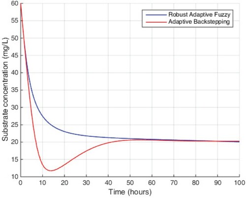
Figure 4. Performance of biomass concentration.

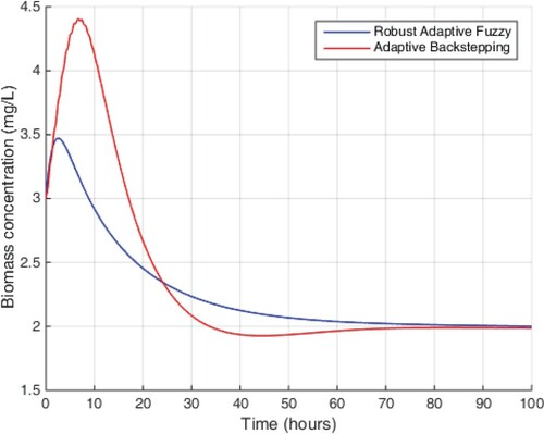
Figure 5. Anode voltages of single-chamber MFC.

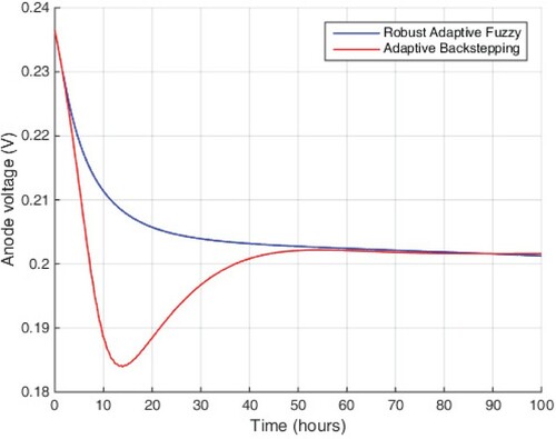
Figure 6. Cathode voltages of single-chamber MFC.

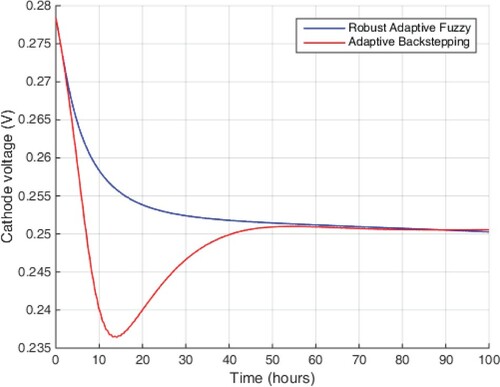
Figure 7. Voltages of single-chamber MFC.

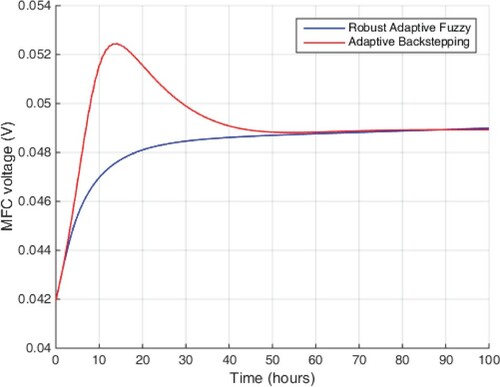
Figure 8. Control signal in scenario 1.

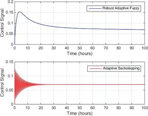
Figure 9. Performance of substrate concentration.

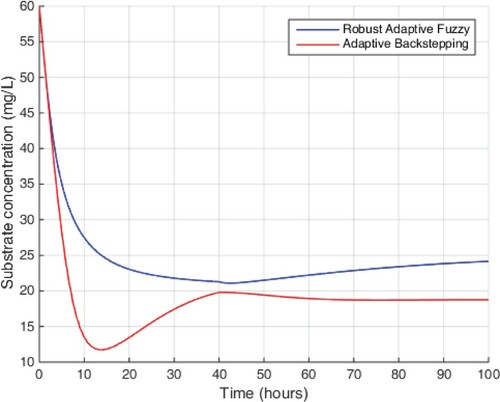
Figure 10. Performance of biomass concentration.

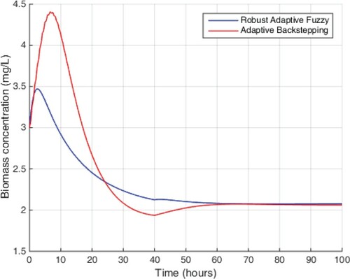
Figure 11. Anode voltages of single-chamber MFC.

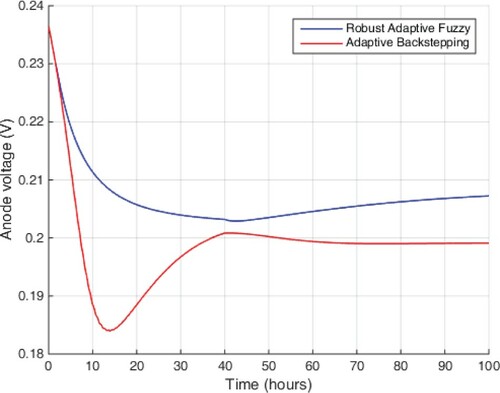
Figure 12. Cathode voltages of single-chamber MFC.

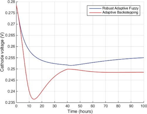
Figure 13. Voltages of single-chamber MFC.

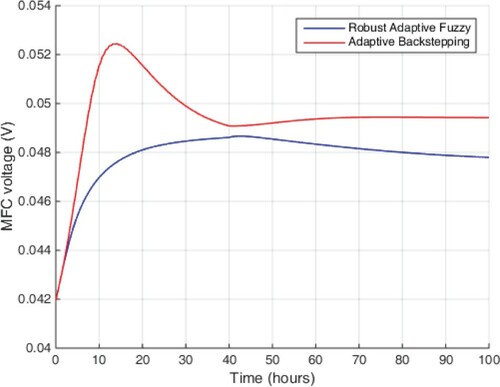
Figure 14. Control signal in scenario 2.

Scenario 2

In this scenario, the system has a parametric uncertainty in the following equation, but no external disturbance is considered. (22) $\{\begin{array}{cc}{\theta }^{-1}=0.4& \text{if }t<40\\ {\theta }^{-1}=0.42& \text{if }t\ge 40\end{array}$(22) Figures 9 and 10 show the system states under the proposed control method and the adaptive backstepping controller. As the previous scenario, using the proposed method, the desired substrate and biomass concentrations were achieved at higher speeds and with less error, while the adaptive backstepping method is not able to follow the target concentration due to disturbance. In other words, it is not able to reject uncertainty. Fuel cell output voltages are also shown in Figures 11–13. According to Figure 13, the optimal performance of the proposed method for maintaining the output voltage of MFC can be seen under the model uncertainty. The control signal obtained in this scenario is also shown in Figure 14.

Scenario 3

Figure 15. Performance of substrate concentration.

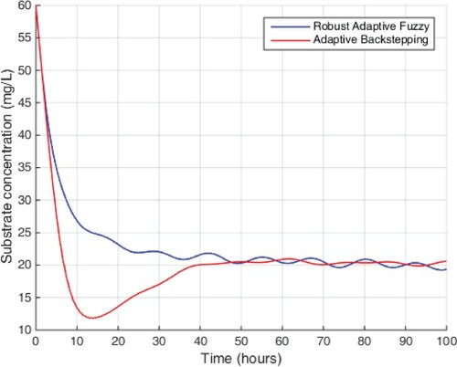
Figure 16. Performance of biomass concentration.

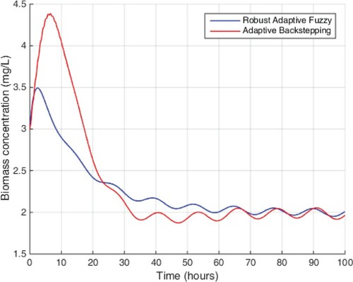
Figure 17. Anode voltages of single-chamber MFC.

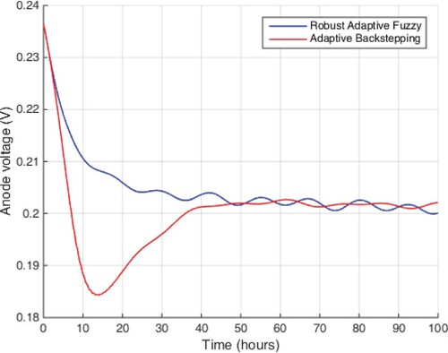
Figure 18. Cathode voltages of single-chamber MFC.

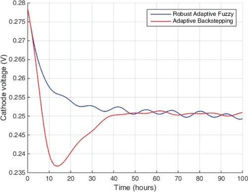
Figure 19. Voltages of single-chamber MFC.

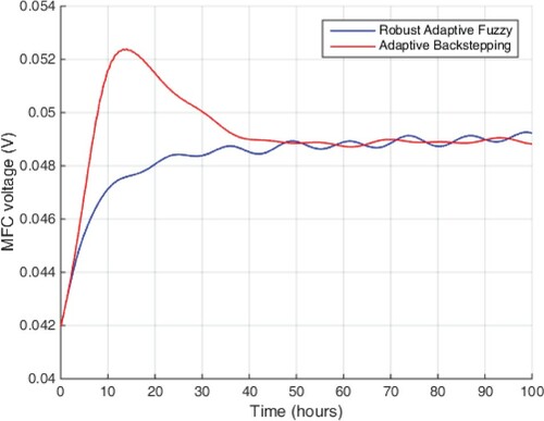
Figure 20. Control signal in scenario 3.

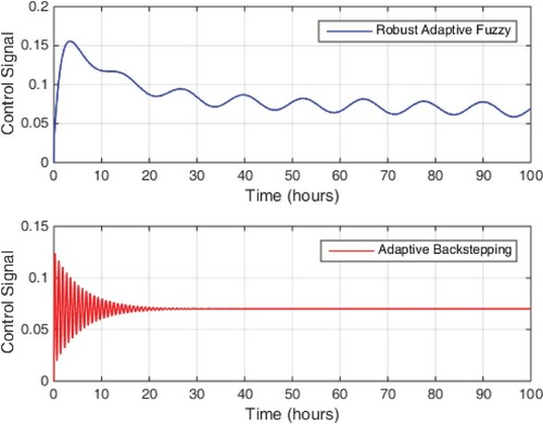
Figure 21. Performance of substrate concentration.

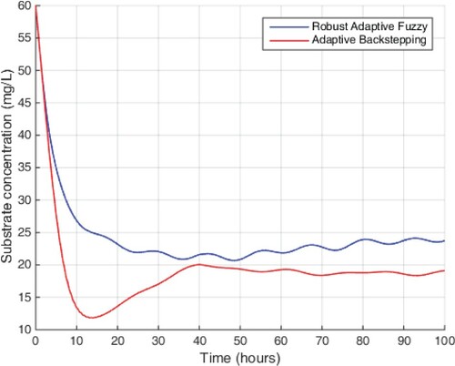
Figure 22. Performance of biomass concentration.

Figure 23. Anode voltages of single-chamber MFC.

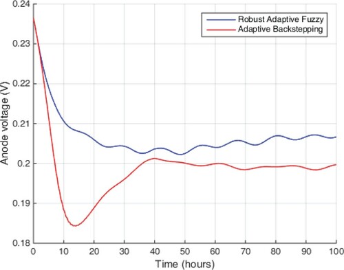
Figure 24. Cathode voltages of single-chamber MFC.

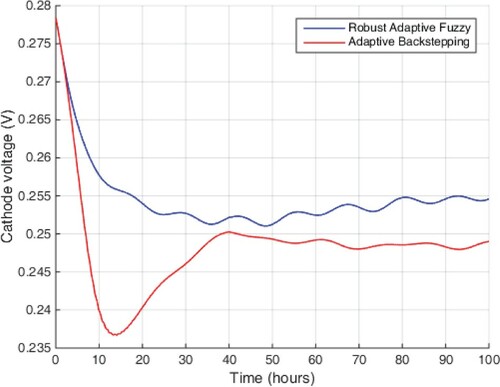
Figure 25. Voltages of single-chamber MFC.

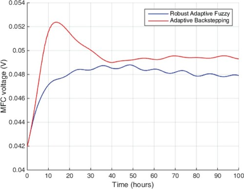
Figure 26. Control signal in scenario 4.

In this scenario, the MFC fuel cell system is disturbed, but the system parameters are not uncertain. The disturbance in the fuel cell system is considered as Eq. (23(23) $\begin{array}{rl}{d}_1(t)& =0.02\sin (0.3t)\\ d_2(t)& =0.03\cos (0.5t)\end{array}$(23) ), which can include all changes related to load, temperature, and substrate concentration. (23) $\begin{array}{rl}{d}_1(t)& =0.02\sin (0.3t)\\ d_2(t)& =0.03\cos (0.5t)\end{array}$(23) In this study, the disturbance upper bound is considered to be unknown but limited so that we can cover all of the above effects, even if we are not aware of the type of disturbance in the fuel cell system. The simulation results are shown in Figures 15–20. The ability of the proposed method to track the target concentration is well visible, whereas in this scenario, the adaptive backstepping method exhibits almost similar behaviour. The output voltage was also shown in Figures 17–19. From this scenario, the ability of the proposed method to reject disturbance and uncertainty is well visible. The control signal obtained in this scenario in Figure 20 shows that there is a possibility of physical realization of the control signal due to its positive.

Scenario 4

In this scenario, the uncertainty of the parameter is considered and the disturbance enters the system. The disturbance entered the system has all the descriptions and specifications of the disturbance introduced in the third scenario. The uncertainty of the parameter is similar to the second scenario. The simulation results in the presence of both uncertainty and disturbance are given in Figures 21–26. Like the second scenario, the adaptive backstepping controller is unable to track the target substrate concentration due to its inability to reject uncertainty, and therefore the output voltage of the MFC fluctuates and is non-functional, while the robust fuzzy adaptive method provided is able to track the desired concentration and deliver an output voltage with the least fluctuations despite the uncertainty of the parameter and disturbance. The control signal obtained in this scenario is also shown in Figure 26.

5. Conclusion

This paper presents a fuzzy adaptive control method for adjusting the substrate and biomass concentrations and finally the output voltage of single-chamber single-population microbial fuel cell. The purpose of the controller design is to achieve the desired output voltage in the presence of uncertainty, the effects of disturbance and nonlinear terms. The proposed controller is a combination of fuzzy and adaptive methods. The fuzzy method is used to approximate nonlinear terms and the parameter uncertainty effects, while the adaptive method plays two roles: The first role is to determine the weight of fuzzy approximators or fuzzy rules, and the next role is to overcome the effects of disturbances. From the simulation results, it is clear that the proposed method is successfully able to achieve the set goals and the robustness of the method was shown both in the proof and in the simulation.

Disclosure statement

No potential conflict of interest was reported by the author(s).

References

- Abul, A., Zhang, J., Steidl, R., Reguera, G., & Tan, X. (2016, July). Microbial fuel cells: Control-oriented modeling and experimental validation. In 2016 American Control Conference (ACC) (pp. 412–417). IEEE.
- Anaza, S. O., Abdulazeez, M. S., Yisah, Y. A., Yusuf, Y. O., Salawu, B. U., & Momoh, S. U. (2017). Micro hydro-electric energy generation – an overview. American Journal of Engineering Research (AJER), 6(2), 5–12.
- Atabani, A. E., Silitonga, A. S., Badruddin, I. A., Mahlia, T. M. I., Masjuki, H. H., & Mekhilef, S. (2012). A comprehensive review on biodiesel as an alternative energy resource and its characteristics. Renewable and Sustainable Energy Reviews, 16(4), 2070–2093. https://doi.org/https://doi.org/10.1016/j.rser.2012.01.003
- Boghani, H. C., Kim, J. R., Dinsdale, R. M., Guwy, A. J., & Premier, G. C. (2013). Control of power sourced from a microbial fuel cell reduces its start-up time and increases bioelectrochemical activity. Bioresource Technology, 140, 277–285. https://doi.org/https://doi.org/10.1016/j.biortech.2013.04.087
- Boghani, H. C., Michie, I., Dinsdale, R. M., Guwy, A. J., & Premier, G. C. (2016). Control of microbial fuel cell voltage using a gain scheduling control strategy. Journal of Power Sources, 322, 106–115. https://doi.org/https://doi.org/10.1016/j.jpowsour.2016.05.017
- Capuano, L. (2018). International energy outlook 2018 (IEO2018). US Energy Information Administration (EIA), 21.
- Chae, K. J., Choi, M. J., Lee, J. W., Kim, K. Y., & Kim, I. S. (2009). Effect of different substrates on the performance, bacterial diversity, and bacterial viability in microbial fuel cells. Bioresource Technology, 100(14), 3518–3525. https://doi.org/https://doi.org/10.1016/j.biortech.2009.02.065
- Chen, L., Bastin, G., & Van Breusegem, V. (1995). A case study of adaptive nonlinear regulation of fed-batch biological reactors. Automatica, 31(1), 55–65. https://doi.org/https://doi.org/10.1016/0005-1098(94)00068-T
- Cheng, J. (Ed.). (2017). Biomass to renewable energy processes. CRC Press.
- Choudhury, P., Uday, U. S. P., Mahata, N., Tiwari, O. N., Ray, R. N., Bandyopadhyay, T. K., & Bhunia, B. (2017). Performance improvement of microbial fuel cells for waste water treatment along with value addition: A review on past achievements and recent perspectives. Renewable and Sustainable Energy Reviews, 79, 372–389. https://doi.org/https://doi.org/10.1016/j.rser.2017.05.098
- Dochain, D. (1992). Adaptive control algorithms for nonminimum phase nonlinear bioreactors. Computers & Chemical Engineering, 16(5), 449–462. https://doi.org/https://doi.org/10.1016/0098-1354(92)85010-6
- Fan, L., Zhang, J., & Shi, X. (2015). Performance improvement of a microbial fuel cell based on model predictive control. International Journal of Electrochemical Science, 10(1), 737–748. 10.1.1.666.5279
- Fu, X., Fu, L., & Marrani, H. I. (2020). A Novel adaptive sliding mode control of microbial fuel cell in the presence of uncertainty. Journal of Electrical Engineering & Technology, 1–8. https://doi.org/https://doi.org/10.1007/s42835-020-00535-1
- Habermann, W., & Pommer, E. H. (1991). Biological fuel cells with sulphide storage capacity. Applied Microbiology and Biotechnology, 35(1), 128–133. https://doi.org/https://doi.org/10.1007/BF00180650
- Kannan, N., & Vakeesan, D. (2016). Solar energy for future world: A review. Renewable and Sustainable Energy Reviews, 62, 1092–1105. https://doi.org/https://doi.org/10.1016/j.rser.2016.05.022
- Lovley, D. R. (2006). Bug juice: Harvesting electricity with microorganisms. Nature Reviews Microbiology, 4(7), 497–508. https://doi.org/https://doi.org/10.1038/nrmicro1442
- Lovley, D. R. (2008). The microbe electric: Conversion of organic matter to electricity. Current Opinion in Biotechnology, 19(6), 564–571. https://doi.org/https://doi.org/10.1016/j.copbio.2008.10.005
- Maier, R. M., Pepper, I. L., & Gerba, C. P. (2009). Environmental microbiology (Vol. 397). Academic Press.
- Mamdani, E. H. (1974, December). Application of fuzzy algorithms for control of simple dynamic plant. In Proceedings of the Institution of Electrical Engineers (Vol. 121, No. 12, pp. 1585–1588). IET.
- Murthy, K. S. R., & Rahi, O. P. (2017). A comprehensive review of wind resource assessment. Renewable and Sustainable Energy Reviews, 72, 1320–1342. https://doi.org/https://doi.org/10.1016/j.rser.2016.10.038
- Newell, R. G., Qian, Y., & Raimi, D. (2016). Global energy outlook 2015 (No. w22075). National Bureau of Economic Research.
- Olasolo, P., Juárez, M. C., Morales, M. P., & Liarte, I. A. (2016). Enhanced geothermal systems (EGS): A review. Renewable and Sustainable Energy Reviews, 56, 133–144. https://doi.org/https://doi.org/10.1016/j.rser.2015.11.031
- Pant, D., Van Bogaert, G., Diels, L., & Vanbroekhoven, K. (2010). A review of the substrates used in microbial fuel cells (MFCs) for sustainable energy production. Bioresource Technology, 101(6), 1533–1543. https://doi.org/https://doi.org/10.1016/j.biortech.2009.10.017
- Patel, R., & Deb, D. (2018). Parametrized control-oriented mathematical model and adaptive backstepping control of a single chamber single population microbial fuel cell. Journal of Power Sources, 396, 599–605. https://doi.org/https://doi.org/10.1016/j.jpowsour.2018.06.064
- Pinto, R. P., Srinivasan, B., Manuel, M. F., & Tartakovsky, B. (2010). A two-population bio-electrochemical model of a microbial fuel cell. Bioresource Technology, 101(14), 5256–5265. https://doi.org/https://doi.org/10.1016/j.biortech.2010.01.122
- Slate, A. J., Whitehead, K. A., Brownson, D. A., & Banks, C. E. (2019). Microbial fuel cells: An overview of current technology. Renewable and Sustainable Energy Reviews, 101, 60–81. https://doi.org/https://doi.org/10.1016/j.rser.2018.09.044
- Sun, C., Shang, J., Luo, Z., Lu, Z., & Wang, R. (2018, July). A review of wave energy extraction technology. In IOP Conference Series: Materials Science and Engineering (Vol. 394, No. 4, p. 042038). IOP Publishing.
- Takagi, T., & Sugeno, M. (1985). Fuzzy identification of systems and its applications to modeling and control. IEEE Transactions on Systems, Man, and Cybernetics, (1), 116–132. https://doi.org/https://doi.org/10.1109/TSMC.1985.6313399
- Wilberforce, T., El Hassan, Z., Durrant, A., Thompson, J., Soudan, B., & Olabi, A. G. (2019). Overview of ocean power technology. Energy, 175, 165–181. https://doi.org/https://doi.org/10.1016/j.energy.2019.03.068
- Yan, M., & Fan, L. (2013). Constant voltage output in two-chamber microbial fuel cell under fuzzy PID control. International Journal of Electrochemical Science, 8, 3321–3332. 10.1.1.658.1933