State estimation via prediction-based scheme for linear time-varying uncertain networks with communication transmission delays and stochastic coupling

Abstract

In this paper, the design problem of recursive state estimation algorithm based on delay-prediction compensation is considered for a class of linear time-varying uncertain dynamical networks with network-induced communication transmission delays and stochastic coupling phenomenon. The random variables obeying Bernoulli distribution under uncertain occurrence probabilities are selected to depict the stochastic coupling phenomenon. Moreover, the modelling uncertainties and communication transmission delays are taken into account. Afterwards, a feasible prediction equation is constructed to compensate the communication transmission delays, and an updated time-varying state estimator is designed. Subsequently, the upper bound expression of the state estimation error covariance matrix is given by using the stochastic analysis technique and matrix theory, and the gain matrix of time-varying state estimator is obtained via minimizing the trace of such an upper bound. Furthermore, we present the mathematical proof which illustrates the monotonic relationship between the occurrence probabilities of stochastic coupling and the upper bound of error covariance. Finally, a simulation example is utilized to demonstrate the effectiveness of the proposed estimation strategy based on the delay prediction idea.

Keywords:

• Time-varying dynamical networks
• communication transmission delays
• stochastic coupling
• optimal estimation

1. Introduction

In recent years, the analysis methods of complex dynamical networks have played an important role in the big data transmissions, information processing and power grid (Baran & Rzysko, 2020; Bonello et al., 2020; Chen et al., 2019; Ding et al., 2019; Hernandez-torres et al., 2020; Wang et al., 2019). Recently, the networked control technology brings many conveniences to industrial development and technological advancements (Chen et al., 2020; Hu et al., 2017; Zou, Wang, Dong et al., 2020; Zou et al., 2019). However, the network-induced phenomena create new difficulties and challenges to the system analysis and design especially for the complex dynamical networks (Chen et al., 2019; Hu et al., 2016, 2020), where the complicated network couplings are generally involved among different nodes. On the other hand, due to the sudden changes of environmental conditions, the inherent features of sensors, the network faults and other reasons, it is inevitable that the information of node states can not be fully obtained (Hu, Wang, Liu, Jia et al., 2020; Zou, Wang, Hu et al., 2020). Therefore, it is of more important significance to design a scheme with higher accuracy for handling the state estimation problems (Wu et al., 2018; Xia et al., 2020; Xue et al., 2020; Zhao, 2018; Zhao & Mili, 2019). For example, some effective state estimation methods have been designed separately for time-varying dynamical systems as in Zhao (2018), Xia et al. (2020) and Xue et al. (2020), where the $H_{\mathrm{\infty }}$ performance constraint has been guaranteed and the feasibility of the proposed approaches has been illustrated. It is remarkable that the network topology is usually dynamically varying, such as uncertain coupling networks and time-varying stochastic coupling networks. To mention a few, Li and J. Du (2017) and Li et al. (2018) have described the coupling characteristics of different network nodes by employing the random variables obeying the uniform distribution. In addition, Liu et al. (2018) has discussed the coupling strengths by a coupling function, which is continuously once differentiable in variables. Nevertheless, we note that the investigation of the so-called stochastic coupling under uncertain occurrence probabilities as in Hu, Zhang, Kao et al. (2019) and Hu, Zhang, Yu et al. (2019) has not been deeply discussed.

In order to reflect the complexity of the actual dynamical system, there is a need to consider the parameter uncertainties due to the changes of internal structure and environmental impacts, which can not be ignored and estimated with difficulties (Luo et al., 2019). In order to facilitate the theoretical research from mathematics, the parameters uncertainties of the system model have been well discussed as in Bougofa et al. (2020) and Locke et al. (2020). Beyond that, Malinin and Gales (2018) has proposed a new framework for modelling the predictive uncertainties called Prior Networks, which can explicitly model the distributional uncertainties. It should be noticed that how to propose the effective analysis and syntheses - of schemes with strong robustness for dynamical systems is a key problem in control theory. In Ma et al. (2019), a distributed filtering method has been given for delayed uncertain nonlinear systems over sensor networks, in which the random perturbations have been modelled by the multiplicative noises and examined in detailed. Very recently, a new moving horizon state estimation method has been given in Zou, Wang, Hu et al. (2020), where both the unknown inputs as well as dynamic quantization impacts have been handled and the estimator parameters have been obtained based on the two-step design scheme including the decoupling and convergence step. Moreover, the stochastic uncertainty in the inner coupling term has been modelled in Hu, Wang, Liu, Jia et al. (2020) by utilizing the multiplicative noise, and a new state estimation strategy has been given based on the measurements transmitted through pre-defined event-triggered protocol.

As it is well known, the process of data transmission is unavoidable to be affected by many factors such as transmission speed, transmission mode and transmission environment, which induce that the data can not be received accurately in real time and the so-called communication transmission delays occur (Mao et al., 2021). It has been observed that the communication transmission delays should be considered in a proper way during the analysis of the dynamical systems, since it is well known that the delays can degrade the performance of the whole control system (Hu, Cui et al., 2020; Ma et al., 2018). Consequently, more attention has been paid to the control and estimation problem for dynamical systems with delays (An et al., 2018; Hu, Liu et al., 2020; Wu & He, 2017; Xiong et al., 2018) over the past decade. For instance, the effects of random sensor delays have been discussed in Hu, Liu et al. (2020) and a recursive estimation method applicable for time-varying dynamical networks with the online implementation advantages has been derived. However, it is worthwhile to point out that most of available state estimation approaches can be used in the time-invariant dynamical networks with time-delays only. Generally, it is noticed that the recursive state estimation problem has not been paid enough attention for the time-varying uncertain dynamical networks with communication transmission delays and stochastic coupling, not to mention the effort that active delay compensations are introduced.

In view of the above discussions, the main aim of paper is to design the prediction-based optimal estimation scheme, where both communication transmission delays and stochastic coupling are well discussed. When solving the addressed state estimation issue, the difficulties/challenges are listed from the following three aspects. (i) How to design a proper state estimator to attenuate the induced negative effects of communication transmission delays and stochastic coupling? In particular, a reasonable method is desired to examine the communication transmission delays. (ii) How to choose the desirable estimator gain matrix with easy-to-implement form and optimize the upper bound of estimation error covariance matrices? and (iii) How to evaluate the performance of proposed state estimation algorithm regarding the stochastic coupling from the theoretical viewpoint? To answer the mentioned three questions, the major contributions of this paper can be summarized as follows: (1) a new predictive updating strategy based on the delayed estimation information is presented to compensate the influences of communication transmission delays, which has a recursive characteristic; (2) a new prediction-based state estimator is constructed by fully taking the prediction-based estimation and statistical information of stochastic coupling; (3) the specific expression of the estimator gain is put forward by looking for a certain upper bound of the estimation error covariance in each step and minimizing such a obtained upper bound recursively; and (4) the monotonicity analysis is considered between the occurrence probabilities of stochastic coupling and the upper bound of error covariance matrix, where we provide the mathematical proof to demonstrate the inherent relationship by adding certain criteria. Finally, the effectiveness and feasibility of the prediction-based estimation scheme are verified by some simulations and comparisons presented in this paper, where we compare two categories including the cases with or without prediction method.

Notations: The symbols used throughout the paper are fairly standard. ${\mathbb{R}}^r$ depicts the r dimensional Euclidean space. I denotes the identity matrix of properly dimensions. For the matrix A and the vector x, $A^T$ and $x^T$ stand for the transposes of A and x, respectively. $\mathbb{E}\{x\}$ denotes the mathematical expectation of x. X>0 means that X is a positive-definite symmetric matrix. If not explicitly specified, these matrices are assumed to have compatible dimensions.

2. Problem formulation

Consider the following linear discrete time-varying networks with parameter uncertainties and stochastic coupling: (1) $\begin{array}{rl}{x}_{i,s+1}& =(A_{i,s}+\mathrm{\Delta }{A}_{i,s})x_{i,s}+c\sum _{j=1}^N{\alpha }_{ij,s}\mathrm{\Gamma }{x}_{j,s}\\ & +w_{i,s},i=1,2,\dots ,N,\end{array}$(1) (2) $\begin{array}{rl}{y}_{i,s}& =(C_{i,s}+\mathrm{\Delta }{C}_{i,s})x_{i,s}+v_{i,s},\end{array}$(2) where $x_{i,s}\in {\mathbb{R}}^n$ and $y_{i,s}\in {\mathbb{R}}^p$ represent the state of the ith node to be estimated and the measurement output of the ith node, respectively; the initial value of $x_{i,s}$ is $x_{i,0}$ with mean ${\overline{x}}_{i,0}$; c is a scalar that describes the overall coupling strength and Γ denotes a known inner-coupling matrix; $w_{i,s}\in {\mathbb{R}}^n$ and $v_{i,s}\in {\mathbb{R}}^p$ stand for the zero mean process noise with covariance $W_{i,s}>0$ and the zero mean measurement noise with covariance $V_{i,s}>0$, respectively; $\mathrm{\Delta }{A}_{i,s}=M_{i,s}{F}_{i,s}{H}_{i,s}$ and $\mathrm{\Delta }{C}_{i,s}={\mathcal{M}}_{i,s}{\mathcal{F}}_{i,s}{\mathcal{H}}_{i,s}$ depict the parameter uncertainties with $F_{i,s}{F}_{i,s}^T\le I$ and ${\mathcal{F}}_{i,s}{\mathcal{F}}_{i,s}^T\le I$. $A_{i,s}$, $C_{i,s}$, $M_{i,s}$, $H_{i,s}$, ${\mathcal{M}}_{i,s}$ and ${\mathcal{H}}_{i,s}$ are appropriately dimensional known matrices.

The phenomenon of stochastic coupling is modelled by a set of random variables ${\alpha }_{ij,s}$ $(i,j=1,2,\dots ,N)$ satisfying the Bernoulli distribution with (3) $\begin{array}{rl}\mathrm{Prob}\{{\alpha }_{ij,s}& =1\}=\mathbb{E}\{{\alpha }_{ij,s}\}={\beta }_{ij}+\mathrm{\Delta }{\beta }_{ij},\end{array}$(3) (4) $\begin{array}{rl}\mathrm{Prob}\{{\alpha }_{ij,s}& =0\}=1-\mathbb{E}\{{\alpha }_{ij,s}\}=1-({\beta }_{ij}+\mathrm{\Delta }{\beta }_{ij}),\end{array}$(4) where $({\beta }_{ij}+\mathrm{\Delta }{\beta }_{ij})\in [0,1]$, $|\mathrm{\Delta }{\beta }_{ij}|\le \epsilon$ with ε being a positive value. In the sequel, we make an assumption that ${\alpha }_{ij,s}$, $w_{i,s}$, $v_{i,s}$ and $x_{i,0}$ are mutually independent.

For the above mentioned linear time-varying uncertain stochastic networks, there is a need to provide an efficient state estimation method that is very appealing for the networks with a great number of nodes. However, it should be noted that the various transmission delays are inevitable among different network nodes during the communication. In other words, during the sharing of the state estimation information among the node i with the node j, there might be exist the communication transmission delays $d_{ij}$. Hence, in this paper, we introduce an active prediction method as follows: (5) $\begin{array}{rl}{\hat{x}}_{j,s-d_{ij}+1|s-d_{ij}}& =A_{j,s-d_{ij}}{\hat{x}}_{j,s-d_{ij}},\\ {\hat{x}}_{j,s-d_{ij}+2|s-d_{ij}}& =A_{j,s-d_{ij}+1}{\hat{x}}_{j,s-d_{ij}+1|s-d_{ij}},\\ & ⋮\\ {\hat{x}}_{j,s-1|s-d_{ij}}& =A_{j,s-2}{\hat{x}}_{j,s-2|s-d_{ij}},\\ {\hat{x}}_{j,s|s-d_{ij}}& =A_{j,s-1}{\hat{x}}_{j,s-1|s-d_{ij}}.\end{array}$(5) To facilitate the further developments, we set $A_{j,d_{ij}}=\prod _{l=1}^{d_{ij}}{A}_{j,s-l}$. Afterwards from (5(5) $\begin{array}{rl}{\hat{x}}_{j,s-d_{ij}+1|s-d_{ij}}& =A_{j,s-d_{ij}}{\hat{x}}_{j,s-d_{ij}},\\ {\hat{x}}_{j,s-d_{ij}+2|s-d_{ij}}& =A_{j,s-d_{ij}+1}{\hat{x}}_{j,s-d_{ij}+1|s-d_{ij}},\\ & ⋮\\ {\hat{x}}_{j,s-1|s-d_{ij}}& =A_{j,s-2}{\hat{x}}_{j,s-2|s-d_{ij}},\\ {\hat{x}}_{j,s|s-d_{ij}}& =A_{j,s-1}{\hat{x}}_{j,s-1|s-d_{ij}}.\end{array}$(5) ), it further implies that ${\hat{x}}_{j,s|s-d_{ij}}=A_{j,d_{ij}}{\hat{x}}_{j|s-d_{ij}}$. Then, for the ith node, we can introduce the following time-varying estimator based on the prediction estimation as in (5(5) $\begin{array}{rl}{\hat{x}}_{j,s-d_{ij}+1|s-d_{ij}}& =A_{j,s-d_{ij}}{\hat{x}}_{j,s-d_{ij}},\\ {\hat{x}}_{j,s-d_{ij}+2|s-d_{ij}}& =A_{j,s-d_{ij}+1}{\hat{x}}_{j,s-d_{ij}+1|s-d_{ij}},\\ & ⋮\\ {\hat{x}}_{j,s-1|s-d_{ij}}& =A_{j,s-2}{\hat{x}}_{j,s-2|s-d_{ij}},\\ {\hat{x}}_{j,s|s-d_{ij}}& =A_{j,s-1}{\hat{x}}_{j,s-1|s-d_{ij}}.\end{array}$(5) ): (6) $\begin{array}{rl}{\hat{x}}_{i,s+1}& =A_{i,s}{\hat{x}}_{i,s}+c{\beta }_{ii}\mathrm{\Gamma }{\hat{x}}_{i,s}+c\sum _{j=1,j\ne i}^N{\beta }_{ij}\mathrm{\Gamma }{\hat{x}}_{j,s\mid s-d_{ij}}\\ & +G_{i,s}(y_{i,s}-C_{i,s}{\hat{x}}_{i,s}),\end{array}$(6) where ${\hat{x}}_{i,s}$ represents the state estimation of $x_{i,s}$ at the moment s, and $G_{i,s}$ stands for the desirable estimator parameter matrix to be calculated later.

Remark 2.1

For the communication transmission delays, most of the existing estimation algorithms for complex dynamical networks have used the delay information directly when estimating the target state, which probably make the obtained results deviating from the real values significantly. For example, as mentioned in Hu, Liu et al. (2020), the sensor delays are discussed and the related estimation method is given based on the delay information. Moreover, it should be noticed that most of the existing estimation algorithms for complex dynamical networks with communication transmission delays can be applicable for the time-invariant system only. Consequently, there is urgent to propose an easy-to-implement estimation method with time-varying feature, which can actively compensate the communication transmission delays and effectively improve the estimation performance.

Remark 2.2

Unlike the existing estimation results, in order to ensure the estimation deviation as small as possible, both the state transition matrices of network nodes and the delayed estimation information are utilized to obtain the recursion equations by the predictive strategy (5(5) $\begin{array}{rl}{\hat{x}}_{j,s-d_{ij}+1|s-d_{ij}}& =A_{j,s-d_{ij}}{\hat{x}}_{j,s-d_{ij}},\\ {\hat{x}}_{j,s-d_{ij}+2|s-d_{ij}}& =A_{j,s-d_{ij}+1}{\hat{x}}_{j,s-d_{ij}+1|s-d_{ij}},\\ & ⋮\\ {\hat{x}}_{j,s-1|s-d_{ij}}& =A_{j,s-2}{\hat{x}}_{j,s-2|s-d_{ij}},\\ {\hat{x}}_{j,s|s-d_{ij}}& =A_{j,s-1}{\hat{x}}_{j,s-1|s-d_{ij}}.\end{array}$(5) ). It is worthwhile to mention that the state equations and state transition matrices are used to design the predictive strategy (5(5) $\begin{array}{rl}{\hat{x}}_{j,s-d_{ij}+1|s-d_{ij}}& =A_{j,s-d_{ij}}{\hat{x}}_{j,s-d_{ij}},\\ {\hat{x}}_{j,s-d_{ij}+2|s-d_{ij}}& =A_{j,s-d_{ij}+1}{\hat{x}}_{j,s-d_{ij}+1|s-d_{ij}},\\ & ⋮\\ {\hat{x}}_{j,s-1|s-d_{ij}}& =A_{j,s-2}{\hat{x}}_{j,s-2|s-d_{ij}},\\ {\hat{x}}_{j,s|s-d_{ij}}& =A_{j,s-1}{\hat{x}}_{j,s-1|s-d_{ij}}.\end{array}$(5) ), which can be seen as a certain compensation based on available information on handling the communication transmission delays and this method is fairly consistent with the traditionally predictive schemes. Accordingly, a new state estimator is constructed by fully employing the delay-prediction method, where the state estimation in the current instant k is obtained recursively by the utilizing the predictive strategy in (5(5) $\begin{array}{rl}{\hat{x}}_{j,s-d_{ij}+1|s-d_{ij}}& =A_{j,s-d_{ij}}{\hat{x}}_{j,s-d_{ij}},\\ {\hat{x}}_{j,s-d_{ij}+2|s-d_{ij}}& =A_{j,s-d_{ij}+1}{\hat{x}}_{j,s-d_{ij}+1|s-d_{ij}},\\ & ⋮\\ {\hat{x}}_{j,s-1|s-d_{ij}}& =A_{j,s-2}{\hat{x}}_{j,s-2|s-d_{ij}},\\ {\hat{x}}_{j,s|s-d_{ij}}& =A_{j,s-1}{\hat{x}}_{j,s-1|s-d_{ij}}.\end{array}$(5) ) and the estimation among different nodes are real-time updated and used when designing the state estimator (6(6) $\begin{array}{rl}{\hat{x}}_{i,s+1}& =A_{i,s}{\hat{x}}_{i,s}+c{\beta }_{ii}\mathrm{\Gamma }{\hat{x}}_{i,s}+c\sum _{j=1,j\ne i}^N{\beta }_{ij}\mathrm{\Gamma }{\hat{x}}_{j,s\mid s-d_{ij}}\\ & +G_{i,s}(y_{i,s}-C_{i,s}{\hat{x}}_{i,s}),\end{array}$(6) ). It should be noticed that the predictive idea is utilized and the corresponding information is explicitly reflected in the main results, which constitutes the major advantage of the predictive idea on handling the impacts of communication transmission delays. As it will be shown later, the predictive strategy in (5(5) $\begin{array}{rl}{\hat{x}}_{j,s-d_{ij}+1|s-d_{ij}}& =A_{j,s-d_{ij}}{\hat{x}}_{j,s-d_{ij}},\\ {\hat{x}}_{j,s-d_{ij}+2|s-d_{ij}}& =A_{j,s-d_{ij}+1}{\hat{x}}_{j,s-d_{ij}+1|s-d_{ij}},\\ & ⋮\\ {\hat{x}}_{j,s-1|s-d_{ij}}& =A_{j,s-2}{\hat{x}}_{j,s-2|s-d_{ij}},\\ {\hat{x}}_{j,s|s-d_{ij}}& =A_{j,s-1}{\hat{x}}_{j,s-1|s-d_{ij}}.\end{array}$(5) ) is useful on improving the estimation accuracy compared with the one employing the delayed estimation directly. In addition, the available probability information of stochastic coupling phenomenon is utilized when we design the state estimator, which can be seen additional effort to improve the estimation accuracy. After that, the major work is to deal with the caused influences from communication transmission delays and stochastic coupling phenomenon, moreover, a recursive estimation algorithm with online implementation feature is presented accordingly.

In the sequel, the estimation error and the estimation error covariance matrix are denoted by ${\tilde{x}}_{i,s+1}=x_{i,s+1}-{\hat{x}}_{i,s+1}$ and $Z_{i,s+1}=\mathbb{E}\{{\tilde{x}}_{i,s+1}{\tilde{x}}_{i,s+1}^T\}$, respectively. At present, the purposes of this paper are summarized as follows:

(P1)	For a class of time-varying uncertain networks with stochastic coupling and network-induced communication transmission delays, we design an optimal prediction-based robust estimation algorithm.
(P2)	Present the theoretical analysis on the monotonicity between the occurrence probabilities and the upper bound of the estimation error covariance matrix.

3. Design of state estimation strategy

In this section, based on the related definition, both the state covariance matrix and the state estimation error covariance matrix are calculated firstly. After that, the detailed expression of an optimal upper bound matrix of state estimation error covariance matrix is given and the state estimator gain is determined appropriately.

To start, we set ${\lambda }_{ij,s}={\alpha }_{ij,s}-{\beta }_{ij}-\mathrm{\Delta }{\beta }_{ij}$. Then, it can be seen that $\mathbb{E}\{{\lambda }_{ij,s}\}=0$ is obtained clearly. In view of (1(1) $\begin{array}{rl}{x}_{i,s+1}& =(A_{i,s}+\mathrm{\Delta }{A}_{i,s})x_{i,s}+c\sum _{j=1}^N{\alpha }_{ij,s}\mathrm{\Gamma }{x}_{j,s}\\ & +w_{i,s},i=1,2,\dots ,N,\end{array}$(1) ) and (6(6) $\begin{array}{rl}{\hat{x}}_{i,s+1}& =A_{i,s}{\hat{x}}_{i,s}+c{\beta }_{ii}\mathrm{\Gamma }{\hat{x}}_{i,s}+c\sum _{j=1,j\ne i}^N{\beta }_{ij}\mathrm{\Gamma }{\hat{x}}_{j,s\mid s-d_{ij}}\\ & +G_{i,s}(y_{i,s}-C_{i,s}{\hat{x}}_{i,s}),\end{array}$(6) ), one has (7) $\begin{array}{rl}{\tilde{x}}_{i,s+1}& =(A_{i,s}+c{\beta }_{ii}\mathrm{\Gamma }-G_{i,s}{C}_{i,s}){\tilde{x}}_{i,s}+c\sum _{j=1,j\ne i}^N{\beta }_{ij}\\ & \times \mathrm{\Gamma }(x_{j,s}-{\hat{x}}_{j,s|s-d_{ij}})+c\sum _{j=1}^N({\lambda }_{ij,s}+\mathrm{\Delta }{\beta }_{ij})\\ & \times \mathrm{\Gamma }{x}_{j,s}-G_{i,s}\mathrm{\Delta }{C}_{i,s}{x}_{i,s}+\mathrm{\Delta }{A}_{i,s}{x}_{i,s}\\ & -G_{i,s}{v}_{i,s}+w_{i,s}.\end{array}$(7) To proceed, three theorems are proposed which include the specific expressions of an optimal upper bound of state covariance matrix, state estimation error covariance matrix and an optimal upper bound of state estimation error covariance matrix.

Theorem 3.1

Consider the time-varying uncertain dynamical networks (1(1) $\begin{array}{rl}{x}_{i,s+1}& =(A_{i,s}+\mathrm{\Delta }{A}_{i,s})x_{i,s}+c\sum _{j=1}^N{\alpha }_{ij,s}\mathrm{\Gamma }{x}_{j,s}\\ & +w_{i,s},i=1,2,\dots ,N,\end{array}$(1) )–(2(2) $\begin{array}{rl}{y}_{i,s}& =(C_{i,s}+\mathrm{\Delta }{C}_{i,s})x_{i,s}+v_{i,s},\end{array}$(2) ) with the state estimator (6(6) $\begin{array}{rl}{\hat{x}}_{i,s+1}& =A_{i,s}{\hat{x}}_{i,s}+c{\beta }_{ii}\mathrm{\Gamma }{\hat{x}}_{i,s}+c\sum _{j=1,j\ne i}^N{\beta }_{ij}\mathrm{\Gamma }{\hat{x}}_{j,s\mid s-d_{ij}}\\ & +G_{i,s}(y_{i,s}-C_{i,s}{\hat{x}}_{i,s}),\end{array}$(6) ). Under the initial conditions ${\mathcal{X}}_{i,0}=X_{i,0}$, an optimal upper bound ${\mathcal{X}}_{i,s+1}$ of state covariance matrix $X_{i,s+1}$ can be given as below: (8) $\begin{array}{rl}{\mathcal{X}}_{i,s+1}& =(1+{\mu }_1+{\mu }_2)A_{i,s}{\mathcal{X}}_{i,s}{A}_{i,s}^T+(1+{\mu }_1^{-1}+{\mu }_3)\\ & \times \mathrm{tr}(H_{i,s}{\mathcal{X}}_{i,s}{H}_{i,s}^T)M_{i,s}{M}_{i,s}^T+(1+{\mu }_2^{-1}+{\mu }_3^{-1})\\ & \times c^{2}N\sum _{j=1}^N({\beta }_{ij}+\epsilon )\mathrm{\Gamma }{\mathcal{X}}_{j,s}{\mathrm{\Gamma }}^T+W_{i,s},\end{array}$(8) where ${\mu }_t>0(t=1,2,3)$ are scalars.

Proof.

Considering the time-varying uncertain dynamical networks (1(1) $\begin{array}{rl}{x}_{i,s+1}& =(A_{i,s}+\mathrm{\Delta }{A}_{i,s})x_{i,s}+c\sum _{j=1}^N{\alpha }_{ij,s}\mathrm{\Gamma }{x}_{j,s}\\ & +w_{i,s},i=1,2,\dots ,N,\end{array}$(1) ), one has: (9) $\begin{array}{rl}{X}_{i,s+1}& =\mathbb{E}\left\{x_{i,s+1}{x}_{i,s+1}^T\right\}\\ & =A_{i,s}{X}_{i,s}{A}_{i,s}^T+M_{i,s}{F}_{i,s}{H}_{i,s}{X}_{i,s}{H}_{i,s}^T{F}_{i,s}^T{M}_{i,s}^T\\ & +c^2\mathbb{E}\left\{\left[\sum _{j=1}^N{\alpha }_{ij,s}\mathrm{\Gamma }{x}_{j,s}\right]{\left[\sum _{j=1}^N{\alpha }_{ij,s}\mathrm{\Gamma }{x}_{j,s}\right]}^T\right\}\\ & +{\mathcal{B}}_{1,s}+{\mathcal{B}}_{1,s}^T+{\mathcal{B}}_{2,s}+{\mathcal{B}}_{2,s}^T+{\mathcal{B}}_{3,s}+{\mathcal{B}}_{3,s}^T+{\mathcal{B}}_{4,s}\\ & +{\mathcal{B}}_{4,s}^T+{\mathcal{B}}_{5,s}+{\mathcal{B}}_{5,s}^T+{\mathcal{B}}_{6,s}+{\mathcal{B}}_{6,s}^T+W_{i,s},\end{array}$(9) where $\begin{array}{rl}{\mathcal{B}}_{1,s}& =A_{i,s}\mathbb{E}\left\{x_{i,s}{x}_{i,s}^T\right\}{H}_{i,s}^T{F}_{i,s}^T{M}_{i,s}^T,\\ {\mathcal{B}}_{2,s}& =c{A}_{i,s}\mathbb{E}\left\{x_{i,s}{\left[\sum _{j=1}^N{\alpha }_{ij,s}\mathrm{\Gamma }{x}_{j,s}\right]}^T\right\},\\ {\mathcal{B}}_{3,s}& =c\mathbb{E}\left\{\left[\sum _{j=1}^N{\alpha }_{ij,s}\mathrm{\Gamma }{x}_{j,s}\right]x_{i,s}^T\right\}{H}_{i,s}^T{F}_{i,s}^T{M}_{i,s}^T,\\ {\mathcal{B}}_{4,s}& =A_{i,s}\mathbb{E}\left\{x_{i,s}{w}_{i,s}^T\right\},\\ {\mathcal{B}}_{5,s}& =M_{i,s}{F}_{i,s}{H}_{i,s}\mathbb{E}\left\{x_{i,s}{w}_{i,s}^T\right\},\\ {\mathcal{B}}_{6,s}& =c\mathbb{E}\left\{\left[\sum _{j=1}^N{\alpha }_{ij,s}\mathrm{\Gamma }{x}_{j,s}\right]w_{i,s}^T\right\}.\end{array}$Since $w_{i,s}$ is zero mean noise, then we conclude that ${\mathcal{B}}_{t,s}=0(t=4,5,6)$. After that, for any two vectors $x,y\in {\mathbb{R}}^n$, using the inequality $x{y}^T+y{x}^T\le \delta x{x}^T+{\delta }^{-1}y{y}^T$, where $\delta >0$ is a constant scalar, the crossed and unknown terms in (9(9) $\begin{array}{rl}{X}_{i,s+1}& =\mathbb{E}\left\{x_{i,s+1}{x}_{i,s+1}^T\right\}\\ & =A_{i,s}{X}_{i,s}{A}_{i,s}^T+M_{i,s}{F}_{i,s}{H}_{i,s}{X}_{i,s}{H}_{i,s}^T{F}_{i,s}^T{M}_{i,s}^T\\ & +c^2\mathbb{E}\left\{\left[\sum _{j=1}^N{\alpha }_{ij,s}\mathrm{\Gamma }{x}_{j,s}\right]{\left[\sum _{j=1}^N{\alpha }_{ij,s}\mathrm{\Gamma }{x}_{j,s}\right]}^T\right\}\\ & +{\mathcal{B}}_{1,s}+{\mathcal{B}}_{1,s}^T+{\mathcal{B}}_{2,s}+{\mathcal{B}}_{2,s}^T+{\mathcal{B}}_{3,s}+{\mathcal{B}}_{3,s}^T+{\mathcal{B}}_{4,s}\\ & +{\mathcal{B}}_{4,s}^T+{\mathcal{B}}_{5,s}+{\mathcal{B}}_{5,s}^T+{\mathcal{B}}_{6,s}+{\mathcal{B}}_{6,s}^T+W_{i,s},\end{array}$(9) ) are handled as $\begin{array}{rl}{\mathcal{B}}_{1,s}+{\mathcal{B}}_{1,s}^T& \le {\mu }_1{A}_{i,s}{X}_{i,s}{A}_{i,s}^T\\ & +{\mu }_1^{-1}{M}_{i,s}{F}_{i,s}{H}_{i,s}{X}_{i,s}{H}_{i,s}^T{F}_{i,s}^T{M}_{i,s}^T,\\ {\mathcal{B}}_{2,s}+{\mathcal{B}}_{2,s}^T& \le {\mu }_2{A}_{i,s}{X}_{i,s}{A}_{i,s}^T+{\mu }_2^{-1}{c}^2\\ & \times \mathbb{E}\left\{\left[\sum _{j=1}^N{\alpha }_{ij,s}\mathrm{\Gamma }{x}_{j,s}\right]{\left[\sum _{j=1}^N{\alpha }_{ij,s}\mathrm{\Gamma }{x}_{j,s}\right]}^T\right\},\\ {\mathcal{B}}_{3,s}+{\mathcal{B}}_{3,s}^T& \le {\mu }_3{M}_{i,s}{F}_{i,s}{H}_{i,s}{X}_{i,s}{H}_{i,s}^T{F}_{i,s}^T{M}_{i,s}^T+{\mu }_3^{-1}{c}^2\\ & \times \mathbb{E}\left\{\left[\sum _{j=1}^N{\alpha }_{ij,s}\mathrm{\Gamma }{x}_{j,s}\right]{\left[\sum _{j=1}^N{\alpha }_{ij,s}\mathrm{\Gamma }{x}_{j,s}\right]}^T\right\},\end{array}$where ${\mu }_t>0(t=1,2,3)$ are scalars. Then, it follows from above that (9(9) $\begin{array}{rl}{X}_{i,s+1}& =\mathbb{E}\left\{x_{i,s+1}{x}_{i,s+1}^T\right\}\\ & =A_{i,s}{X}_{i,s}{A}_{i,s}^T+M_{i,s}{F}_{i,s}{H}_{i,s}{X}_{i,s}{H}_{i,s}^T{F}_{i,s}^T{M}_{i,s}^T\\ & +c^2\mathbb{E}\left\{\left[\sum _{j=1}^N{\alpha }_{ij,s}\mathrm{\Gamma }{x}_{j,s}\right]{\left[\sum _{j=1}^N{\alpha }_{ij,s}\mathrm{\Gamma }{x}_{j,s}\right]}^T\right\}\\ & +{\mathcal{B}}_{1,s}+{\mathcal{B}}_{1,s}^T+{\mathcal{B}}_{2,s}+{\mathcal{B}}_{2,s}^T+{\mathcal{B}}_{3,s}+{\mathcal{B}}_{3,s}^T+{\mathcal{B}}_{4,s}\\ & +{\mathcal{B}}_{4,s}^T+{\mathcal{B}}_{5,s}+{\mathcal{B}}_{5,s}^T+{\mathcal{B}}_{6,s}+{\mathcal{B}}_{6,s}^T+W_{i,s},\end{array}$(9) ) can be expressed as (10) $\begin{array}{rl}{X}_{i,s+1}& \le (1+{\mu }_1+{\mu }_2)A_{i,s}{X}_{i,s}{A}_{i,s}^T+(1+{\mu }_1^{-1}+{\mu }_3)\\ & \times M_{i,s}{F}_{i,s}{H}_{i,s}{X}_{i,s}{H}_{i,s}^T{F}_{i,s}^T{M}_{i,s}^T\\ & +(1+{\mu }_2^{-1}+{\mu }_3^{-1})c^2\mathbb{E}\{\left[\sum _{j=1}^N{\alpha }_{ij,s}\mathrm{\Gamma }{x}_{j,s}\right]\\ & \times {\left[\sum _{j=1}^N{\alpha }_{ij,s}\mathrm{\Gamma }{x}_{j,s}\right]}^T\}+W_{i,s}.\end{array}$(10) Next, the second term in (10(10) $\begin{array}{rl}{X}_{i,s+1}& \le (1+{\mu }_1+{\mu }_2)A_{i,s}{X}_{i,s}{A}_{i,s}^T+(1+{\mu }_1^{-1}+{\mu }_3)\\ & \times M_{i,s}{F}_{i,s}{H}_{i,s}{X}_{i,s}{H}_{i,s}^T{F}_{i,s}^T{M}_{i,s}^T\\ & +(1+{\mu }_2^{-1}+{\mu }_3^{-1})c^2\mathbb{E}\{\left[\sum _{j=1}^N{\alpha }_{ij,s}\mathrm{\Gamma }{x}_{j,s}\right]\\ & \times {\left[\sum _{j=1}^N{\alpha }_{ij,s}\mathrm{\Gamma }{x}_{j,s}\right]}^T\}+W_{i,s}.\end{array}$(10) ) is tackled as (11) $\begin{array}{rl}& M_{i,s}{F}_{i,s}{H}_{i,s}{X}_{i,s}{H}_{i,s}^T{F}_{i,s}^T{M}_{i,s}^T\\ & \le \mathrm{tr}\left(H_{i,s}{X}_{i,s}{H}_{i,s}^T\right)M_{i,s}{M}_{i,s}^T.\end{array}$(11) Moreover, the third term in (10(10) $\begin{array}{rl}{X}_{i,s+1}& \le (1+{\mu }_1+{\mu }_2)A_{i,s}{X}_{i,s}{A}_{i,s}^T+(1+{\mu }_1^{-1}+{\mu }_3)\\ & \times M_{i,s}{F}_{i,s}{H}_{i,s}{X}_{i,s}{H}_{i,s}^T{F}_{i,s}^T{M}_{i,s}^T\\ & +(1+{\mu }_2^{-1}+{\mu }_3^{-1})c^2\mathbb{E}\{\left[\sum _{j=1}^N{\alpha }_{ij,s}\mathrm{\Gamma }{x}_{j,s}\right]\\ & \times {\left[\sum _{j=1}^N{\alpha }_{ij,s}\mathrm{\Gamma }{x}_{j,s}\right]}^T\}+W_{i,s}.\end{array}$(10) ) is handled as (12) $\begin{array}{rl}& \mathbb{E}\left\{\left[\sum _{j=1}^N{\alpha }_{ij,s}\mathrm{\Gamma }{x}_{j,s}\right]{\left[\sum _{j=1}^N{\alpha }_{ij,s}\mathrm{\Gamma }{x}_{j,s}\right]}^T\right\}\\ & \le N\sum _{j=1}^N({\beta }_{ij}+\epsilon )\mathrm{\Gamma }{X}_{j,s}{\mathrm{\Gamma }}^T.\end{array}$(12) Finally, together with (10(10) $\begin{array}{rl}{X}_{i,s+1}& \le (1+{\mu }_1+{\mu }_2)A_{i,s}{X}_{i,s}{A}_{i,s}^T+(1+{\mu }_1^{-1}+{\mu }_3)\\ & \times M_{i,s}{F}_{i,s}{H}_{i,s}{X}_{i,s}{H}_{i,s}^T{F}_{i,s}^T{M}_{i,s}^T\\ & +(1+{\mu }_2^{-1}+{\mu }_3^{-1})c^2\mathbb{E}\{\left[\sum _{j=1}^N{\alpha }_{ij,s}\mathrm{\Gamma }{x}_{j,s}\right]\\ & \times {\left[\sum _{j=1}^N{\alpha }_{ij,s}\mathrm{\Gamma }{x}_{j,s}\right]}^T\}+W_{i,s}.\end{array}$(10) )–(12(12) $\begin{array}{rl}& \mathbb{E}\left\{\left[\sum _{j=1}^N{\alpha }_{ij,s}\mathrm{\Gamma }{x}_{j,s}\right]{\left[\sum _{j=1}^N{\alpha }_{ij,s}\mathrm{\Gamma }{x}_{j,s}\right]}^T\right\}\\ & \le N\sum _{j=1}^N({\beta }_{ij}+\epsilon )\mathrm{\Gamma }{X}_{j,s}{\mathrm{\Gamma }}^T.\end{array}$(12) ), we can get (13) $\begin{array}{rl}{X}_{i,s+1}& leq(1+{\mu }_1+{\mu }_2)A_{i,s}{X}_{i,s}{A}_{i,s}^T+(1+{\mu }_1^{-1}+{\mu }_3)\\ & \times \mathrm{tr}\left(H_{i,s}{X}_{i,s}{H}_{i,s}^T\right)M_{i,s}{M}_{i,s}^T+(1+{\mu }_2^{-1}+{\mu }_3^{-1})\\ & \times c^{2}N\sum _{j=1}^N({\beta }_{ij}+\epsilon )\mathrm{\Gamma }{X}_{j,s}{\mathrm{\Gamma }}^T+W_{i,s}.\end{array}$(13) According to the initial conditions, it is easy to gain that $X_{i,s+1}\le {\mathcal{X}}_{i,s+1}$, where ${\mathcal{X}}_{i,s+1}$ is defined in (8(8) $\begin{array}{rl}{\mathcal{X}}_{i,s+1}& =(1+{\mu }_1+{\mu }_2)A_{i,s}{\mathcal{X}}_{i,s}{A}_{i,s}^T+(1+{\mu }_1^{-1}+{\mu }_3)\\ & \times \mathrm{tr}(H_{i,s}{\mathcal{X}}_{i,s}{H}_{i,s}^T)M_{i,s}{M}_{i,s}^T+(1+{\mu }_2^{-1}+{\mu }_3^{-1})\\ & \times c^{2}N\sum _{j=1}^N({\beta }_{ij}+\epsilon )\mathrm{\Gamma }{\mathcal{X}}_{j,s}{\mathrm{\Gamma }}^T+W_{i,s},\end{array}$(8) ). In summary, the proof is complete.

Theorem 3.2

Considering the time-varying uncertain dynamical networks (1(1) $\begin{array}{rl}{x}_{i,s+1}& =(A_{i,s}+\mathrm{\Delta }{A}_{i,s})x_{i,s}+c\sum _{j=1}^N{\alpha }_{ij,s}\mathrm{\Gamma }{x}_{j,s}\\ & +w_{i,s},i=1,2,\dots ,N,\end{array}$(1) )–(2(2) $\begin{array}{rl}{y}_{i,s}& =(C_{i,s}+\mathrm{\Delta }{C}_{i,s})x_{i,s}+v_{i,s},\end{array}$(2) ) with the state estimator in (6(6) $\begin{array}{rl}{\hat{x}}_{i,s+1}& =A_{i,s}{\hat{x}}_{i,s}+c{\beta }_{ii}\mathrm{\Gamma }{\hat{x}}_{i,s}+c\sum _{j=1,j\ne i}^N{\beta }_{ij}\mathrm{\Gamma }{\hat{x}}_{j,s\mid s-d_{ij}}\\ & +G_{i,s}(y_{i,s}-C_{i,s}{\hat{x}}_{i,s}),\end{array}$(6) ), the recursive equation of state estimation error covariance matrix $Z_{i,s+1}$ can be proposed as: (14) $\begin{array}{rl}{Z}_{i,s+1}& =(A_{i,s}+c{\beta }_{ii}\mathrm{\Gamma }-G_{i,s}{C}_{i,s})Z_{i,s}\\ & \times {(A_{i,s}+c{\beta }_{ii}\mathrm{\Gamma }-G_{i,s}{C}_{i,s})}^T\\ & +c^2\mathbb{E}\{\left[\sum _{j=1,j\ne i}^N{\beta }_{ij}\mathrm{\Gamma }(x_{j,s}-{\hat{x}}_{j,s\mid s-d_{ij}})\right]\\ & \times {\left[\sum _{j=1,j\ne i}^N{\beta }_{ij}\mathrm{\Gamma }(x_{j,s}-{\hat{x}}_{j,s\mid s-d_{ij}})\right]}^T\}\\ & +c^2\mathbb{E}\left\{\left[\sum _{j=1}^N{\lambda }_{ij,s}\mathrm{\Gamma }{x}_{j,s}\right]{\left[\sum _{j=1}^N{\lambda }_{ij,s}\mathrm{\Gamma }{x}_{j,s}\right]}^T\right\}\\ & +c^2\mathbb{E}\left\{\left[\sum _{j=1}^N\mathrm{\Delta }{\beta }_{ij}\mathrm{\Gamma }{x}_{j,s}\right]{\left[\sum _{j=1}^N\mathrm{\Delta }{\beta }_{ij}\mathrm{\Gamma }{x}_{j,s}\right]}^T\right\}\\ & +\mathrm{\Delta }{A}_{i,s}{X}_{i,s}{A}_{i,s}^T+G_{i,s}\mathrm{\Delta }{C}_{i,s}{X}_{i,s}\mathrm{\Delta }{C}_{i,s}^T{G}_{i,s}^T\\ & +{\mathcal{D}}_{1,s}+{\mathcal{D}}_{1,s}^T+{\mathcal{D}}_{2,s}+{\mathcal{D}}_{2,s}^T+{\mathcal{D}}_{3,s}+{\mathcal{D}}_{3,s}^T\\ & +{\mathcal{D}}_{4,s}+{\mathcal{D}}_{4,s}^T+{\mathcal{D}}_{5,s}+{\mathcal{D}}_{5,s}^T+{\mathcal{D}}_{6,s}+{\mathcal{D}}_{6,s}^T\\ & +{\mathcal{D}}_{7,s}+{\mathcal{D}}_{7,s}^T+{\mathcal{D}}_{8,s}+{\mathcal{D}}_{8,s}^T+{\mathcal{D}}_{9,s}+{\mathcal{D}}_{9,s}^T\\ & +{\mathcal{D}}_{10,s}+{\mathcal{D}}_{10,s}^T+G_{i,s}{V}_{i,s}{G}_{i,s}^T+W_{i,s},\end{array}$(14) where $\begin{array}{rl}{\mathcal{D}}_{1,s}& =c(A_{i,s}+c{\beta }_{ii}\mathrm{\Gamma }-G_{i,s}{C}_{i,s})\\ & \times \mathbb{E}\left\{{\tilde{x}}_{i,s}{\left[\sum _{j=1,j\ne i}^N{\beta }_{ij}\mathrm{\Gamma }(x_{j,s}-{\hat{x}}_{j,s\mid s-d_{ij}})\right]}^T\right\},\\ {\mathcal{D}}_{2,s}& =c(A_{i,s}+c{\beta }_{ii}\mathrm{\Gamma }-G_{i,s}{C}_{i,s})\\ & \times \mathbb{E}\left\{{\tilde{x}}_{i,s}{\left[\sum _{j=1}^N\mathrm{\Delta }{\beta }_{ij}\mathrm{\Gamma }{x}_{j,s}\right]}^T\right\},\\ {\mathcal{D}}_{3,s}& =-(A_{i,s}+c{\beta }_{ii}\mathrm{\Gamma }-G_{i,s}{C}_{i,s})\mathbb{E}\left\{{\tilde{x}}_{i,s}{x}_{i,s}^T\right\}\mathrm{\Delta }{C}_{i,s}^T{G}_{i,s}^T,\\ {\mathcal{D}}_{4,s}& =(A_{i,s}+c{\beta }_{ii}\mathrm{\Gamma }-G_{i,s}{C}_{i,s})\mathbb{E}\left\{{\tilde{x}}_{i,s}{x}_{i,s}^T\right\}\mathrm{\Delta }{A}_{i,s}^T,\\ {\mathcal{D}}_{5,s}& =c^2\mathbb{E}\{\left[\sum _{j=1,j\ne i}^N{\beta }_{ij}\mathrm{\Gamma }(x_{j,s}-{\hat{x}}_{j,s\mid s-d_{ij}})\right]\\ & \times {\left[\sum _{j=1}^N\mathrm{\Delta }{\beta }_{ij}\mathrm{\Gamma }{x}_{j,s}\right]}^T\},\\ {\mathcal{D}}_{6,s}& =-c\mathbb{E}\left\{\left[\sum _{j=1,j\ne i}^N{\beta }_{ij}\mathrm{\Gamma }(x_{j,s}-{\hat{x}}_{j,s\mid s-d_{ij}})\right]x_{i,s}^T\right\}\\ & \times \mathrm{\Delta }{C}_{i,s}^T{G}_{i,s}^T,{\mathcal{D}}_{7,s}\\ & =c\mathbb{E}\left\{\left[\sum _{j=1,j\ne i}^N{\beta }_{ij}\mathrm{\Gamma }(x_{j,s}-{\hat{x}}_{j,s\mid s-d_{ij}})\right]x_{i,s}^T\right\}\\ & \times \mathrm{\Delta }{A}_{i,s}^T,\\ {\mathcal{D}}_{8,s}& =-c\mathbb{E}\left\{\left[\sum _{j=1}^N\mathrm{\Delta }{\beta }_{ij}\mathrm{\Gamma }{x}_{j,s}\right]x_{i,s}^T\right\}\mathrm{\Delta }{C}_{i,s}^T{G}_{i,s}^T,\\ {\mathcal{D}}_{9,s}& =c\mathbb{E}\left\{\left[\sum _{j=1}^N\mathrm{\Delta }{\beta }_{ij}\mathrm{\Gamma }{x}_{j,s}\right]x_{i,s}^T\right\}{A}_{i,s}^T,\\ {\mathcal{D}}_{10,s}& =-G_{i,s}\mathrm{\Delta }{C}_{i,s}\mathbb{E}\left\{x_{i,s}{x}_{i,s}^T\right\}\mathrm{\Delta }{A}_{i,s}^T.\end{array}$

Proof.

Based on the state estimation error in (7(7) $\begin{array}{rl}{\tilde{x}}_{i,s+1}& =(A_{i,s}+c{\beta }_{ii}\mathrm{\Gamma }-G_{i,s}{C}_{i,s}){\tilde{x}}_{i,s}+c\sum _{j=1,j\ne i}^N{\beta }_{ij}\\ & \times \mathrm{\Gamma }(x_{j,s}-{\hat{x}}_{j,s|s-d_{ij}})+c\sum _{j=1}^N({\lambda }_{ij,s}+\mathrm{\Delta }{\beta }_{ij})\\ & \times \mathrm{\Gamma }{x}_{j,s}-G_{i,s}\mathrm{\Delta }{C}_{i,s}{x}_{i,s}+\mathrm{\Delta }{A}_{i,s}{x}_{i,s}\\ & -G_{i,s}{v}_{i,s}+w_{i,s}.\end{array}$(7) ), we can gain (15) $\begin{array}{rl}{Z}_{i,s+1}& =(A_{i,s}+c{\beta }_{ii}\mathrm{\Gamma }-G_{i,s}{C}_{i,s})Z_{i,s}\\ & \times {(A_{i,s}+c{\beta }_{ii}\mathrm{\Gamma }-G_{i,s}{C}_{i,s})}^T\\ & +c^2\mathbb{E}\{\left[\sum _{j=1,j\ne i}^N{\beta }_{ij}\mathrm{\Gamma }(x_{j,s}-{\hat{x}}_{j,s\mid s-d_{ij}})\right]\\ & \times {\left[\sum _{j=1,j\ne i}^N{\beta }_{ij}\mathrm{\Gamma }(x_{j,s}-{\hat{x}}_{j,s\mid s-d_{ij}})\right]}^T\}\\ & +c^2\mathbb{E}\left\{\left[\sum _{j=1}^N{\lambda }_{ij,s}\mathrm{\Gamma }{x}_{j,s}\right]{\left[\sum _{j=1}^N{\lambda }_{ij,s}\mathrm{\Gamma }{x}_{j,s}\right]}^T\right\}\\ & +c^2\mathbb{E}\left\{\left[\sum _{j=1}^N\mathrm{\Delta }{\beta }_{ij}\mathrm{\Gamma }{x}_{j,s}\right]{\left[\sum _{j=1}^N\mathrm{\Delta }{\beta }_{ij}\mathrm{\Gamma }{x}_{j,s}\right]}^T\right\}\\ & +\mathrm{\Delta }{A}_{i,s}{X}_{i,s}\mathrm{\Delta }{A}_{i,s}^T+G_{i,s}\mathrm{\Delta }{C}_{i,s}{X}_{i,s}\mathrm{\Delta }{C}_{i,s}^T{G}_{i,s}^T\\ & +{\mathcal{D}}_{1,s}+{\mathcal{D}}_{1,s}^T+{\mathcal{D}}_{2,s}+{\mathcal{D}}_{2,s}^T+{\mathcal{D}}_{3,s}+{\mathcal{D}}_{3,s}^T\\ & +{\mathcal{D}}_{4,s}+{\mathcal{D}}_{4,s}^T+{\mathcal{D}}_{5,s}+{\mathcal{D}}_{5,s}^T+{\mathcal{D}}_{6,s}+{\mathcal{D}}_{6,s}^T\\ & +{\mathcal{D}}_{7,s}+{\mathcal{D}}_{7,s}^T+{\mathcal{D}}_{8,s}+{\mathcal{D}}_{8,s}^T+{\mathcal{D}}_{9,s}+{\mathcal{D}}_{9,s}^T\\ & +{\mathcal{D}}_{10,s}+{\mathcal{D}}_{10,s}^T+{\mathcal{D}}_{11,s}+{\mathcal{D}}_{11,s}^T+{\mathcal{D}}_{12,s}+{\mathcal{D}}_{12,s}^T\\ & +{\mathcal{D}}_{13,s}+{\mathcal{D}}_{13,s}^T+{\mathcal{D}}_{14,s}+{\mathcal{D}}_{14,s}^T+{\mathcal{D}}_{15,s}+{\mathcal{D}}_{15,s}^T\\ & +{\mathcal{D}}_{16,s}+{\mathcal{D}}_{16,s}^T+{\mathcal{D}}_{17,s}+{\mathcal{D}}_{17,s}^T+{\mathcal{D}}_{18,s}+{\mathcal{D}}_{18,s}^T\\ & +{\mathcal{D}}_{19,s}+{\mathcal{D}}_{19,s}^T+{\mathcal{D}}_{20,s}+{\mathcal{D}}_{20,s}^T+{\mathcal{D}}_{21,s}+{\mathcal{D}}_{21,s}^T\\ & +{\mathcal{D}}_{22,s}+{\mathcal{D}}_{22,s}^T+{\mathcal{D}}_{23,s}+{\mathcal{D}}_{23,s}^T+{\mathcal{D}}_{24,s}+{\mathcal{D}}_{24,s}^T\\ & +{\mathcal{D}}_{25,s}+{\mathcal{D}}_{25,s}^T+{\mathcal{D}}_{26,s}+{\mathcal{D}}_{26,s}^T+{\mathcal{D}}_{27,s}+{\mathcal{D}}_{27,s}^T\\ & +{\mathcal{D}}_{28,s}+{\mathcal{D}}_{28,s}^T+G_{i,s}{V}_{i,s}{G}_{i,s}^T+W_{i,s},\end{array}$(15) where ${\mathcal{D}}_{t,s}(t=1,2,\dots ,10)$ are defined before, and other terms are described as below $\begin{array}{rl}{\mathcal{D}}_{11,s}& =c(A_{i,s}+c{\text{β}}_{ii}\mathrm{\Gamma }-G_{i,s}{C}_{i,s})\\ & \times \mathbb{E}\left\{{\tilde{x}}_{i,s}{\left[\sum _{j=1}^N{\lambda }_{ij,s}\mathrm{\Gamma }{x}_{j,s}\right]}^T\right\},\\ {\mathcal{D}}_{12,s}& =(A_{i,s}+c{\text{β}}_{ii}\mathrm{\Gamma }-G_{i,s}{C}_{i,s})\mathbb{E}\left\{{\tilde{x}}_{i,s}{w}_{i,s}^T\right\},\\ {\mathcal{D}}_{13,s}& =-(A_{i,s}+c{\text{β}}_{ii}\mathrm{\Gamma }-G_{i,s}{C}_{i,s})\mathbb{E}\left\{{\tilde{x}}_{i,s}{v}_{i,s}^T\right\}{G}_{i,s}^T,\\ {\mathcal{D}}_{14,s}& =c^2\mathbb{E}\{\left[\sum _{j=1,j\ne i}^N{\text{β}}_{ij}\mathrm{\Gamma }(x_{j,s}-{\hat{x}}_{j,s\mid s-d_{ij}})\right]\\ & \times {\left[\sum _{j=1}^N{\lambda }_{ij,s}\mathrm{\Gamma }{x}_{j,s}\right]}^T\},\\ {\mathcal{D}}_{15,s}& =c\mathbb{E}\left\{\left[\sum _{j=1,j\ne i}^N{\text{β}}_{ij}\mathrm{\Gamma }(x_{j,s}-{\hat{x}}_{j,s\mid s-d_{ij}})\right]w_{i,s}^T\right\},\\ {\mathcal{D}}_{16,s}& =-c\mathbb{E}\left\{\left[\sum _{j=1,j\ne i}^N{\text{β}}_{ij}\mathrm{\Gamma }(x_{j,s}-{\hat{x}}_{j,s\mid s-d_{ij}})\right]v_{i,s}^T\right\}\\ & \times G_{i,s}^T,\\ {\mathcal{D}}_{17,s}& =c^2\mathbb{E}\left\{\left[\sum _{j=1}^N{\lambda }_{ij,s}\mathrm{\Gamma }{x}_{j,s}\right]{\left[\sum _{j=1}^N\mathrm{\Delta }{\text{β}}_{ij}\mathrm{\Gamma }{x}_{j,s}\right]}^T\right\},\\ {\mathcal{D}}_{18,s}& =-c\mathbb{E}\left\{\left[\sum _{j=1}^N{\lambda }_{ij,s}\mathrm{\Gamma }{x}_{j,s}\right]x_{i,s}^T\right\}\mathrm{\Delta }{C}_{i,s}^T{G}_{i,s}^T,\end{array}$ $\begin{array}{rl}{\mathcal{D}}_{19,s}& =c\mathbb{E}\left\{\left[\sum _{j=1}^N{\lambda }_{ij,s}\mathrm{\Gamma }{x}_{j,s}\right]x_{i,s}^T\right\}\mathrm{\Delta }{A}_{i,s}^T,\\ {\mathcal{D}}_{20,s}& =c\mathbb{E}\left\{\left[\sum _{j=1}^N{\lambda }_{ij,s}\mathrm{\Gamma }{x}_{j,s}\right]w_{i,s}^T\right\},\\ {\mathcal{D}}_{21,s}& =-c\mathbb{E}\left\{\left[\sum _{j=1}^N{\lambda }_{ij,s}\mathrm{\Gamma }{x}_{j,s}\right]v_{i,s}^T\right\}{G}_{i,s}^T,\\ {\mathcal{D}}_{22,s}& =c\mathbb{E}\left\{\left[\sum _{j=1}^N\mathrm{\Delta }{\text{β}}_{ij}\mathrm{\Gamma }{x}_{j,s}\right]w_{i,s}^T\right\},\\ {\mathcal{D}}_{23,s}& =-c\mathbb{E}\left\{\left[\sum _{j=1}^N\mathrm{\Delta }{\text{β}}_{ij}\mathrm{\Gamma }{x}_{j,s}\right]v_{i,s}^T\right\}{G}_{i,s}^T,\\ {\mathcal{D}}_{24,s}& =-G_{i,s}\mathrm{\Delta }{C}_{i,s}\mathbb{E}\left\{x_{i,s}{w}_{i,s}^T\right\},\\ {\mathcal{D}}_{25,s}& =G_{i,s}\mathrm{\Delta }{C}_{i,s}\mathbb{E}\left\{x_{i,s}{v}_{i,s}^T\right\}{G}_{i,s}^T,\\ {\mathcal{D}}_{26,s}& =\mathrm{\Delta }{A}_{i,s}\mathbb{E}\left\{x_{i,s}{w}_{i,s}^T\right\},\\ {\mathcal{D}}_{27,s}& =-\mathrm{\Delta }{A}_{i,s}\mathbb{E}\left\{x_{i,s}{v}_{i,s}^T\right\}{G}_{i,s}^T,\\ {\mathcal{D}}_{28,s}& =-\mathbb{E}\left\{w_{i,s}{v}_{i,s}^T\right\}{G}_{i,s}^T.\end{array}$According to $\mathbb{E}\{{\lambda }_{ij,s}\}=0(j=1,2,\dots ,N)$, $\mathbb{E}\{w_{i,s}\}=0$ and $\mathbb{E}\{v_{i,s}\}=0$, we can observe that ${\mathcal{D}}_{t,s}=0$ $(t=11,12,\dots ,28)$. Consequently, the proof is complete now.

It should be pointed out that the estimation error covariance can not be obtained directly. As such, it is impossible to design the desirable estimator gain matrix and then fulfil the objectives. From the implementation purpose, we decide to find a proper upper bound of estimation error covariance and design an acceptable estimator gain matrix to ensure the satisfactory estimation performance.

Theorem 3.3

Consider the state estimation error covariance matrices in (14(14) $\begin{array}{rl}{Z}_{i,s+1}& =(A_{i,s}+c{\beta }_{ii}\mathrm{\Gamma }-G_{i,s}{C}_{i,s})Z_{i,s}\\ & \times {(A_{i,s}+c{\beta }_{ii}\mathrm{\Gamma }-G_{i,s}{C}_{i,s})}^T\\ & +c^2\mathbb{E}\{\left[\sum _{j=1,j\ne i}^N{\beta }_{ij}\mathrm{\Gamma }(x_{j,s}-{\hat{x}}_{j,s\mid s-d_{ij}})\right]\\ & \times {\left[\sum _{j=1,j\ne i}^N{\beta }_{ij}\mathrm{\Gamma }(x_{j,s}-{\hat{x}}_{j,s\mid s-d_{ij}})\right]}^T\}\\ & +c^2\mathbb{E}\left\{\left[\sum _{j=1}^N{\lambda }_{ij,s}\mathrm{\Gamma }{x}_{j,s}\right]{\left[\sum _{j=1}^N{\lambda }_{ij,s}\mathrm{\Gamma }{x}_{j,s}\right]}^T\right\}\\ & +c^2\mathbb{E}\left\{\left[\sum _{j=1}^N\mathrm{\Delta }{\beta }_{ij}\mathrm{\Gamma }{x}_{j,s}\right]{\left[\sum _{j=1}^N\mathrm{\Delta }{\beta }_{ij}\mathrm{\Gamma }{x}_{j,s}\right]}^T\right\}\\ & +\mathrm{\Delta }{A}_{i,s}{X}_{i,s}{A}_{i,s}^T+G_{i,s}\mathrm{\Delta }{C}_{i,s}{X}_{i,s}\mathrm{\Delta }{C}_{i,s}^T{G}_{i,s}^T\\ & +{\mathcal{D}}_{1,s}+{\mathcal{D}}_{1,s}^T+{\mathcal{D}}_{2,s}+{\mathcal{D}}_{2,s}^T+{\mathcal{D}}_{3,s}+{\mathcal{D}}_{3,s}^T\\ & +{\mathcal{D}}_{4,s}+{\mathcal{D}}_{4,s}^T+{\mathcal{D}}_{5,s}+{\mathcal{D}}_{5,s}^T+{\mathcal{D}}_{6,s}+{\mathcal{D}}_{6,s}^T\\ & +{\mathcal{D}}_{7,s}+{\mathcal{D}}_{7,s}^T+{\mathcal{D}}_{8,s}+{\mathcal{D}}_{8,s}^T+{\mathcal{D}}_{9,s}+{\mathcal{D}}_{9,s}^T\\ & +{\mathcal{D}}_{10,s}+{\mathcal{D}}_{10,s}^T+G_{i,s}{V}_{i,s}{G}_{i,s}^T+W_{i,s},\end{array}$(14) ) and set ${\sigma }_t>0$ $(t=1,2,\dots ,10)$. Under the initial conditions ${\mathcal{Z}}_{i,0}=Z_{i,0}>0$, we assume that the matrix difference equation as follows: (16) $\begin{array}{rl}{\mathcal{Z}}_{i,s+1}& =(1+{\sigma }_1+{\sigma }_2+{\sigma }_3+{\sigma }_4)(A_{i,s}+c{\beta }_{ii}\mathrm{\Gamma }-G_{i,s}{C}_{i,s})\\ & \times {\mathcal{Z}}_{i,s}(A_{i,s}+c{\beta }_{ii}\mathrm{\Gamma }-G_{i,s}{C}_{i,s}{)}^T+2(N-1)c^2\\ & \times (1+{\sigma }_1^{-1}+{\sigma }_5+{\sigma }_6+{\sigma }_7)\sum _{j=1,j\ne i}^N{\beta }_{ij}^2\mathrm{\Gamma }\\ & \times ({\mathcal{X}}_{j,s}+{\hat{x}}_{j,s\mid s-d_{ij}}{\hat{x}}_{j,s\mid s-d_{ij}}^T){\mathrm{\Gamma }}^T\\ & +c^2\sum _{j=1}^N({\beta }_{ij}+\epsilon )(1-{\beta }_{ij}+\epsilon )\mathrm{\Gamma }{\mathcal{X}}_{j,s}{\mathrm{\Gamma }}^T\\ & +N(1+{\sigma }_2^{-1}+{\sigma }_5^{-1}+{\sigma }_8+{\sigma }_9)c^2{\epsilon }^2\sum _{j=1}^N\mathrm{\Gamma }{\mathcal{X}}_{j,s}{\mathrm{\Gamma }}^T\\ & +(1+{\sigma }_4^{-1}+{\sigma }_7^{-1}+{\sigma }_9^{-1}+{\sigma }_{10}^{-1})\mathrm{tr}\left(H_{i,s}{\mathcal{X}}_{i,s}{H}_{i,s}^T\right)\\ & \times M_{i,s}{M}_{i,s}^T+(1+{\sigma }_3^{-1}+{\sigma }_6^{-1}+{\sigma }_8^{-1}+{\sigma }_{10})\\ & \times \mathrm{tr}\left({\mathcal{H}}_{i,s}{\mathcal{X}}_{i,s}{\mathcal{H}}_{i,s}^T\right)G_{i,s}{\mathcal{M}}_{i,s}{\mathcal{M}}_{i,s}^T{G}_{i,s}^T\\ & +G_{i,s}{V}_{i,s}{G}_{i,s}^T+W_{i,s},\end{array}$(16) has the solution ${\mathcal{Z}}_{i,s+1}>0$. After that, it can be summarized that $Z_{i,s+1}\le {\mathcal{Z}}_{i,s+1}.$Moreover, if $G_{i,s}$ is chose as (17) $\begin{array}{rl}{G}_{i,s}& =(1+{\sigma }_1+{\sigma }_2+{\sigma }_3+{\sigma }_4)(A_{i,s}+c{\beta }_{ii}\mathrm{\Gamma })\\ & \times {\mathcal{Z}}_{i,s}{C}_{i,s}^T{\mathrm{\Xi }}_{i,s}^{-1},\end{array}$(17) where (18) $\begin{array}{rl}{\mathrm{\Xi }}_{i,s}& =(1+{\sigma }_1+{\sigma }_2+{\sigma }_3+{\sigma }_4)C_{i,s}{\mathcal{Z}}_{i,s}{C}_{i,s}^T\\ & +(1+{\sigma }_3^{-1}+{\sigma }_6^{-1}+{\sigma }_8^{-1}+{\sigma }_{10})\\ & \times \mathrm{tr}\left({\mathcal{H}}_{i,s}{\mathcal{X}}_{i,s}{\mathcal{H}}_{i,s}^T\right){\mathcal{M}}_{i,s}{\mathcal{M}}_{i,s}^T+V_{i,s},\end{array}$(18) thus, the trace of the upper bound of state estimation error covariance matrix $\mathrm{tr}({\mathcal{Z}}_{i,s+1})$ can be minimized at every sampling step and the optimal upper bound is expressed as (19) $\begin{array}{rl}{\mathcal{Z}}_{i,s+1}& =(1+{\sigma }_1+{\sigma }_2+{\sigma }_3+{\sigma }_4)(A_{i,s}+c{\beta }_{ii}\mathrm{\Gamma }){\mathcal{Z}}_{i,s}\\ & \times (A_{i,s}+c{\beta }_{ii}\mathrm{\Gamma }{)}^T+2(N-1)c^2\\ & \times (1+{\sigma }_1^{-1}+{\sigma }_5+{\sigma }_6+{\sigma }_7)\sum _{j=1,j\ne i}^N{\beta }_{ij}^2\mathrm{\Gamma }\\ & \times ({\mathcal{X}}_{j,s}+{\hat{x}}_{j,s\mid s-d_{ij}}{\hat{x}}_{j,s\mid s-d_{ij}}^T){\mathrm{\Gamma }}^T\\ & +c^2\sum _{j=1}^N({\beta }_{ij}+\epsilon )(1-{\beta }_{ij}+\epsilon )\mathrm{\Gamma }{\mathcal{X}}_{j,s}{\mathrm{\Gamma }}^T\\ & +N(1+{\sigma }_2^{-1}+{\sigma }_5^{-1}+{\sigma }_8+{\sigma }_9)c^2{\epsilon }^2\sum _{j=1}^N\mathrm{\Gamma }{\mathcal{X}}_{j,s}{\mathrm{\Gamma }}^T\\ & +(1+{\sigma }_4^{-1}+{\sigma }_7^{-1}+{\sigma }_9^{-1}+{\sigma }_{10}^{-1})\mathrm{tr}\left(H_{i,s}{\mathcal{X}}_{i,s}{H}_{i,s}^T\right)\\ & \times M_{i,s}{M}_{i,s}^T-(1+{\sigma }_1+{\sigma }_2+{\sigma }_3+{\sigma }_4{)}^2\\ & \times (A_{i,s}+c{\beta }_{ii}\mathrm{\Gamma }){\mathcal{Z}}_{i,s}{C}_{i,s}^T{\mathrm{\Xi }}_{i,s}^{-1}{C}_{i,s}{\mathcal{Z}}_{i,s}\\ & \times (A_{i,s}+c{\beta }_{ii}\mathrm{\Gamma }{)}^T+W_{i,s}.\end{array}$(19)

Proof.

First of all, it is clear to gain that the crossed and unknown terms in state estimation error covariance matrix in (14(14) $\begin{array}{rl}{Z}_{i,s+1}& =(A_{i,s}+c{\beta }_{ii}\mathrm{\Gamma }-G_{i,s}{C}_{i,s})Z_{i,s}\\ & \times {(A_{i,s}+c{\beta }_{ii}\mathrm{\Gamma }-G_{i,s}{C}_{i,s})}^T\\ & +c^2\mathbb{E}\{\left[\sum _{j=1,j\ne i}^N{\beta }_{ij}\mathrm{\Gamma }(x_{j,s}-{\hat{x}}_{j,s\mid s-d_{ij}})\right]\\ & \times {\left[\sum _{j=1,j\ne i}^N{\beta }_{ij}\mathrm{\Gamma }(x_{j,s}-{\hat{x}}_{j,s\mid s-d_{ij}})\right]}^T\}\\ & +c^2\mathbb{E}\left\{\left[\sum _{j=1}^N{\lambda }_{ij,s}\mathrm{\Gamma }{x}_{j,s}\right]{\left[\sum _{j=1}^N{\lambda }_{ij,s}\mathrm{\Gamma }{x}_{j,s}\right]}^T\right\}\\ & +c^2\mathbb{E}\left\{\left[\sum _{j=1}^N\mathrm{\Delta }{\beta }_{ij}\mathrm{\Gamma }{x}_{j,s}\right]{\left[\sum _{j=1}^N\mathrm{\Delta }{\beta }_{ij}\mathrm{\Gamma }{x}_{j,s}\right]}^T\right\}\\ & +\mathrm{\Delta }{A}_{i,s}{X}_{i,s}{A}_{i,s}^T+G_{i,s}\mathrm{\Delta }{C}_{i,s}{X}_{i,s}\mathrm{\Delta }{C}_{i,s}^T{G}_{i,s}^T\\ & +{\mathcal{D}}_{1,s}+{\mathcal{D}}_{1,s}^T+{\mathcal{D}}_{2,s}+{\mathcal{D}}_{2,s}^T+{\mathcal{D}}_{3,s}+{\mathcal{D}}_{3,s}^T\\ & +{\mathcal{D}}_{4,s}+{\mathcal{D}}_{4,s}^T+{\mathcal{D}}_{5,s}+{\mathcal{D}}_{5,s}^T+{\mathcal{D}}_{6,s}+{\mathcal{D}}_{6,s}^T\\ & +{\mathcal{D}}_{7,s}+{\mathcal{D}}_{7,s}^T+{\mathcal{D}}_{8,s}+{\mathcal{D}}_{8,s}^T+{\mathcal{D}}_{9,s}+{\mathcal{D}}_{9,s}^T\\ & +{\mathcal{D}}_{10,s}+{\mathcal{D}}_{10,s}^T+G_{i,s}{V}_{i,s}{G}_{i,s}^T+W_{i,s},\end{array}$(14) ) can be handled as below: $\begin{array}{rl}{\mathcal{D}}_{1,s}+{\mathcal{D}}_{1,s}^T& \le {\sigma }_1(A_{i,s}+c{\text{β}}_{ii}\mathrm{\Gamma }-G_{i,s}{C}_{i,s})Z_{i,s}\\ & \times {(A_{i,s}+c{\text{β}}_{ii}\mathrm{\Gamma }-G_{i,s}{C}_{i,s})}^T+{\sigma }_1^{-1}{c}^2\\ & \times \mathbb{E}\{\left[\sum _{j=1,j\ne i}^N{\text{β}}_{ij}\mathrm{\Gamma }(x_{j,s}-{\hat{x}}_{j,s\mid s-d_{ij}})\right]\\ & \times {\left[\sum _{j=1,j\ne i}^N{\text{β}}_{ij}\mathrm{\Gamma }(x_{j,s}-{\hat{x}}_{j,s\mid s-d_{ij}})\right]}^T\},\\ {\mathcal{D}}_{2,s}+{\mathcal{D}}_{2,s}^T& \le {\sigma }_2(A_{i,s}+c{\text{β}}_{ii}\mathrm{\Gamma }-G_{i,s}{C}_{i,s})Z_{i,s}\\ & \times {(A_{i,s}+c{\text{β}}_{ii}\mathrm{\Gamma }-G_{i,s}{C}_{i,s})}^T+{\sigma }_2^{-1}{c}^2\\ & \times \mathbb{E}\left\{\left[\sum _{j=1}^N\mathrm{\Delta }{\text{β}}_{ij}\mathrm{\Gamma }{x}_{j,s}\right]{\left[\sum _{j=1}^N\mathrm{\Delta }{\text{β}}_{ij}\mathrm{\Gamma }{x}_{j,s}\right]}^T\right\},\\ -{\mathcal{D}}_{3,s}-{\mathcal{D}}_{3,s}^T& \le {\sigma }_3(A_{i,s}+c{\text{β}}_{ii}\mathrm{\Gamma }-G_{i,s}{C}_{i,s})Z_{i,s}\\ & \times {(A_{i,s}+c{\text{β}}_{ii}\mathrm{\Gamma }-G_{i,s}{C}_{i,s})}^T\\ & +{\sigma }_3^{-1}{G}_{i,s}\mathrm{\Delta }{C}_{i,s}{X}_{i,s}\mathrm{\Delta }{C}_{i,s}^T{G}_{i,s}^T,\\ {\mathcal{D}}_{4,s}+{\mathcal{D}}_{4,s}^T& \le {\sigma }_4(A_{i,s}+c{\text{β}}_{ii}\mathrm{\Gamma }-G_{i,s}{C}_{i,s})Z_{i,s}\\ & \times {(A_{i,s}+c{\text{β}}_{ii}\mathrm{\Gamma }-G_{i,s}{C}_{i,s})}^T\\ & +{\sigma }_4^{-1}\mathrm{\Delta }{A}_{i,s}{X}_{i,s}\mathrm{\Delta }{A}_{i,s}^T,\\ {\mathcal{D}}_{5,s}+{\mathcal{D}}_{5,s}^T& \le {\sigma }_5{c}^2\mathbb{E}\{\left[\sum _{j=1,j\ne i}^N{\text{β}}_{ij}\mathrm{\Gamma }(x_{j,s}-{\hat{x}}_{j,s\mid s-d_{ij}})\right]\\ & \times {\left[\sum _{j=1,j\ne i}^N{\text{β}}_{ij}\mathrm{\Gamma }(x_{j,s}-{\hat{x}}_{j,s\mid s-d_{ij}})\right]}^T\}\\ & +{\sigma }_5^{-1}{c}^2\mathbb{E}\{\left[\sum _{j=1}^N\mathrm{\Delta }{\text{β}}_{ij}\mathrm{\Gamma }{x}_{j,s}\right]\end{array}$ $\begin{array}{rl}& \times {\left[\sum _{j=1}^N\mathrm{\Delta }{\text{β}}_{ij}\mathrm{\Gamma }{x}_{j,s}\right]}^T\},\\ -{\mathcal{D}}_{6,s}-{\mathcal{D}}_{6,s}^T& \le {\sigma }_6{c}^2\mathbb{E}\{\left[\sum _{j=1,j\ne i}^N{\text{β}}_{ij}\mathrm{\Gamma }(x_{j,s}-{\hat{x}}_{j,s\mid s-d_{ij}})\right]\\ & \times {\left[\sum _{j=1,j\ne i}^N{\text{β}}_{ij}\mathrm{\Gamma }(x_{j,s}-{\hat{x}}_{j,s\mid s-d_{ij}})\right]}^T\}\\ & +{\sigma }_6^{-1}{G}_{i,s}\mathrm{\Delta }{C}_{i,s}{X}_{i,s}\mathrm{\Delta }{C}_{i,s}^T{G}_{i,s}^T,\\ {\mathcal{D}}_{7,s}+{\mathcal{D}}_{7,s}^T& \le {\sigma }_7{c}^2\mathbb{E}\{\left[\sum _{j=1,j\ne i}^N{\text{β}}_{ij}\mathrm{\Gamma }(x_{j,s}-{\hat{x}}_{j,s\mid s-d_{ij}})\right]\\ & \times {\left[\sum _{j=1,j\ne i}^N{\text{β}}_{ij}\mathrm{\Gamma }(x_{j,s}-{\hat{x}}_{j,s\mid s-d_{ij}})\right]}^T\}\\ & +{\sigma }_7^{-1}\mathrm{\Delta }{A}_{i,s}{X}_{i,s}\mathrm{\Delta }{A}_{i,s}^T,\\ -{\mathcal{D}}_{8,s}-{\mathcal{D}}_{8,s}^T& \le {\sigma }_8{c}^2\mathbb{E}\{\left[\sum _{j=1}^N\mathrm{\Delta }{\text{β}}_{ij}\mathrm{\Gamma }{x}_{j,s}\right]\\ & {\left[\sum _{j=1}^N\mathrm{\Delta }{\text{β}}_{ij}\mathrm{\Gamma }{x}_{j,s}\right]}^T\}\\ & +{\sigma }_8^{-1}{G}_{i,s}\mathrm{\Delta }{C}_{i,s}{X}_{i,s}\mathrm{\Delta }{C}_{i,s}^T{G}_{i,s}^T,\\ {\mathcal{D}}_{9,s}+{\mathcal{D}}_{9,s}^T& \le {\sigma }_9{c}^2\mathbb{E}\{\left[\sum _{j=1}^N\mathrm{\Delta }{\text{β}}_{ij}\mathrm{\Gamma }{x}_{j,s}\right]\\ & {\left[\sum _{j=1}^N\mathrm{\Delta }{\text{β}}_{ij}\mathrm{\Gamma }{x}_{j,s}\right]}^T\}\\ & +{\sigma }_9^{-1}\mathrm{\Delta }{A}_{i,s}{X}_{i,s}\mathrm{\Delta }{A}_{i,s}^T,\\ & -{\mathcal{D}}_{10,s}-{\mathcal{D}}_{10,s}^T\\ & \le {\sigma }_{10}{G}_{i,s}\mathrm{\Delta }{C}_{i,s}{X}_{i,s}\mathrm{\Delta }{C}_{i,s}^T{G}_{i,s}^T\\ & +{\sigma }_{10}^{-1}\mathrm{\Delta }{A}_{i,s}{X}_{i,s}\mathrm{\Delta }{A}_{i,s}^T,\end{array}$where ${\sigma }_t>0$ $(t=1,2,\dots ,10)$ are scalars. Moreover, it follows from above that (14(14) $\begin{array}{rl}{Z}_{i,s+1}& =(A_{i,s}+c{\beta }_{ii}\mathrm{\Gamma }-G_{i,s}{C}_{i,s})Z_{i,s}\\ & \times {(A_{i,s}+c{\beta }_{ii}\mathrm{\Gamma }-G_{i,s}{C}_{i,s})}^T\\ & +c^2\mathbb{E}\{\left[\sum _{j=1,j\ne i}^N{\beta }_{ij}\mathrm{\Gamma }(x_{j,s}-{\hat{x}}_{j,s\mid s-d_{ij}})\right]\\ & \times {\left[\sum _{j=1,j\ne i}^N{\beta }_{ij}\mathrm{\Gamma }(x_{j,s}-{\hat{x}}_{j,s\mid s-d_{ij}})\right]}^T\}\\ & +c^2\mathbb{E}\left\{\left[\sum _{j=1}^N{\lambda }_{ij,s}\mathrm{\Gamma }{x}_{j,s}\right]{\left[\sum _{j=1}^N{\lambda }_{ij,s}\mathrm{\Gamma }{x}_{j,s}\right]}^T\right\}\\ & +c^2\mathbb{E}\left\{\left[\sum _{j=1}^N\mathrm{\Delta }{\beta }_{ij}\mathrm{\Gamma }{x}_{j,s}\right]{\left[\sum _{j=1}^N\mathrm{\Delta }{\beta }_{ij}\mathrm{\Gamma }{x}_{j,s}\right]}^T\right\}\\ & +\mathrm{\Delta }{A}_{i,s}{X}_{i,s}{A}_{i,s}^T+G_{i,s}\mathrm{\Delta }{C}_{i,s}{X}_{i,s}\mathrm{\Delta }{C}_{i,s}^T{G}_{i,s}^T\\ & +{\mathcal{D}}_{1,s}+{\mathcal{D}}_{1,s}^T+{\mathcal{D}}_{2,s}+{\mathcal{D}}_{2,s}^T+{\mathcal{D}}_{3,s}+{\mathcal{D}}_{3,s}^T\\ & +{\mathcal{D}}_{4,s}+{\mathcal{D}}_{4,s}^T+{\mathcal{D}}_{5,s}+{\mathcal{D}}_{5,s}^T+{\mathcal{D}}_{6,s}+{\mathcal{D}}_{6,s}^T\\ & +{\mathcal{D}}_{7,s}+{\mathcal{D}}_{7,s}^T+{\mathcal{D}}_{8,s}+{\mathcal{D}}_{8,s}^T+{\mathcal{D}}_{9,s}+{\mathcal{D}}_{9,s}^T\\ & +{\mathcal{D}}_{10,s}+{\mathcal{D}}_{10,s}^T+G_{i,s}{V}_{i,s}{G}_{i,s}^T+W_{i,s},\end{array}$(14) ) can be depicted by: (20) $\begin{array}{rl}{Z}_{i,s+1}& =(1+{\sigma }_1+{\sigma }_2+{\sigma }_3+{\sigma }_4)(A_{i,s}+c{\beta }_{ii}\mathrm{\Gamma }-G_{i,s}{C}_{i,s})\\ & \times Z_{i,s}{(A_{i,s}+c{\beta }_{ii}\mathrm{\Gamma }-G_{i,s}{C}_{i,s})}^T\\ & +(1+{\sigma }_1^{-1}+{\sigma }_5+{\sigma }_6+{\sigma }_7)c^2\\ & \times \mathbb{E}\{\left[\sum _{j=1,j\ne i}^N{\beta }_{ij}\mathrm{\Gamma }(x_{j,s}-{\hat{x}}_{j,s\mid s-d_{ij}})\right]\\ & \times {\left[\sum _{j=1,j\ne i}^N{\beta }_{ij}\mathrm{\Gamma }(x_{j,s}-{\hat{x}}_{j,s\mid s-d_{ij}})\right]}^T\}\\ & +c^2\mathbb{E}\left\{\left[\sum _{j=1}^N{\lambda }_{ij,s}\mathrm{\Gamma }{x}_{j,s}\right]{\left[\sum _{j=1}^N{\lambda }_{ij,s}\mathrm{\Gamma }{x}_{j,s}\right]}^T\right\}\\ & +(1+{\sigma }_2^{-1}+{\sigma }_5^{-1}+{\sigma }_8+{\sigma }_9)c^2\\ & \times \mathbb{E}\left\{\left[\sum _{j=1}^N\mathrm{\Delta }{\beta }_{ij}\mathrm{\Gamma }{x}_{j,s}\right]{\left[\sum _{j=1}^N\mathrm{\Delta }{\beta }_{ij}\mathrm{\Gamma }{x}_{j,s}\right]}^T\right\}\\ & +(1+{\sigma }_4^{-1}+{\sigma }_7^{-1}+{\sigma }_9^{-1}+{\sigma }_{10}^{-1})\mathrm{\Delta }{A}_{i,s}{X}_{i,s}\mathrm{\Delta }{A}_{i,s}^T\\ & +(1+{\sigma }_3^{-1}+{\sigma }_6^{-1}+{\sigma }_8^{-1}+{\sigma }_{10})G_{i,s}\mathrm{\Delta }{C}_{i,s}{X}_{i,s}\\ & \times \mathrm{\Delta }{C}_{i,s}^T{G}_{i,s}^T+G_{i,s}{V}_{i,s}{G}_{i,s}^T+W_{i,s}.\end{array}$(20) Then, the second term in (20(20) $\begin{array}{rl}{Z}_{i,s+1}& =(1+{\sigma }_1+{\sigma }_2+{\sigma }_3+{\sigma }_4)(A_{i,s}+c{\beta }_{ii}\mathrm{\Gamma }-G_{i,s}{C}_{i,s})\\ & \times Z_{i,s}{(A_{i,s}+c{\beta }_{ii}\mathrm{\Gamma }-G_{i,s}{C}_{i,s})}^T\\ & +(1+{\sigma }_1^{-1}+{\sigma }_5+{\sigma }_6+{\sigma }_7)c^2\\ & \times \mathbb{E}\{\left[\sum _{j=1,j\ne i}^N{\beta }_{ij}\mathrm{\Gamma }(x_{j,s}-{\hat{x}}_{j,s\mid s-d_{ij}})\right]\\ & \times {\left[\sum _{j=1,j\ne i}^N{\beta }_{ij}\mathrm{\Gamma }(x_{j,s}-{\hat{x}}_{j,s\mid s-d_{ij}})\right]}^T\}\\ & +c^2\mathbb{E}\left\{\left[\sum _{j=1}^N{\lambda }_{ij,s}\mathrm{\Gamma }{x}_{j,s}\right]{\left[\sum _{j=1}^N{\lambda }_{ij,s}\mathrm{\Gamma }{x}_{j,s}\right]}^T\right\}\\ & +(1+{\sigma }_2^{-1}+{\sigma }_5^{-1}+{\sigma }_8+{\sigma }_9)c^2\\ & \times \mathbb{E}\left\{\left[\sum _{j=1}^N\mathrm{\Delta }{\beta }_{ij}\mathrm{\Gamma }{x}_{j,s}\right]{\left[\sum _{j=1}^N\mathrm{\Delta }{\beta }_{ij}\mathrm{\Gamma }{x}_{j,s}\right]}^T\right\}\\ & +(1+{\sigma }_4^{-1}+{\sigma }_7^{-1}+{\sigma }_9^{-1}+{\sigma }_{10}^{-1})\mathrm{\Delta }{A}_{i,s}{X}_{i,s}\mathrm{\Delta }{A}_{i,s}^T\\ & +(1+{\sigma }_3^{-1}+{\sigma }_6^{-1}+{\sigma }_8^{-1}+{\sigma }_{10})G_{i,s}\mathrm{\Delta }{C}_{i,s}{X}_{i,s}\\ & \times \mathrm{\Delta }{C}_{i,s}^T{G}_{i,s}^T+G_{i,s}{V}_{i,s}{G}_{i,s}^T+W_{i,s}.\end{array}$(20) ) can be handled as (21) $\begin{array}{rl}& \mathbb{E}\{\left[\sum _{j=1,j\ne i}^N{\beta }_{ij}\mathrm{\Gamma }(x_{j,s}-{\hat{x}}_{j,s\mid s-d_{ij}})\right]\\ & \times {\left[\sum _{j=1,j\ne i}^N{\beta }_{ij}\mathrm{\Gamma }(x_{j,s}-{\hat{x}}_{j,s\mid s-d_{ij}})\right]}^T\}\\ & \le 2(N-1)\sum _{j=1,j\ne i}^N{\beta }_{ij}^2\mathrm{\Gamma }\\ & \times (X_{j,s}+{\hat{x}}_{j,s\mid s-d_{ij}}{\hat{x}}_{j,s\mid s-d_{ij}}^T){\mathrm{\Gamma }}^T.\end{array}$(21) Similarly, the third and fourth terms in (20(20) $\begin{array}{rl}{Z}_{i,s+1}& =(1+{\sigma }_1+{\sigma }_2+{\sigma }_3+{\sigma }_4)(A_{i,s}+c{\beta }_{ii}\mathrm{\Gamma }-G_{i,s}{C}_{i,s})\\ & \times Z_{i,s}{(A_{i,s}+c{\beta }_{ii}\mathrm{\Gamma }-G_{i,s}{C}_{i,s})}^T\\ & +(1+{\sigma }_1^{-1}+{\sigma }_5+{\sigma }_6+{\sigma }_7)c^2\\ & \times \mathbb{E}\{\left[\sum _{j=1,j\ne i}^N{\beta }_{ij}\mathrm{\Gamma }(x_{j,s}-{\hat{x}}_{j,s\mid s-d_{ij}})\right]\\ & \times {\left[\sum _{j=1,j\ne i}^N{\beta }_{ij}\mathrm{\Gamma }(x_{j,s}-{\hat{x}}_{j,s\mid s-d_{ij}})\right]}^T\}\\ & +c^2\mathbb{E}\left\{\left[\sum _{j=1}^N{\lambda }_{ij,s}\mathrm{\Gamma }{x}_{j,s}\right]{\left[\sum _{j=1}^N{\lambda }_{ij,s}\mathrm{\Gamma }{x}_{j,s}\right]}^T\right\}\\ & +(1+{\sigma }_2^{-1}+{\sigma }_5^{-1}+{\sigma }_8+{\sigma }_9)c^2\\ & \times \mathbb{E}\left\{\left[\sum _{j=1}^N\mathrm{\Delta }{\beta }_{ij}\mathrm{\Gamma }{x}_{j,s}\right]{\left[\sum _{j=1}^N\mathrm{\Delta }{\beta }_{ij}\mathrm{\Gamma }{x}_{j,s}\right]}^T\right\}\\ & +(1+{\sigma }_4^{-1}+{\sigma }_7^{-1}+{\sigma }_9^{-1}+{\sigma }_{10}^{-1})\mathrm{\Delta }{A}_{i,s}{X}_{i,s}\mathrm{\Delta }{A}_{i,s}^T\\ & +(1+{\sigma }_3^{-1}+{\sigma }_6^{-1}+{\sigma }_8^{-1}+{\sigma }_{10})G_{i,s}\mathrm{\Delta }{C}_{i,s}{X}_{i,s}\\ & \times \mathrm{\Delta }{C}_{i,s}^T{G}_{i,s}^T+G_{i,s}{V}_{i,s}{G}_{i,s}^T+W_{i,s}.\end{array}$(20) ) can be tackled as (22) $\begin{array}{rl}& \mathbb{E}\left\{\left[\sum _{j=1}^N{\lambda }_{ij,s}\mathrm{\Gamma }{x}_{j,s}\right]{\left[\sum _{j=1}^N{\lambda }_{ij,s}\mathrm{\Gamma }{x}_{j,s}\right]}^T\right\}\\ & \le \sum _{j=1}^N({\beta }_{ij}+\epsilon )(1-{\beta }_{ij}+\epsilon )\mathrm{\Gamma }{X}_{j,s}{\mathrm{\Gamma }}^T,\end{array}$(22) (23) $\begin{array}{rl}& \mathbb{E}\left\{\left[\sum _{j=1}^N\mathrm{\Delta }{\beta }_{ij}\mathrm{\Gamma }{x}_{j,s}\right]{\left[\sum _{j=1}^N\mathrm{\Delta }{\beta }_{ij}\mathrm{\Gamma }{x}_{j,s}\right]}^T\right\}\\ & \le N{\epsilon }^2\sum _{j=1}^N\mathrm{\Gamma }{X}_{j,s}{\mathrm{\Gamma }}^T.\end{array}$(23) To proceed, the fifth and sixth terms in (20(20) $\begin{array}{rl}{Z}_{i,s+1}& =(1+{\sigma }_1+{\sigma }_2+{\sigma }_3+{\sigma }_4)(A_{i,s}+c{\beta }_{ii}\mathrm{\Gamma }-G_{i,s}{C}_{i,s})\\ & \times Z_{i,s}{(A_{i,s}+c{\beta }_{ii}\mathrm{\Gamma }-G_{i,s}{C}_{i,s})}^T\\ & +(1+{\sigma }_1^{-1}+{\sigma }_5+{\sigma }_6+{\sigma }_7)c^2\\ & \times \mathbb{E}\{\left[\sum _{j=1,j\ne i}^N{\beta }_{ij}\mathrm{\Gamma }(x_{j,s}-{\hat{x}}_{j,s\mid s-d_{ij}})\right]\\ & \times {\left[\sum _{j=1,j\ne i}^N{\beta }_{ij}\mathrm{\Gamma }(x_{j,s}-{\hat{x}}_{j,s\mid s-d_{ij}})\right]}^T\}\\ & +c^2\mathbb{E}\left\{\left[\sum _{j=1}^N{\lambda }_{ij,s}\mathrm{\Gamma }{x}_{j,s}\right]{\left[\sum _{j=1}^N{\lambda }_{ij,s}\mathrm{\Gamma }{x}_{j,s}\right]}^T\right\}\\ & +(1+{\sigma }_2^{-1}+{\sigma }_5^{-1}+{\sigma }_8+{\sigma }_9)c^2\\ & \times \mathbb{E}\left\{\left[\sum _{j=1}^N\mathrm{\Delta }{\beta }_{ij}\mathrm{\Gamma }{x}_{j,s}\right]{\left[\sum _{j=1}^N\mathrm{\Delta }{\beta }_{ij}\mathrm{\Gamma }{x}_{j,s}\right]}^T\right\}\\ & +(1+{\sigma }_4^{-1}+{\sigma }_7^{-1}+{\sigma }_9^{-1}+{\sigma }_{10}^{-1})\mathrm{\Delta }{A}_{i,s}{X}_{i,s}\mathrm{\Delta }{A}_{i,s}^T\\ & +(1+{\sigma }_3^{-1}+{\sigma }_6^{-1}+{\sigma }_8^{-1}+{\sigma }_{10})G_{i,s}\mathrm{\Delta }{C}_{i,s}{X}_{i,s}\\ & \times \mathrm{\Delta }{C}_{i,s}^T{G}_{i,s}^T+G_{i,s}{V}_{i,s}{G}_{i,s}^T+W_{i,s}.\end{array}$(20) ) can be handled as follows: (24) $\begin{array}{rl}& \mathrm{\Delta }{A}_{i,s}{X}_{i,s}\mathrm{\Delta }{A}_{i,s}^T\\ & \le \mathrm{tr}\left(H_{i,s}{X}_{i,s}{H}_{i,s}^T\right)M_{i,s}{M}_{i,s}^T,\end{array}$(24) (25) $\begin{array}{rl}& G_{i,s}\mathrm{\Delta }{C}_{i,s}{X}_{i,s}{C}_{i,s}^T{G}_{i,s}^T\\ & \le \mathrm{tr}\left({\mathcal{H}}_{i,s}{X}_{i,s}{\mathcal{H}}_{i,s}^T\right)G_{i,s}{\mathcal{M}}_{i,s}{\mathcal{M}}_{i,s}^T{G}_{i,s}^T.\end{array}$(25) Finally, together with (20(20) $\begin{array}{rl}{Z}_{i,s+1}& =(1+{\sigma }_1+{\sigma }_2+{\sigma }_3+{\sigma }_4)(A_{i,s}+c{\beta }_{ii}\mathrm{\Gamma }-G_{i,s}{C}_{i,s})\\ & \times Z_{i,s}{(A_{i,s}+c{\beta }_{ii}\mathrm{\Gamma }-G_{i,s}{C}_{i,s})}^T\\ & +(1+{\sigma }_1^{-1}+{\sigma }_5+{\sigma }_6+{\sigma }_7)c^2\\ & \times \mathbb{E}\{\left[\sum _{j=1,j\ne i}^N{\beta }_{ij}\mathrm{\Gamma }(x_{j,s}-{\hat{x}}_{j,s\mid s-d_{ij}})\right]\\ & \times {\left[\sum _{j=1,j\ne i}^N{\beta }_{ij}\mathrm{\Gamma }(x_{j,s}-{\hat{x}}_{j,s\mid s-d_{ij}})\right]}^T\}\\ & +c^2\mathbb{E}\left\{\left[\sum _{j=1}^N{\lambda }_{ij,s}\mathrm{\Gamma }{x}_{j,s}\right]{\left[\sum _{j=1}^N{\lambda }_{ij,s}\mathrm{\Gamma }{x}_{j,s}\right]}^T\right\}\\ & +(1+{\sigma }_2^{-1}+{\sigma }_5^{-1}+{\sigma }_8+{\sigma }_9)c^2\\ & \times \mathbb{E}\left\{\left[\sum _{j=1}^N\mathrm{\Delta }{\beta }_{ij}\mathrm{\Gamma }{x}_{j,s}\right]{\left[\sum _{j=1}^N\mathrm{\Delta }{\beta }_{ij}\mathrm{\Gamma }{x}_{j,s}\right]}^T\right\}\\ & +(1+{\sigma }_4^{-1}+{\sigma }_7^{-1}+{\sigma }_9^{-1}+{\sigma }_{10}^{-1})\mathrm{\Delta }{A}_{i,s}{X}_{i,s}\mathrm{\Delta }{A}_{i,s}^T\\ & +(1+{\sigma }_3^{-1}+{\sigma }_6^{-1}+{\sigma }_8^{-1}+{\sigma }_{10})G_{i,s}\mathrm{\Delta }{C}_{i,s}{X}_{i,s}\\ & \times \mathrm{\Delta }{C}_{i,s}^T{G}_{i,s}^T+G_{i,s}{V}_{i,s}{G}_{i,s}^T+W_{i,s}.\end{array}$(20) ) –(25(25) $\begin{array}{rl}& G_{i,s}\mathrm{\Delta }{C}_{i,s}{X}_{i,s}{C}_{i,s}^T{G}_{i,s}^T\\ & \le \mathrm{tr}\left({\mathcal{H}}_{i,s}{X}_{i,s}{\mathcal{H}}_{i,s}^T\right)G_{i,s}{\mathcal{M}}_{i,s}{\mathcal{M}}_{i,s}^T{G}_{i,s}^T.\end{array}$(25) ), we can gain (26) $\begin{array}{rl}{Z}_{i,s+1}& \le (1+{\sigma }_1+{\sigma }_2+{\sigma }_3+{\sigma }_4)(A_{i,s}+c{\beta }_{ii}\mathrm{\Gamma }-G_{i,s}{C}_{i,s})\\ & \times Z_{i,s}{(A_{i,s}+c{\beta }_{ii}\mathrm{\Gamma }-G_{i,s}{C}_{i,s})}^T\\ & +2(N-1)(1+{\sigma }_1^{-1}+{\sigma }_5+{\sigma }_6+{\sigma }_7)\\ & \times c^2\sum _{j=1,j\ne i}^N{\beta }_{ij}^2\mathrm{\Gamma }(X_{j,s}+{\hat{x}}_{j,s\mid s-d_{ij}}{\hat{x}}_{j,s\mid s-d_{ij}}^T){\mathrm{\Gamma }}^T\\ & +c^2\sum _{j=1}^N({\beta }_{ij}+\epsilon )(1-{\beta }_{ij}+\epsilon )\mathrm{\Gamma }{X}_{j,s}{\mathrm{\Gamma }}^T\\ & +(1+{\sigma }_2^{-1}+{\sigma }_5^{-1}+{\sigma }_8+{\sigma }_9)N{c}^2{\epsilon }^2\sum _{j=1}^N\mathrm{\Gamma }{X}_{j,s}{\mathrm{\Gamma }}^T\\ & +(1+{\sigma }_4^{-1}+{\sigma }_7^{-1}+{\sigma }_9^{-1}+{\sigma }_{10}^{-1})\mathrm{tr}\left(H_{i,s}{X}_{i,s}{H}_{i,s}^T\right)\\ & \times M_{i,s}{M}_{i,s}^T\\ & +(1+{\sigma }_3^{-1}+{\sigma }_6^{-1}+{\sigma }_8^{-1}+{\sigma }_{10})\\ & \times \mathrm{tr}\left({\mathcal{H}}_{i,s}{X}_{i,s}{\mathcal{H}}_{i,s}^T\right)G_{i,s}{\mathcal{M}}_{i,s}{\mathcal{M}}_{i,s}^T{G}_{i,s}^T\\ & +G_{i,s}{V}_{i,s}{G}_{i,s}^T+W_{i,s}.\end{array}$(26) Thereby, we arrive at (27) $\begin{array}{rl}{\mathcal{Z}}_{i,s+1}& =(1+{\sigma }_1+{\sigma }_2+{\sigma }_3+{\sigma }_4)(A_{i,s}+c{\beta }_{ii}\mathrm{\Gamma }-G_{i,s}{C}_{i,s})\\ & \times {\mathcal{Z}}_{i,s}{(A_{i,s}+c{\beta }_{ii}\mathrm{\Gamma }-G_{i,s}{C}_{i,s})}^T+2(N-1)\\ & \times (1+{\sigma }_1^{-1}+{\sigma }_5+{\sigma }_6+{\sigma }_7)c^2\sum _{j=1,j\ne i}^N{\beta }_{ij}^2\mathrm{\Gamma }\\ & \times ({\mathcal{X}}_{j,s}+{\hat{x}}_{j,s\mid s-d_{ij}}{\hat{x}}_{j,s\mid s-d_{ij}}^T){\mathrm{\Gamma }}^T\\ & +c^2\sum _{j=1}^N({\beta }_{ij}+\epsilon )(1-{\beta }_{ij}+\epsilon )\mathrm{\Gamma }{\mathcal{X}}_{j,s}{\mathrm{\Gamma }}^T\\ & +(1+{\sigma }_2^{-1}+{\sigma }_5^{-1}+{\sigma }_8+{\sigma }_9)N{c}^2{\epsilon }^2\\ & \times \sum _{j=1}^N\mathrm{\Gamma }{\mathcal{X}}_{j,s}{\mathrm{\Gamma }}^T+(1+{\sigma }_4^{-1}+{\sigma }_7^{-1}+{\sigma }_9^{-1}+{\sigma }_{10}^{-1})\\ & \times \mathrm{tr}\left(H_{i,s}{\mathcal{X}}_{i,s}{H}_{i,s}^T\right)M_{i,s}{M}_{i,s}^T\\ & +(1+{\sigma }_3^{-1}+{\sigma }_6^{-1}+{\sigma }_8^{-1}+{\sigma }_{10})\mathrm{tr}\left({\mathcal{H}}_{i,s}{\mathcal{X}}_{i,s}{\mathcal{H}}_{i,s}^T\right)\\ & \times G_{i,s}{\mathcal{M}}_{i,s}{\mathcal{M}}_{i,s}^T{G}_{i,s}^T+G_{i,s}{V}_{i,s}{G}_{i,s}^T+W_{i,s}.\end{array}$(27) Notice the initial condition ${\mathcal{Z}}_{i,0}=Z_{i,0}>0$ and assume ${\mathcal{Z}}_{i,s}\ge Z_{i,s}$. By employing the mathematical induction method, we can deduce the following inequality ${\mathcal{Z}}_{i,s+1}\ge Z_{i,s+1}.$Finally, the state estimator gain matrix $G_{i,s}$ is determined for the sake of minimizing the trace of the optimal upper bound of state estimation error covariance matrix $\mathrm{tr}({\mathcal{Z}}_{i,s+1})$. Through reviewing the state estimation error covariance matrix in (27(27) $\begin{array}{rl}{\mathcal{Z}}_{i,s+1}& =(1+{\sigma }_1+{\sigma }_2+{\sigma }_3+{\sigma }_4)(A_{i,s}+c{\beta }_{ii}\mathrm{\Gamma }-G_{i,s}{C}_{i,s})\\ & \times {\mathcal{Z}}_{i,s}{(A_{i,s}+c{\beta }_{ii}\mathrm{\Gamma }-G_{i,s}{C}_{i,s})}^T+2(N-1)\\ & \times (1+{\sigma }_1^{-1}+{\sigma }_5+{\sigma }_6+{\sigma }_7)c^2\sum _{j=1,j\ne i}^N{\beta }_{ij}^2\mathrm{\Gamma }\\ & \times ({\mathcal{X}}_{j,s}+{\hat{x}}_{j,s\mid s-d_{ij}}{\hat{x}}_{j,s\mid s-d_{ij}}^T){\mathrm{\Gamma }}^T\\ & +c^2\sum _{j=1}^N({\beta }_{ij}+\epsilon )(1-{\beta }_{ij}+\epsilon )\mathrm{\Gamma }{\mathcal{X}}_{j,s}{\mathrm{\Gamma }}^T\\ & +(1+{\sigma }_2^{-1}+{\sigma }_5^{-1}+{\sigma }_8+{\sigma }_9)N{c}^2{\epsilon }^2\\ & \times \sum _{j=1}^N\mathrm{\Gamma }{\mathcal{X}}_{j,s}{\mathrm{\Gamma }}^T+(1+{\sigma }_4^{-1}+{\sigma }_7^{-1}+{\sigma }_9^{-1}+{\sigma }_{10}^{-1})\\ & \times \mathrm{tr}\left(H_{i,s}{\mathcal{X}}_{i,s}{H}_{i,s}^T\right)M_{i,s}{M}_{i,s}^T\\ & +(1+{\sigma }_3^{-1}+{\sigma }_6^{-1}+{\sigma }_8^{-1}+{\sigma }_{10})\mathrm{tr}\left({\mathcal{H}}_{i,s}{\mathcal{X}}_{i,s}{\mathcal{H}}_{i,s}^T\right)\\ & \times G_{i,s}{\mathcal{M}}_{i,s}{\mathcal{M}}_{i,s}^T{G}_{i,s}^T+G_{i,s}{V}_{i,s}{G}_{i,s}^T+W_{i,s}.\end{array}$(27) ), we have (28) $\begin{array}{rl}{\mathcal{Z}}_{i,s+1}& =(1+{\sigma }_1+{\sigma }_2+{\sigma }_3+{\sigma }_4)(A_{i,s}+c{\beta }_{ii}\mathrm{\Gamma })\\ & \times {\mathcal{Z}}_{i,s}{(A_{i,s}+c{\beta }_{ii}\mathrm{\Gamma })}^T+2(N-1)\\ & \times (1+{\sigma }_1^{-1}+{\sigma }_5+{\sigma }_6+{\sigma }_7)c^2\sum _{j=1,j\ne i}^N{\beta }_{ij}^2\mathrm{\Gamma }\\ & \times ({\mathcal{X}}_{j,s}+{\hat{x}}_{j,s\mid s-d_{ij}}{\hat{x}}_{j,s\mid s-d_{ij}}^T){\mathrm{\Gamma }}^T\\ & +c^2\sum _{j=1}^N({\beta }_{ij}+\epsilon )(1-{\beta }_{ij}+\epsilon )\mathrm{\Gamma }{\mathcal{X}}_{j,s}{\mathrm{\Gamma }}^T\\ & +(1+{\sigma }_2^{-1}+{\sigma }_5^{-1}+{\sigma }_8+{\sigma }_9)N{c}^2{\epsilon }^2\sum _{j=1}^N\mathrm{\Gamma }{\mathcal{X}}_{j,s}{\mathrm{\Gamma }}^T\\ & +(1+{\sigma }_4^{-1}+{\sigma }_7^{-1}+{\sigma }_9^{-1}+{\sigma }_{10}^{-1})\mathrm{tr}\left(H_{i,s}{\mathcal{X}}_{i,s}{H}_{i,s}^T\right)\\ & \times M_{i,s}{M}_{i,s}^T-(1+{\sigma }_1+{\sigma }_2+{\sigma }_3+{\sigma }_4)\\ & \times (A_{i,s}+c{\beta }_{ii}\mathrm{\Gamma })\\ & \times {\mathcal{Z}}_{i,s}{C}_{i,s}^T{G}_{i,s}^T-(1+{\sigma }_1+{\sigma }_2+{\sigma }_3+{\sigma }_4)G_{i,s}{C}_{i,s}{\mathcal{Z}}_{i,s}\\ & \times {(A_{i,s}+c{\beta }_{ii}\mathrm{\Gamma })}^T+G_{i,s}[(1+{\sigma }_1+{\sigma }_2+{\sigma }_3+{\sigma }_4)\\ & \times C_{i,s}{\mathcal{Z}}_{i,s}{C}_{i,s}^T+(1+{\sigma }_3^{-1}+{\sigma }_6^{-1}+{\sigma }_8^{-1}+{\sigma }_{10})\\ & \times \mathrm{tr}\left({\mathcal{H}}_{i,s}{\mathcal{X}}_{i,s}{\mathcal{H}}_{i,s}^T\right){\mathcal{M}}_{i,s}{\mathcal{M}}_{i,s}^T+V_{i,s}]G_{i,s}^T+W_{i,s}\\ & =(1+{\sigma }_1+{\sigma }_2+{\sigma }_3+{\sigma }_4)(A_{i,s}+c{\beta }_{ii}\mathrm{\Gamma })\\ & \times {\mathcal{Z}}_{i,s}{(A_{i,s}+c{\beta }_{ii}\mathrm{\Gamma })}^T+2(N-1)\\ & \times (1+{\sigma }_1^{-1}+{\sigma }_5+{\sigma }_6+{\sigma }_7)c^2\sum _{j=1,j\ne i}^N{\beta }_{ij}^2\mathrm{\Gamma }\\ & \times ({\mathcal{X}}_{j,s}+{\hat{x}}_{j,s\mid s-d_{ij}}{\hat{x}}_{j,s\mid s-d_{ij}}^T){\mathrm{\Gamma }}^T\\ & +c^2\sum _{j=1}^N({\beta }_{ij}+\epsilon )(1-{\beta }_{ij}+\epsilon )\mathrm{\Gamma }{\mathcal{X}}_{j,s}{\mathrm{\Gamma }}^T\\ & +(1+{\sigma }_2^{-1}+{\sigma }_5^{-1}+{\sigma }_8+{\sigma }_9)N{c}^2{\epsilon }^2\sum _{j=1}^N\mathrm{\Gamma }{\mathcal{X}}_{j,s}{\mathrm{\Gamma }}^T\\ & +(1+{\sigma }_4^{-1}+{\sigma }_7^{-1}+{\sigma }_9^{-1}+{\sigma }_{10}^{-1})\mathrm{tr}\left(H_{i,s}{\mathcal{X}}_{i,s}{H}_{i,s}^T\right)\\ & \times M_{i,s}{M}_{i,s}^T+[G_{i,s}-(1+{\sigma }_1+{\sigma }_2+{\sigma }_3+{\sigma }_4)\\ & \times (A_{i,s}+c{\beta }_{ii}\mathrm{\Gamma }){\mathcal{Z}}_{i,s}{C}_{i,s}^T{\mathrm{\Xi }}_{i,s}^{-1}]{\mathrm{\Xi }}_{i,s}[G_{i,s}\\ & -(1+{\sigma }_1+{\sigma }_2+{\sigma }_3+{\sigma }_4)\\ & \times (A_{i,s}+c{\beta }_{ii}\mathrm{\Gamma }){\mathcal{Z}}_{i,s}{C}_{i,s}^T{\mathrm{\Xi }}_{i,s}^{-1}{]}^T\\ & -(1+{\sigma }_1+{\sigma }_2+{\sigma }_3+{\sigma }_4{)}^2(A_{i,s}+c{\beta }_{ii}\mathrm{\Gamma }){\mathcal{Z}}_{i,s}\\ & \times C_{i,s}^T{\mathrm{\Xi }}_{i,s}^{-1}{C}_{i,s}{\mathcal{Z}}_{i,s}{(A_{i,s}+c{\beta }_{ii}\mathrm{\Gamma })}^T+W_{i,s},\end{array}$(28) where ${\mathrm{\Xi }}_{i,s}$ is defined in (18(18) $\begin{array}{rl}{\mathrm{\Xi }}_{i,s}& =(1+{\sigma }_1+{\sigma }_2+{\sigma }_3+{\sigma }_4)C_{i,s}{\mathcal{Z}}_{i,s}{C}_{i,s}^T\\ & +(1+{\sigma }_3^{-1}+{\sigma }_6^{-1}+{\sigma }_8^{-1}+{\sigma }_{10})\\ & \times \mathrm{tr}\left({\mathcal{H}}_{i,s}{\mathcal{X}}_{i,s}{\mathcal{H}}_{i,s}^T\right){\mathcal{M}}_{i,s}{\mathcal{M}}_{i,s}^T+V_{i,s},\end{array}$(18) ). At present, we can select the estimator matrix $G_{i,s}$ as $\begin{array}{rl}{G}_{i,s}& =(1+{\sigma }_1+{\sigma }_2+{\sigma }_3+{\sigma }_4)(A_{i,s}+c{\beta }_{ii}\mathrm{\Gamma })\\ & \times {\mathcal{Z}}_{i,s}{C}_{i,s}^T{\mathrm{\Xi }}_{i,s}^{-1}.\end{array}$Obviously, it can be verified that the minimal ${\mathcal{Z}}_{i,s+1}$ can be described as follows: (29) $\begin{array}{rl}{\mathcal{Z}}_{i,s+1}& =(1+{\sigma }_1+{\sigma }_2+{\sigma }_3+{\sigma }_4)(A_{i,s}+c{\beta }_{ii}\mathrm{\Gamma })\\ & \times {\mathcal{Z}}_{i,s}{(A_{i,s}+c{\beta }_{ii}\mathrm{\Gamma })}^T+2(N-1)\\ & \times (1+{\sigma }_1^{-1}+{\sigma }_5+{\sigma }_6+{\sigma }_7)c^2\sum _{j=1,j\ne i}^N{\beta }_{ij}^2\mathrm{\Gamma }\\ & \times ({\mathcal{X}}_{j,s}+{\hat{x}}_{j,s\mid s-d_{ij}}{\hat{x}}_{j,s\mid s-d_{ij}}^T){\mathrm{\Gamma }}^T\\ & +c^2\sum _{j=1}^N({\beta }_{ij}+\epsilon )(1-{\beta }_{ij}+\epsilon )\mathrm{\Gamma }{\mathcal{X}}_{j,s}{\mathrm{\Gamma }}^T\\ & +(1+{\sigma }_2^{-1}+{\sigma }_5^{-1}+{\sigma }_8+{\sigma }_9)N{c}^2{\epsilon }^2\sum _{j=1}^N\mathrm{\Gamma }{\mathcal{X}}_{j,s}{\mathrm{\Gamma }}^T\\ & +(1+{\sigma }_4^{-1}+{\sigma }_7^{-1}+{\sigma }_9^{-1}+{\sigma }_{10}^{-1})\mathrm{tr}\left(H_{i,s}{\mathcal{X}}_{i,s}{H}_{i,s}^T\right)\\ & \times M_{i,s}{M}_{i,s}^T-(1+{\sigma }_1+{\sigma }_2+{\sigma }_3+{\sigma }_4{)}^2\\ & \times (A_{i,s}+c{\beta }_{ii}\mathrm{\Gamma })\\ & \times {\mathcal{Z}}_{i,s}{C}_{i,s}^T{\mathrm{\Xi }}_{i,s}^{-1}{C}_{i,s}{\mathcal{Z}}_{i,s}{(A_{i,s}+c{\beta }_{ii}\mathrm{\Gamma })}^T+W_{i,s}.\end{array}$(29) In conclusion, the proof is complete.

4. Monotonicity discussion

In this section, the monotonicity analysis problem concerning on the algorithm performance will be discussed and the corresponding mathematical proof steps will be provided.

Theorem 4.1

It can be testified that $\mathrm{tr}({\mathcal{Z}}_{i,s+1})$ is increasing when $2p_{i,s+1}{\beta }_{ij}+u_{i,s+1}>0$ and ${\beta }_{ij}$ is increasing. Correspondingly, $\mathrm{tr}({\mathcal{Z}}_{i,s+1})$ is increasing when $2p_{i,s+1}{\beta }_{ij}+u_{i,s+1}{t}_{i,s+1}\le 0$ and ${\beta }_{ij}$ is non-increasing, where (30) $\begin{array}{rl}{p}_{i,s+1}& =2(N-1)(1+{\sigma }_1^{-1}+{\sigma }_5+{\sigma }_6+{\sigma }_7)c^2\\ & \times \mathrm{tr}\left[\mathrm{\Gamma }({\mathcal{X}}_{j,s}+{\hat{x}}_{j,s\mid s-d_{ij}}{\hat{x}}_{j,s\mid s-d_{ij}}^T){\mathrm{\Gamma }}^T\right]\\ & -c^{2}N\mathrm{tr}\left(\mathrm{\Gamma }{\mathcal{X}}_{j,s}{\mathrm{\Gamma }}^T\right),\end{array}$(30) (31) $\begin{array}{rl}{u}_{i,s+1}& =c^{2}N\mathrm{tr}\left(\mathrm{\Gamma }{\mathcal{X}}_{j,s}{\mathrm{\Gamma }}^T\right).\end{array}$(31)

Proof.

First of all, (29(29) $\begin{array}{rl}{\mathcal{Z}}_{i,s+1}& =(1+{\sigma }_1+{\sigma }_2+{\sigma }_3+{\sigma }_4)(A_{i,s}+c{\beta }_{ii}\mathrm{\Gamma })\\ & \times {\mathcal{Z}}_{i,s}{(A_{i,s}+c{\beta }_{ii}\mathrm{\Gamma })}^T+2(N-1)\\ & \times (1+{\sigma }_1^{-1}+{\sigma }_5+{\sigma }_6+{\sigma }_7)c^2\sum _{j=1,j\ne i}^N{\beta }_{ij}^2\mathrm{\Gamma }\\ & \times ({\mathcal{X}}_{j,s}+{\hat{x}}_{j,s\mid s-d_{ij}}{\hat{x}}_{j,s\mid s-d_{ij}}^T){\mathrm{\Gamma }}^T\\ & +c^2\sum _{j=1}^N({\beta }_{ij}+\epsilon )(1-{\beta }_{ij}+\epsilon )\mathrm{\Gamma }{\mathcal{X}}_{j,s}{\mathrm{\Gamma }}^T\\ & +(1+{\sigma }_2^{-1}+{\sigma }_5^{-1}+{\sigma }_8+{\sigma }_9)N{c}^2{\epsilon }^2\sum _{j=1}^N\mathrm{\Gamma }{\mathcal{X}}_{j,s}{\mathrm{\Gamma }}^T\\ & +(1+{\sigma }_4^{-1}+{\sigma }_7^{-1}+{\sigma }_9^{-1}+{\sigma }_{10}^{-1})\mathrm{tr}\left(H_{i,s}{\mathcal{X}}_{i,s}{H}_{i,s}^T\right)\\ & \times M_{i,s}{M}_{i,s}^T-(1+{\sigma }_1+{\sigma }_2+{\sigma }_3+{\sigma }_4{)}^2\\ & \times (A_{i,s}+c{\beta }_{ii}\mathrm{\Gamma })\\ & \times {\mathcal{Z}}_{i,s}{C}_{i,s}^T{\mathrm{\Xi }}_{i,s}^{-1}{C}_{i,s}{\mathcal{Z}}_{i,s}{(A_{i,s}+c{\beta }_{ii}\mathrm{\Gamma })}^T+W_{i,s}.\end{array}$(29) ) can be rewritten as (32) $\begin{array}{rl}{\mathcal{Z}}_{i,s+1}& =(1+{\sigma }_1+{\sigma }_2+{\sigma }_3+{\sigma }_4)(A_{i,s}+c{\beta }_{ii}\mathrm{\Gamma })\\ & \times {\mathcal{Z}}_{i,s}{(A_{i,s}+c{\beta }_{ii}\mathrm{\Gamma })}^T+2(N-1)\\ & \times (1+{\sigma }_1^{-1}+{\sigma }_5+{\sigma }_6+{\sigma }_7)c^2\\ & \times [\sum _{h=1,h\ne i,j}^N{\beta }_{ih}^2\mathrm{\Gamma }({\mathcal{X}}_{h,s}+{\hat{x}}_{h,s\mid s-d_{ih}}{\hat{x}}_{h,s\mid s-d_{ih}}^T){\mathrm{\Gamma }}^T\\ & +{\beta }_{ij}^2\mathrm{\Gamma }({\mathcal{X}}_{j,s}+{\hat{x}}_{j,s\mid s-d_{ij}}{\hat{x}}_{j,s\mid s-d_{ij}}^T){\mathrm{\Gamma }}^T]\\ & +(1+{\sigma }_2^{-1}+{\sigma }_5^{-1}+{\sigma }_8+{\sigma }_9)N{c}^2{\epsilon }^2\sum _{j=1}^N\mathrm{\Gamma }{\mathcal{X}}_{j,s}{\mathrm{\Gamma }}^T\\ & +c^2[\sum _{h=1,h\ne j}^N({\beta }_{ih}+\epsilon )(1-{\beta }_{ih}+\epsilon )\mathrm{\Gamma }{\mathcal{X}}_{h,s}{\mathrm{\Gamma }}^T\\ & +({\beta }_{ij}+\epsilon )(1-{\beta }_{ij}+\epsilon )\mathrm{\Gamma }{\mathcal{X}}_{i,s}{\mathrm{\Gamma }}^T]\\ & +(1+{\sigma }_4^{-1}+{\sigma }_7^{-1}+{\sigma }_9^{-1}+{\sigma }_{10}^{-1})\mathrm{tr}\left(H_{i,s}{\mathcal{X}}_{i,s}{H}_{i,s}^T\right)\\ & \times M_{i,s}{M}_{i,s}^T-(1+{\sigma }_1+{\sigma }_2+{\sigma }_3+{\sigma }_4{)}^2\\ & \times (A_{i,s}+c{\beta }_{ii}\mathrm{\Gamma }){\mathcal{Z}}_{i,s}{C}_{i,s}^T{\mathrm{\Xi }}_{i,s}^{-1}{C}_{i,s}{\mathcal{Z}}_{i,s}{(A_{i,s}+c{\beta }_{ii}\mathrm{\Gamma })}^T\\ & +G_{i,s}{V}_{i,s}{G}_{i,s}^T+W_{i,s}.\end{array}$(32) Then, we have (33) $\mathrm{tr}({\mathcal{Z}}_{i,s+1})=p_{i,s+1}{\beta }_{ij}^2+u_{i,s+1}{t}_{i,s+1}{\beta }_{ij},$(33) where $p_{i,s+1}$ and $s_{i,s+1}$ are defined in (30(30) $\begin{array}{rl}{p}_{i,s+1}& =2(N-1)(1+{\sigma }_1^{-1}+{\sigma }_5+{\sigma }_6+{\sigma }_7)c^2\\ & \times \mathrm{tr}\left[\mathrm{\Gamma }({\mathcal{X}}_{j,s}+{\hat{x}}_{j,s\mid s-d_{ij}}{\hat{x}}_{j,s\mid s-d_{ij}}^T){\mathrm{\Gamma }}^T\right]\\ & -c^{2}N\mathrm{tr}\left(\mathrm{\Gamma }{\mathcal{X}}_{j,s}{\mathrm{\Gamma }}^T\right),\end{array}$(30) ) and (31(31) $\begin{array}{rl}{u}_{i,s+1}& =c^{2}N\mathrm{tr}\left(\mathrm{\Gamma }{\mathcal{X}}_{j,s}{\mathrm{\Gamma }}^T\right).\end{array}$(31) ), (34) $\begin{array}{rl}{t}_{i,s+1}& =\mathrm{tr}\{(1+{\sigma }_1+{\sigma }_2+{\sigma }_3+{\sigma }_4)(A_{i,s}+c{\beta }_{ii}\mathrm{\Gamma })\\ & \times {\mathcal{Z}}_{i,s}{(A_{i,s}+c{\beta }_{ii}\mathrm{\Gamma })}^T+2(N-1)c^2\\ & \times (1+{\sigma }_1^{-1}+{\sigma }_5+{\sigma }_6+{\sigma }_7)[\sum _{h=1,h\ne i,j}^N{\beta }_{ih}^2\mathrm{\Gamma }\\ & \times ({\mathcal{X}}_{h,s}+{\hat{x}}_{h,s\mid s-d_{ih}}{\hat{x}}_{h,s\mid s-d_{ih}}^T){\mathrm{\Gamma }}^T]\\ & +(1+{\sigma }_2^{-1}+{\sigma }_5^{-1}+{\sigma }_8+{\sigma }_9)N{c}^2{\epsilon }^2\sum _{j=1}^N\mathrm{\Gamma }{\mathcal{X}}_{j,s}{\mathrm{\Gamma }}^T\\ & +c^2[\sum _{h=1,h\ne j}^N({\beta }_{ih}+\epsilon )(1-{\beta }_{ih}+\epsilon )\mathrm{\Gamma }{\mathcal{X}}_{h,s}{\mathrm{\Gamma }}^T]\\ & +c^2(\epsilon +{\epsilon }^2)\mathrm{\Gamma }{\mathcal{X}}_{j,s}{\mathrm{\Gamma }}^T\\ & +(1+{\sigma }_4^{-1}+{\sigma }_7^{-1}+{\sigma }_9^{-1}+{\sigma }_{10}^{-1})\\ & \times \mathrm{tr}\left(H_{i,s}{\mathcal{X}}_{i,s}{H}_{i,s}^T\right)M_{i,s}{M}_{i,s}^T\\ & -(1+{\sigma }_1+{\sigma }_2+{\sigma }_3+{\sigma }_4{)}^2(A_{i,s}+c{\beta }_{ii}\mathrm{\Gamma })\\ & \times {\mathcal{Z}}_{i,s}{C}_{i,s}^T{\mathrm{\Xi }}_{i,s}^{-1}{C}_{i,s}{\mathcal{Z}}_{i,s}{(A_{i,s}+c{\beta }_{ii}\mathrm{\Gamma })}^T+W_{i,s}\}.\end{array}$(34) Consequently, it is not difficult to obtain that (35) $\frac{\mathrm{\partial }\mathrm{tr}\left({\mathcal{Z}}_{i,s+1}\right)}{\mathrm{\partial }{\beta }_{ij}}=2p_{i,s+1}{\beta }_{ij}+u_{i,s+1}{t}_{i,s+1}.$(35) Consequently, the proof is complete directly provided that the condition in Theorem 4.1 is true.

To end this section, based on the obtained theoretical results, the new prediction-based state estimation (NPBSE) algorithm can be outlined to fit the engineering requirements/applications.

Table

NPBSE Algorithm:
Step 1: Initialize the related values.
Step 2: Calculate the estimator parameter matrix $G_{i,s}$
by the expression (17(17) $\begin{array}{rl}{G}_{i,s}& =(1+{\sigma }_1+{\sigma }_2+{\sigma }_3+{\sigma }_4)(A_{i,s}+c{\beta }_{ii}\mathrm{\Gamma })\\ & \times {\mathcal{Z}}_{i,s}{C}_{i,s}^T{\mathrm{\Xi }}_{i,s}^{-1},\end{array}$(17) ).
Step 3: Update the prediction estimation ${\hat{x}}_{j,s\mid s-dij}$
by using (5(5) $\begin{array}{rl}{\hat{x}}_{j,s-d_{ij}+1|s-d_{ij}}& =A_{j,s-d_{ij}}{\hat{x}}_{j,s-d_{ij}},\\ {\hat{x}}_{j,s-d_{ij}+2|s-d_{ij}}& =A_{j,s-d_{ij}+1}{\hat{x}}_{j,s-d_{ij}+1|s-d_{ij}},\\ & ⋮\\ {\hat{x}}_{j,s-1|s-d_{ij}}& =A_{j,s-2}{\hat{x}}_{j,s-2|s-d_{ij}},\\ {\hat{x}}_{j,s|s-d_{ij}}& =A_{j,s-1}{\hat{x}}_{j,s-1|s-d_{ij}}.\end{array}$(5) ).
Step 4: Obtain the state estimation ${\hat{x}}_{j,s+1}$ according
to (6(6) $\begin{array}{rl}{\hat{x}}_{i,s+1}& =A_{i,s}{\hat{x}}_{i,s}+c{\beta }_{ii}\mathrm{\Gamma }{\hat{x}}_{i,s}+c\sum _{j=1,j\ne i}^N{\beta }_{ij}\mathrm{\Gamma }{\hat{x}}_{j,s\mid s-d_{ij}}\\ & +G_{i,s}(y_{i,s}-C_{i,s}{\hat{x}}_{i,s}),\end{array}$(6) ).
Step 5: Design the upper bound of estimation error
covariance ${\mathcal{Z}}_{i,s+1}$ by utilizing (19(19) $\begin{array}{rl}{\mathcal{Z}}_{i,s+1}& =(1+{\sigma }_1+{\sigma }_2+{\sigma }_3+{\sigma }_4)(A_{i,s}+c{\beta }_{ii}\mathrm{\Gamma }){\mathcal{Z}}_{i,s}\\ & \times (A_{i,s}+c{\beta }_{ii}\mathrm{\Gamma }{)}^T+2(N-1)c^2\\ & \times (1+{\sigma }_1^{-1}+{\sigma }_5+{\sigma }_6+{\sigma }_7)\sum _{j=1,j\ne i}^N{\beta }_{ij}^2\mathrm{\Gamma }\\ & \times ({\mathcal{X}}_{j,s}+{\hat{x}}_{j,s\mid s-d_{ij}}{\hat{x}}_{j,s\mid s-d_{ij}}^T){\mathrm{\Gamma }}^T\\ & +c^2\sum _{j=1}^N({\beta }_{ij}+\epsilon )(1-{\beta }_{ij}+\epsilon )\mathrm{\Gamma }{\mathcal{X}}_{j,s}{\mathrm{\Gamma }}^T\\ & +N(1+{\sigma }_2^{-1}+{\sigma }_5^{-1}+{\sigma }_8+{\sigma }_9)c^2{\epsilon }^2\sum _{j=1}^N\mathrm{\Gamma }{\mathcal{X}}_{j,s}{\mathrm{\Gamma }}^T\\ & +(1+{\sigma }_4^{-1}+{\sigma }_7^{-1}+{\sigma }_9^{-1}+{\sigma }_{10}^{-1})\mathrm{tr}\left(H_{i,s}{\mathcal{X}}_{i,s}{H}_{i,s}^T\right)\\ & \times M_{i,s}{M}_{i,s}^T-(1+{\sigma }_1+{\sigma }_2+{\sigma }_3+{\sigma }_4{)}^2\\ & \times (A_{i,s}+c{\beta }_{ii}\mathrm{\Gamma }){\mathcal{Z}}_{i,s}{C}_{i,s}^T{\mathrm{\Xi }}_{i,s}^{-1}{C}_{i,s}{\mathcal{Z}}_{i,s}\\ & \times (A_{i,s}+c{\beta }_{ii}\mathrm{\Gamma }{)}^T+W_{i,s}.\end{array}$(19) ).
Step 6: Let s = s + 1. Go back to Step 2.

Remark 4.1

So far, it is worth mentioning that an optimal compensation state estimation algorithm is proposed for a class of time-varying uncertain complex networks with communication transmission delays and stochastic coupling. Although some related estimation methods can be available, most of existing results are applicable for the time-invariant complex networks only and the desired estimation accuracy requirements can not be guaranteed easily. Recently, the state estimation problem for time-varying complex networks attracts increasing research attention and some efficient estimation methods are proposed. However, few methods focus on the active compensation of the communication transmission delays among different nodes and examine the effects of stochastic coupling subject to uncertain occurrence probabilities, which motivate the current investigation. Compared with the existing estimation algorithms, the advantages of developed NPBSE method lie in (1) an active compensation strategy is given to recursively update the estimation information caused by the communication transmission delays; and (2) the phenomenon of the stochastic coupling subject to uncertain occurrence probabilities is discussed within the time-varying environment, where a rigorous theoretical proof under certain condition is presented to tackle the estimation method performance regarding the stochastic coupling. Overall, we have made great effort to propose a robust time-varying optimized state estimation algorithm via the predictive mechanism, which can handle the communication transmission delays and uncertain coupling probabilities within a unified framework.

Remark 4.2

The applicability of the developed NPBSE method can be summarized from the following three aspects. Firstly, it can be observed that the newly presented NPBSE algorithm has the recursive characteristic. Therefore, the proposed algorithm is applicable for online implementations in real-time updating environment, which performs a great advantage of main results. Secondly, as it is shown above, a prediction-based estimation scheme has been given to tackle the communication transmission delays among different nodes, which enhances the improvement regarding the estimation accuracy. Thirdly, the stochastic coupling governed by the Bernoulli distributed random variables with uncertain occurrence probabilities is discussed and the corresponding mathematical analysis is provided, which can further intensify the applicability field of proposed NPBSE algorithm.

5. An illustrative example

In this section, the following simulation experiment is used to test the effectiveness of NPBSE strategy.

Consider the time-varying uncertain networks (1(1) $\begin{array}{rl}{x}_{i,s+1}& =(A_{i,s}+\mathrm{\Delta }{A}_{i,s})x_{i,s}+c\sum _{j=1}^N{\alpha }_{ij,s}\mathrm{\Gamma }{x}_{j,s}\\ & +w_{i,s},i=1,2,\dots ,N,\end{array}$(1) )–(2(2) $\begin{array}{rl}{y}_{i,s}& =(C_{i,s}+\mathrm{\Delta }{C}_{i,s})x_{i,s}+v_{i,s},\end{array}$(2) ) with the parameters as follows: $\begin{array}{rl}{A}_{1,s}& =\left[\begin{array}{cc}-0.57& 0.47+0.5\sin (s)\\ -0.17& 0.16\end{array}\right],\\ A_{2,s}& =\left[\begin{array}{cc}0.77& -0.73+0.32\cos (s)\\ 0.63& 0.59+0.35\cos (s)\end{array}\right],\\ A_{3,s}& =\left[\begin{array}{cc}0.3& -1.61\\ 0.67& 0.07+0.35\cos (2s)\end{array}\right],\\ C_{1,s}& =\left[\begin{array}{cc}1.65& 1.52\end{array}\right],C_{2,s}=\left[\begin{array}{cc}1.65& 2.12\end{array}\right],\\ C_{3,s}& =\left[\begin{array}{cc}1.95& 1.42\end{array}\right],c=0.95,\mathrm{\Gamma }=\mathrm{diag}\{0.80.8\},\\ M_{i,s}& =\left[\begin{array}{c}0.105\\ 0.2\end{array}\right],H_{i,s}=\left[\begin{array}{cc}0.3& 0.195\end{array}\right],\\ {\mathcal{M}}_{i,s}& =\left[\begin{array}{c}0.105\\ 0.2\end{array}\right],{\mathcal{H}}_{i,s}=\left[\begin{array}{cc}0.3& 0.195\end{array}\right],(i=1,2,3).\end{array}$During the simulation experiments, the initial conditions are selected as ${\hat{x}}_{1,0}={\left[\begin{array}{cc}4& 2\end{array}\right]}^T,{\hat{x}}_{2,0}={\left[\begin{array}{cc}5& -1\end{array}\right]}^T,{\hat{x}}_{3,0}={\left[\begin{array}{cc}2& -1\end{array}\right]}^T,{\mathcal{Z}}_{i,0}=5I_2,{\mathcal{X}}_{i,0}={\overline{x}}_{i,0}{\overline{x}}_{i,0}^T,\sigma =1,\mu =0.1$, $W_{1,s}=W_{2,s}=0.15,W_{3,s}=0.2,V_{1,s}=V_{2,s}=0.2,V_{3,s}=0.5,{\hat{x}}_{i,0}={\overline{x}}_{i,0},{\hat{x}}_{i,s}={\left[\begin{array}{cc}0.1& 0.1\end{array}\right]}^T(s<0)(i=1,2,3)$.

To check the feasibility and practicality of the NPBSE algorithm, we consider two categories that the cases with or without prediction compensation are compared, i.e. Case A: the state estimation with NPBSE algorithm; Case B: the state estimation without the updating rules (5(5) $\begin{array}{rl}{\hat{x}}_{j,s-d_{ij}+1|s-d_{ij}}& =A_{j,s-d_{ij}}{\hat{x}}_{j,s-d_{ij}},\\ {\hat{x}}_{j,s-d_{ij}+2|s-d_{ij}}& =A_{j,s-d_{ij}+1}{\hat{x}}_{j,s-d_{ij}+1|s-d_{ij}},\\ & ⋮\\ {\hat{x}}_{j,s-1|s-d_{ij}}& =A_{j,s-2}{\hat{x}}_{j,s-2|s-d_{ij}},\\ {\hat{x}}_{j,s|s-d_{ij}}& =A_{j,s-1}{\hat{x}}_{j,s-1|s-d_{ij}}.\end{array}$(5) ). Simulation results under ${\beta }_{i,s}=0.88$, $\epsilon =0.1$ and $d_{ij}=6$ are shown in Figures 1–5, where Figures 1–3 are the state trajectories of 3 nodes and their estimations with or without the prediction compensation update rules. Figure 4 depicts the logarithm of mean square error (MSE) and the minimum upper bound of 3 nodes in Case A, where a new compensation scheme has been introduced by properly taking the available probability information into account and the obtained upper bound has been minimized by designing the estimator gain at each time step. Moreover, Figure 5 describes the MSE comparison under 500 iterations with or without the prediction update rules (5(5) $\begin{array}{rl}{\hat{x}}_{j,s-d_{ij}+1|s-d_{ij}}& =A_{j,s-d_{ij}}{\hat{x}}_{j,s-d_{ij}},\\ {\hat{x}}_{j,s-d_{ij}+2|s-d_{ij}}& =A_{j,s-d_{ij}+1}{\hat{x}}_{j,s-d_{ij}+1|s-d_{ij}},\\ & ⋮\\ {\hat{x}}_{j,s-1|s-d_{ij}}& =A_{j,s-2}{\hat{x}}_{j,s-2|s-d_{ij}},\\ {\hat{x}}_{j,s|s-d_{ij}}& =A_{j,s-1}{\hat{x}}_{j,s-1|s-d_{ij}}.\end{array}$(5) ).

Figure 1. The curves of $x_{1,s}$ and ${\hat{x}}_{1,s}$.

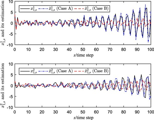
Figure 2. The curves of $x_{2,s}$ and ${\hat{x}}_{2,s}$.

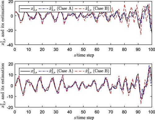
Figure 3. The curves of $x_{3,s}$ and ${\hat{x}}_{3,s}$.

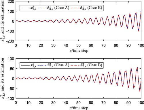
Figure 4. log(MSE) and upper bounds.

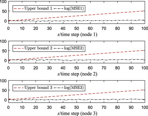
Figure 5. log(MSE) with/without compensation (500 iterations).

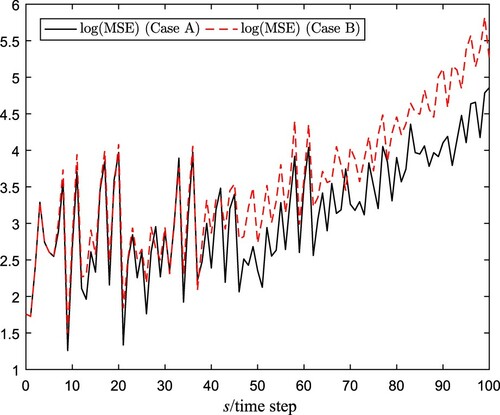
From the simulation results, we can see that the curves of recursive state estimation with predictive-based-compensation method come closer to the real nodes state than the estimation without predictive compensation. Then, one can conclude that the estimation performance of NPBSE algorithm is better than that of Case B without delay prediction-based method, which further demonstrates the advantages of the prediction idea and the NPBSE method. Moreover, as the iterations increase to 500, the MSE with the prediction updating rules (5(5) $\begin{array}{rl}{\hat{x}}_{j,s-d_{ij}+1|s-d_{ij}}& =A_{j,s-d_{ij}}{\hat{x}}_{j,s-d_{ij}},\\ {\hat{x}}_{j,s-d_{ij}+2|s-d_{ij}}& =A_{j,s-d_{ij}+1}{\hat{x}}_{j,s-d_{ij}+1|s-d_{ij}},\\ & ⋮\\ {\hat{x}}_{j,s-1|s-d_{ij}}& =A_{j,s-2}{\hat{x}}_{j,s-2|s-d_{ij}},\\ {\hat{x}}_{j,s|s-d_{ij}}& =A_{j,s-1}{\hat{x}}_{j,s-1|s-d_{ij}}.\end{array}$(5) ) should be smaller than another case clearly, which is consistent with the simulations provided in Figure 5. According to the above discussions, the negative effects caused by network-induced communication transmission delays and stochastic coupling are attenuated by the proposed new NPBSE algorithm.

In order to further reveal and check the algorithm performance, we conduct more experiments regarding the relationship of $\log (\mathrm{tr}\{{\mathcal{Z}}_{i,s+1}\})$ by considering different ${\beta }_{ij}$. For the comparison purpose, additional three cases are considered, i.e. Case I: ${\beta }_{ij}=0.68$, Case II: ${\beta }_{ij}=0.88$, Case III: ${\beta }_{ij}=0.98$. The related experiment results can be obtained and listed in Tables 1–3, where the result mentioned in Theorem 4.1 is clearly shown and illustrated. That is, the estimation accuracy becomes better when the phenomenon of stochastic coupling is not severe.

Table 1. log($\mathrm{tr}\{{\mathcal{Z}}_{1,s+1}\})$ and ${\beta }_{ij}$ (Node 1).

time(s)	···	65	66	67	68	69	···
Case I	···	30.389	30.82	31.195	31.842	32.363	···
Case II	···	32.587	33.047	33.457	34.133	34.68	···
Case III	···	33.666	34.138	34.565	35.255	35.815	···

Table 2. log($\mathrm{tr}\{{\mathcal{Z}}_{2,s+1}\})$ and ${\beta }_{ij}$ (Node 2).

time(s)	···	65	66	67	68	69	···
Case I	···	31.378	31.747	32.188	32.883	33.262	···
Case II	···	33.54	33.94	34.412	35.136	35.549	···
Case III	···	34.601	35.017	35.504	36.243	36.672	···

Table 3. log($\mathrm{tr}\{{\mathcal{Z}}_{3,s+1}\})$ and ${\beta }_{ij}$ (Node 3).

time(s)	···	65	66	67	68	69	···
Case I	···	31.487	32.135	32.481	32.987	33.585	···
Case II	···	33.528	34.262	34.55	35.101	35.803	···
Case III	···	34.54	35.314	35.576	36.149	36.9	···

6. Conclusions and future works

In this paper, the optimal estimation prediction-based issue has been handled for time-varying uncertain dynamical networks with communication transmission delays and stochastic coupling. The effect of communication transmission delays has been considered in the estimation between adjacent nodes in the network. Moreover, the Bernoulli distributed random variables have been utilized to model the stochastic coupling phenomenon and inaccuracy occurrence probabilities have been taken into account. A new time-varying state estimator has been constructed based on the prediction strategy. The presented main results have the following characteristics: 1) a hybrid predictive compensation method has been given, in which the stochastic coupling as well as communication transmission delays have been considered and well reflected in the state estimator; 2) the local optimized upper bound of the state estimation error covariance matrix has been established and the gain matrix of estimator has been designed; and 3) the monotonicity discussion has been analysed and the related mathematical proof has been given. Finally, the effectiveness of the state estimator has been discussed by providing some simulation comparisons. Accompanying with the rapid developments of the networked control technology, the analysis and optimization of complex dynamical networks become important. In particular, when the issue of the communication resources become a concern, the future research directions include the extension of the proposed active delay-prediction estimation method to deal with the state estimation problem of more general complex dynamical networks subject to different communication protocols as in Hu et al. (2017) and Zou, Wang et al. (2019).

Disclosure statement

No potential conflict of interest was reported by the authors.

Additional information

Funding

This work was supported in part by the National Natural Science Foundation of China [grant number 61673141], the European Regional Development Fund and Sr Cymru Fellowship [grant number 80761-USW-059], the Outstanding Youth Science Foundation of Heilongjiang Province of China [grant number JC2018001], the Fundamental Research Foundation for Universities of Heilongjiang Province of China [grant number 2019-KYYWF-0215] and the Alexander von Humboldt Foundation of Germany.

References

- An, B.-R., Liu, G.-P., & Tan, C. (2018). Group consensus control for networked multi-agent systems with communication delays. ISA Transactions, 76, 78–87. https://doi.org/https://doi.org/10.1016/j.isatra.2018.03.008
- Baran, L., & Rzysko, W. (2020). Application of a coarse-grained model for the design of complex supramolecular networks. Molecular Systems Design
Engineering, 5(2), 484–492. https://doi.org/https://doi.org/10.1039/C9ME00122K
- Bonello, J., Demarco, A., Farhat, I., Farrugia, L., & Sammut, C. V. (2020). Application of artificial neural networks for accurate determination of the complex permittivity of biological tissue. Sensors, 20(16), 1–18. https://doi.org/https://doi.org/10.3390/s20164640
- Bougofa, M., Bouafia, A., & Bellaouar, A. (2020). Availability assessment of complex systems under parameter uncertainty using dynamic evidential networks. International Journal of Performability Engineering, 16(4), 510–519. https://doi.org/https://doi.org/10.23940/ijpe.20.04.p2.510519
- Chen, D., Chen, W., Hu, J., & Liu, H. (2019). Variance-constrained filtering for discrete-time genetic regulatory networks with state delay and random measurement delay. International Journal of Systems Science, 50(2), 231–243. https://doi.org/https://doi.org/10.1080/00207721.2018.1542045
- Chen, W., Hu, J., Wu, Z., Yu, X., & Chen, D. (2020). Finite-time memory fault detection filter design for nonlinear discrete systems with deception attacks. International Journal of Systems Science, 51(8), 1464–1481. https://doi.org/https://doi.org/10.1080/00207721.2020.1765219
- Ding, R., Ujang, N., Bin Hamid, H., Abd Manan, M. S., Li, R., Albadareen, S. S. M., Nochian, A., & Wu, J. (2019). Application of complex networks theory in urban traffic network researches. Networks
- Hernandez-torres, J. E., Hernandez-gonzalez, S., Jimenez-garcia, J. A., & Figureoa-fernandez, V. (2020). Application of complex networks theory for transportation infrastructure analysis: celaya's city avenue network. Revista Eia, 17(33), 43–45. https://doi.org/https://doi.org/10.24050/reia.v17i33.1305
- Hu, J., Cui, Y., Lv, C., Chen, D., & Zhang, H. (2020). Robust adaptive sliding mode control for discrete singular systems with randomly occurring mixed time-delays under uncertain occurrence probabilities. International Journal of Systems Science, 51(6), 987–1006. https://doi.org/https://doi.org/10.1080/00207721.2020.1746439
- Hu, J., Liu, G.-P., Zhang, H., & Liu, H. (2020). On state estimation for nonlinear dynamical networks with random sensor delays and coupling strength under event-based communication mechanism. Information Sciences, 511, 265–283. https://doi.org/https://doi.org/10.1016/j.ins.2019.09.050
- Hu, J., Wang, Z., Alsaadi, F. E., & Hayat, T. (2017). Event-based filtering for time-varying nonlinear systems subject to multiple missing measurements with uncertain missing probabilities. Information Fusion, 38, 74–83. https://doi.org/https://doi.org/10.1016/j.inffus.2017.03.003
- Hu, J., Wang, Z., Chen, D., & Alsaadi, F. E. (2016). Estimation, filtering and fusion for networked systems with network-induced phenomena: new progress and prospects. Information Fusion, 31, 65–75. https://doi.org/https://doi.org/10.1016/j.inffus.2016.01.001
- Hu, J., Wang, Z., Liu, G.-P., Jia, C., & Williams, J. (2020). Event-triggered recursive state estimation for dynamical networks under randomly switching topologies and multiple missing measurements. Automatica, 115. Article No: 108908. doi:https://doi.org/10.1016/j.automatica.2020.108908
- Hu, J., Wang, Z., Liu, G.-P., & Zhang, H. (2020). Variance-constrained recursive state estimation for time-varying complex networks with quantized measurements and uncertain inner coupling. IEEE Transactions on Neural Networks and Learning Systems, 31(6), 1955–1967. https://doi.org/https://doi.org/10.1109/TNNLS.5962385
- Hu, J., Zhang, P., Kao, Y., Liu, H., & Chen, D. (2019). Sliding mode control for Markovian jump repeated scalar nonlinear systems with packet dropouts: The uncertain occurrence probabilities case. Applied Mathematics and Computation, 362. Article number: 124574. https://doi.org/https://doi.org/10.1016/j.amc.2019.124574
- Hu, J., Zhang, H., Yu, X., Liu, H., & Chen, D. (2019). Design of sliding-mode-based control for nonlinear systems with mixed-delays and packet losses under uncertain missing probability. IEEE Transactions on Systems, Man, and Cybernetics: Systems. doi:https://doi.org/10.1109/TSMC.2019.2919513
- Li, W., & J. Du, Y. J (2017). Recursive state estimation for complex networks with random coupling strength. Neurocomputing, 219, 1–8. https://doi.org/https://doi.org/10.1016/j.neucom.2016.08.095
- Li, W., Jia, Y., Du, J., & Fu, X. (2018). State estimation for nonlinearly coupled complex networks with application to multi-target tracking. Neurocomputing, 275, 1884–1892. https://doi.org/https://doi.org/10.1016/j.neucom.2017.10.012
- Liu, Y., Li, W., & Feng, J. (2018). Graph-theoretical method to the existence of stationary distribution of stochastic coupled systems. Journal of Dynamics and Differential Equations, 30(2), 667–685. https://doi.org/https://doi.org/10.1007/s10884-016-9566-y
- Locke, R., Kupis, S., Gehb, C. M., Platz, R., & Atamturktur, S. (2020). Applying uncertainty quantification to structural systems: parameter reduction for evaluating model complexity. Conference Proceedings of the Society for Experimental Mechanics Series, 3, 241–256. https://doi.org/https://doi.org/10.1007/978-3-030-12075-7
- Luo, Y., Deng, F., Ling, Z., & Cheng, Z. (2019). Local H∞ synchronization of uncertain complex networks via non-fragile state feedback control. Mathematics and Computers in Simulation, 155, 335–346. https://doi.org/https://doi.org/10.1016/j.matcom.2018.07.009
- Ma, L., Wang, Z., Han, Q.-L., & Liu, Y. (2018). Dissipative control for nonlinear Markovian jump systems with actuator failures and mixed time-delays. Automatica, 98, 358–362. https://doi.org/https://doi.org/10.1016/j.automatica.2018.09.028
- Ma, L., Wang, Z., Liu, Y., & Alsaadi, F. E. (2019). Distributed filtering for nonlinear time-delay systems over sensor networks subject to multiplicative link noises and switching topology. International Journal of Robust and Nonlinear Control, 29(10), 2941–2959. https://doi.org/https://doi.org/10.1002/rnc.v29.10
- Malinin, A., & Gales, M. (2018). Predictive uncertainty estimation via prior networks. Proceedings of the 32nd International Conference on Neural Information Processing Systems, December 2018, New York, United States, Pages 7047–7058.
- Mao, J., Sun, Y., Yi, X., Liu, H., & Ding, D. (2021). Recursive filtering of networked nonlinear systems: A survey. International Journal of Systems Science. doi:https://doi.org/10.1080/00207721.2020.1868615.
- Wang, L., An, M., Jia, L., & Qin, Y. (2019). Application of complex network principles to key station identification in railway network efficiency analysis. Journal of Advanced Transportation, 2019, 1–13. Article ID 1574136. https://doi.org/https://doi.org/10.1155/2019/1574136
- Wu, Y., & He, X. (2017). Secure consensus control for multi-agent systems with attacks and communication delays. IEEE/CAA Journal of Automatica Sinica, 4(1), 136–142. https://doi.org/https://doi.org/10.1109/JAS.2016.7510010
- Wu, Z.-G., Xu, Z., Shi, P., Chen, M. Z. Q., & Su, H. (2018). Nonfragile state estimation of quantized complex networks with switching topologies. IEEE Transactions on Neural Networks and Learning Systems, 29(10), 5111–5121. https://doi.org/https://doi.org/10.1109/TNNLS.2018.2790982
- Xia, J., Gao, S., Zhong, Y., Zhang, J., Gu, C., & Liu, Y. (2020). A novel fitting H∞ Kalman filter for nonlinear uncertain discrete-time systems based on fitting transformation. IEEE Access, 8, 10554–10568. https://doi.org/https://doi.org/10.1109/Access.6287639
- Xiong, Q., Lin, P., Ren, W., Yang, C., & Gui, W. (2018). Containment control for discrete-time multiagent systems with communication delays and switching topologies. IEEE Transactions on Cybernetics, 49(10), 3827–3830. https://doi.org/https://doi.org/10.1109/TCYB.6221036
- Xue, B., Wang, R., & Fei, S. (2020). Time-varying H∞ filtering for discrete-time switched systems with admissible edge-dependent average dwell time. Transactions of the Institute of Measurement and Control, 42(14), 2719–2732. https://doi.org/https://doi.org/10.1177/0142331220928889
- Zhao, J. (2018). Dynamic state estimation with model uncertainties using H∞ extended Kalman filter. IEEE Transactions on Power Systems, 33(1), 1099–1100. https://doi.org/https://doi.org/10.1109/TPWRS.2017.2688131
- Zhao, J., & Mili, L. (2019). A theoretical framework of robust H∞ unscented Kalman filter and its application to power system dynamic state estimation. IEEE Transactions on Signal Processing, 67(10), 2734–2746. https://doi.org/https://doi.org/10.1109/TSP.78
- Zou, L., Wang, Z., Dong, H., & Han, Q.-L. (2020). Moving horizon estimation with multi-rate measurements and correlated noises. International Journal of Robust and Nonlinear Control, 30(17), 7429–7445. https://doi.org/https://doi.org/10.1002/rnc.v30.17
- Zou, L., Wang, Z., Han, Q.-L., & Zhou, D. (2019). Moving horizon estimation of networked nonlinear systems with random access protocol. IEEE Transactions on Systems, Man, and Cybernetics-Systems. in press. doi:https://doi.org/10.1109/TSMC.2019.2918002
- Zou, L., Wang, Z., Hu, J., & Zhou, D.-H. (2020). Moving horizon estimation with unknown inputs under dynamic quantization effects. IEEE Transactions on Automatic Control, 65(12), 5368–5375. https://doi.org/https://doi.org/10.1109/TAC.9
- Zou, L., Wen, T., Wang, Z., Chen, L., & Roberts, C. (2019). State estimation for communication-based train control systems with CSMA protocol. IEEE Transactions on Intelligent Transportation Systems, 20(3), 843–854. https://doi.org/https://doi.org/10.1109/TITS.2018.2835655