H_∞ performance for load frequency control systems with random delays

Abstract

This paper investigates the problem of $H_{\mathrm{\infty }}$ performance analysis for PI-type load frequency control (LFC) of power systems with random delays. By taking the probability distribution characteristic of communication delays into account in the LFC design, the power systems with a PI controller are modelled as stochastic time-delay systems. Furthermore, a delay-product-type augmented Lyapunov-Krasovskii functional (LKF) is constructed, and a new extended reciprocally convex matrix inequality combining Wirtinger-based integral inequality with convex combination approach is utilized to reduce the conservatism of main results. As a result, less conservative $H_{\mathrm{\infty }}$ performance criteria are derived, which guarantee the asymptotically stable in the mean-square of the considered systems. Numerical examples are also provided to illustrate the superiority of our proposed methods.

Keywords:

• Random delays
• $H_{\mathrm{\infty }}$ performance
• load frequency control (LFC) systems
• Lyapunov-Krasovskii functional (LKF)
• extended reciprocally convex matrix inequality

1. Introduction

Load frequency control (LFC) has been widely utilized in large interconnected power systems with multiple control areas, which is one of the major measures to maintain the balance between the load and generation in a specified control area (Sharma et al., 2019; Wen et al., 2016; Yan & Xu, 2019). It should be noted that, dedicated communication channels have been made use of to transmit control signals between remote terminal units (RTUs) and a control centre in traditional centralized LFC schemes, the problems due to communication delays have been ignored by most previous research work (Fu et al., 2020; Jiang et al., 2012; Xiong et al., 2018; C. K. Zhang et al., 2013). However, with the emergence of numerous private networks and the employment of open communication networks, some challenging problems have appeared on account of limited network bandwidth, such as communication delays and data losses, which exerts potential threats on the stable operation of power systems (Peng et al., 2018; Sargolzaei et al., 2016; Singh et al., 2016). As a matter of fact, for a given communication channel based on transmission control protocol/internet protocol, communication delay is often random, and varies in an interval (Peng & Zhang, 2016). Generally speaking, random delays are characterized by means of Bernoulli-distributed stochastic variable, and this type of random interval delays could occur with a high probability in one subinterval and the opposite probability of occurring in another subinterval (Jia et al., 2019). Consequently, the delay intervals and corresponding occurrence probability should be fully considered, which is significant to obtain less conservative results. However, the probability distribution characteristic of communication delays was rarely considered in most existing studies. Therefore, it is of great significance to study the influence of random delays on LFC systems.

To LFC systems with random delays and load disturbance, the $H_{\mathrm{\infty }}$ performance level and the upper bounds of time delay are two major factors to judge the conservatism of the derived criteria. In order to further reduce the conservatism, sustained efforts have been made mainly on two aspects, one is to construct an appropriate LKF, the other is to estimate the derivatives of the LKF more accurately, such as delay-partitioning approach (Ko et al., 2018), augmented LKF (W. I. Lee et al., 2018; Zeng et al., 2019), LKF with triple-integral and quadruple-integral terms (Qian, Li, Chen, et al., 2020), LKF with delay-product terms (Li et al., 2019; Qian, Xing, et al., 2020; C. F. Shen et al., 2020; C. K. Zhang, He, Jiang, Wang, et al., 2017), Jensen's inequality (Qian, Li, Zhao, et al., 2020), Wirtinger-based integral inequality (Qian et al., 2019), free-matrix-based integral inequality (Zeng et al., 2015), auxiliary-function-based inequality (P. G. Park et al., 2015), Bessel-Legendre inequality (W. I. Lee et al., 2018; Seuret & Gouaisbaut, 2018) and reciprocally convex combination techniques in different forms (P. G. Park et al., 2011; C. K. Zhang, He, Jiang, Wang, et al., 2017; C. K. Zhang, He, Jiang, Wu, et al., 2017; R. M. Zhang et al., 2019). Furthermore, various $H_{\mathrm{\infty }}$ performance criteria for LFC systems have been put forward and researches on this problem are still going on. For instance, in Wen et al. (2016), by integrating the communication delays and event triggered control in the formulated model, and utilizing free-weighting matrix approach, the $H_{\mathrm{\infty }}$ performance criteria of LFC systems were derived. In Peng et al. (2018), an adaptive time-delay LFC model was developed, and reciprocally convex combination technique was applied in the derivation of main results, which can obtain improved $H_{\mathrm{\infty }}$ performance criteria and reduce the number of decision variables. By introducing the single and double integral items in LKF construction, and employing Jensen's inequality along with reciprocally convex combination approach, the delay-distribution-dependent $H_{\mathrm{\infty }}$ performance and stability criteria were presented in Peng and Zhang (2016). In Cheng et al. (2020), by considering transmission delays and denial-of-service attacks in the LFC design, and employing piecewise LKFs together with novel analysis methods, sufficient conditions were developed with $H_{\mathrm{\infty }}$ performance. In H. Zhang et al. (2020), a new model based on the area control error and time-varying delays was established, then an suitable LKF and extended Wirtinger's inequality was used, which had better $H_{\mathrm{\infty }}$ performance by the number of packets sent and average sampling period. By building an accurate model with a degree of packet losses and introducing an appropriate LKF, then exploiting Wirtinger-based inequality to estimate the integral terms, the desired $H_{\mathrm{\infty }}$ performance index of multi-area LFC systems was attained in Peng et al. (2017). It should be noted that, there is still plenty of room in how to coordinate LKF construction with estimating techniques efficiently, which helps to get $H_{\mathrm{\infty }}$ performance criteria with less conservative.

Inspired by above discussion, we further explore the $H_{\mathrm{\infty }}$ performance for PI-type LFC of power systems with random delays in this paper. The aim is to apply novel LKFs and explore new optimal analysis methods, by which the less conservative delay-dependent conditions and the desired $H_{\mathrm{\infty }}$ performance level can be obtained. The main advantages of this paper can be listed as follows:

• Delay-product-type functional approach is utilized in LKF construction, which make full use of the information about time-varying delay and its derivatives. By introducing state nonintegral terms with time-varying delay- dependent matrices and multiple integral terms, a novel augmented LKF is constructed. Meanwhile, the constraint that every Lyapunov matrix should be positive is relaxed, all of which contribute to reduce the conservatism of the main results.

• In order to estimate the infinitesimal operators of constructed LKF more accurately, the integral terms in single and double forms are separated precisely by using delay-partitioning method. Then the single integral terms are estimated by an extended reciprocally convex matrix inequality together with Wirtinger-based integral inequality, and the double integral items are estimated by Jensen's inequality, by which the constructed LKF and the estimating methods fit together effectively to reduce the conservatism of the main results.

Notation

Throughout this paper, ${\mathbb{R}}^n$ and ${\mathbb{R}}^{n\times m}$ denote the n-dimensional Euclidean space and the set of all $n\times m$ real matrices, respectively. $P>0\left(<0\right)$ means that P is a positive (negative) definite matrix. $\mathbb{E}\{\bullet \}$ is the mathematical expectation of •. $A^T$ and $A^{-1}$ represent the transpose and the inverse of A. $I_{n\times n}$ and $0_{n\times n}$ stand for $n\times n$ identity matrix and $n\times n$ zero matrix, respectively. $\ast$ in the matrix denotes the symmetric term. $diag\left\{\cdot \cdot \cdot \right\}$ denotes a block diagonal matrix, $col\left\{x_1,x_2,\dots ,x_n\right\}=[x_1^T{x}_2^T\cdots x_n^T{]}^T$ and $Sym\left\{X\right\}=X+X^T$.

2. Problem formulation and preliminaries

The schematic diagram of one-area delayed LFC systems with proportional-integral (PI) controller is presented in Figure 1,and its state-space equation is indicated as: (1) $\{\begin{array}{l}\dot{\tilde{x}}\left(t\right)=\tilde{A}\tilde{x}\left(t\right)+\tilde{B}u\left(t\right)+{\tilde{B}}_{\omega }\omega \left(t\right)\\ \tilde{y}\left(t\right)=\tilde{C}\tilde{x}\left(t\right)\end{array}$(1) where $\begin{array}{rl}& \tilde{x}\left(t\right)={\left[\mathrm{\Delta }f\mathrm{\Delta }{P}_m\mathrm{\Delta }{P}_v\right]}^T,\omega \left(t\right)=\mathrm{\Delta }{P}_d,\\ & \tilde{A}=\left[\begin{array}{ccc}-{\displaystyle \frac{D}{M}}& {\displaystyle \frac{1}{M}}& 0\\ 0& -{\displaystyle \frac{1}{T_{ch}}}& {\displaystyle \frac{1}{T_{ch}}}\\ -{\displaystyle \frac{1}{\hat{R}{T}_g}}& 0& -{\displaystyle \frac{1}{T_g}}\end{array}\right],\tilde{B}=\left[\begin{array}{c}0\\ 0\\ {\displaystyle \frac{1}{T_g}}\end{array}\right],\\ & {\tilde{B}}_{\omega }=\left[\begin{array}{c}-{\displaystyle \frac{1}{M}}\\ 0\\ 0\end{array}\right],\tilde{C}={\left[\begin{array}{c}\text{β}\\ 0\\ 0\end{array}\right]}^T\end{array}$and $\mathrm{\Delta }f$, $\mathrm{\Delta }{P}_m$, $\mathrm{\Delta }{P}_v$, $\mathrm{\Delta }{P}_d$ are the deviations of frequency, the turbine/generator mechanical output, generator valve position and the disturbance of load, respectively. M, D, $\hat{R}$, $T_{ch}$, $T_g$ denote the moment of inertia of the generator, the generator damping constant, speed droop, time constant of the turbine and time constant of the governor, respectively.

Figure 1. Schematic diagram of one-area LFC scheme.

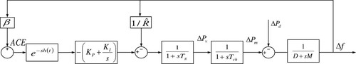
As we all know, there is no net tie-line power exchange in single-area power systems. It can be seen from Figure 1 that, as the output of the system (1(1) $\{\begin{array}{l}\dot{\tilde{x}}\left(t\right)=\tilde{A}\tilde{x}\left(t\right)+\tilde{B}u\left(t\right)+{\tilde{B}}_{\omega }\omega \left(t\right)\\ \tilde{y}\left(t\right)=\tilde{C}\tilde{x}\left(t\right)\end{array}$(1) ), the area control error (ACE) is denoted as: (2) $\tilde{y}\left(t\right)=ACE=\text{β}\mathrm{\Delta }f$(2) where $\text{β}>0$ is frequency bias factor. Moreover, ACE is also acted as the input of the designed controller, so the following PI-based controller can be designed: (3) $u\left(t\right)=-K_{P}ACE-K_I\int ACE$(3) where $K_P$ and $K_I$ are proportional and integral gains, and $\int ACE$ is the integration of ACE.

As depicted in Figure 1, the communication delay from ACE to the PI-based controller (3(3) $u\left(t\right)=-K_{P}ACE-K_I\int ACE$(3) ) is defined by an exponential block $e^{-sh\left(t\right)}$. Denote (4) $y\left(t\right)\stackrel{\mathrm{\Delta }}{=}{\left[\tilde{y}\left(t\right)\int \tilde{y}\left(t\right)\right]}^T,K\stackrel{\mathrm{\Delta }}{=}\left[K_P{K}_I\right]$(4) the PI-based controller (3(3) $u\left(t\right)=-K_{P}ACE-K_I\int ACE$(3) ) can be further written as: (5) $u\left(t\right)=-Ky\left(t-h\left(t\right)\right)$(5) where $h\left(t\right)$ is a time-varying delay satisfying: $0\le h\left(t\right)\le h,\dot{\phantom{a}}h\left(t\right)\le \mu$where h and $\mu <1$ are constants.

In this paper, the information about the probability distribution of time-varying delay $h\left(t\right)$ is employed.

Assumption 2.1

To describe the probability distribution of the time-varying delay $h\left(t\right)$, define two sets and functions by $\begin{array}{rl}& {\mathrm{\Omega }}_1=\left\{t:h\left(t\right)\in \left[0,h_0\right)\right\}\mathrm{a}\mathrm{n}\mathrm{d}\\ & {\mathrm{\Omega }}_2=\left\{t:h\left(t\right)\in \left[h_0,h\right]\right\}\\ & h_1\left(t\right)=\{\begin{array}{ll}h\left(t\right)& \mathrm{f}\mathrm{o}\mathrm{r}t\in {\mathrm{\Omega }}_1\\ {\overline{h}}_1& \mathrm{f}\mathrm{o}\mathrm{r}t\in {\mathrm{\Omega }}_2\end{array},\\ & h_2\left(t\right)=\{\begin{array}{ll}{\overline{h}}_2& \mathrm{f}\mathrm{o}\mathrm{r}t\in {\mathrm{\Omega }}_1\\ h\left(t\right)& \mathrm{f}\mathrm{o}\mathrm{r}t\in {\mathrm{\Omega }}_2\end{array}\\ & {\dot{h}}_1\left(t\right)\le {\mu }_1<1\mathrm{a}\mathrm{n}\mathrm{d}{\dot{h}}_2\left(t\right)\le {\mu }_2<1\end{array}$where $h_0\in \left[0,h\right]$, ${\overline{h}}_1\in \left[0,h_0\right)$, ${\overline{h}}_2\in \left[h_0,h\right]$. Obviously, ${\mathrm{\Omega }}_1\cup {\mathrm{\Omega }}_2={\mathbb{R}}^{+}$ and ${\mathrm{\Omega }}_1\cap {\mathrm{\Omega }}_2=set$. It is easy to know that $t\in {\mathrm{\Omega }}_1$ means the event $h\left(t\right)\in \left[0,h_0\right)$ occurs and $t\in {\mathrm{\Omega }}_2$ means the event $h\left(t\right)\in \left[h_0,h\right]$ occurs. Therefore, a stochastic variable $\alpha \left(t\right)$ can be defined as $\alpha \left(t\right)=\{\begin{array}{ll}1& \mathrm{f}\mathrm{o}\mathrm{r}t\in {\mathrm{\Omega }}_1,\\ 0& \mathrm{f}\mathrm{o}\mathrm{r}t\in {\mathrm{\Omega }}_2.\end{array}$

Assumption 2.2

The stochastic variable $\alpha \left(t\right)$ is a Bernoulli distributed sequence with $\{\begin{array}{ll}\mathrm{P}\mathrm{r}\mathrm{o}\mathrm{b}\left\{\alpha \left(t\right)=1\right\}& =\mathbb{E}\left\{\alpha \left(t\right)\right\}={\alpha }_0\\ \mathrm{P}\mathrm{r}\mathrm{o}\mathrm{b}\left\{\alpha \left(t\right)=0\right\}& =1-\mathbb{E}\left\{\alpha \left(t\right)\right\}=1-{\alpha }_0\end{array}$where $0⩽{\alpha }_0⩽1$ is a constant.

Remark 2.1

As is well known, the real power system is a system with high nonlinearity and time-varying characteristics. In practice, modern power systems usually require a wide area open communication network to transmit information concerned. The usage of these networks causes inevitable unreliable factors, such as time delays, packet losses, latent faults, and etc. Similarly, these nonlinear disturbances may occur randomly as a result of some environment reasons. Therefore, the stochastic variable $\alpha \left(t\right)$ is introduced in this paper to describe such randomly occurring phenomenon, which has universality and application prospect.

According to the above analysis, the following delay-distribution-dependent PI controller can be taken to replace the general form shown in (5(5) $u\left(t\right)=-Ky\left(t-h\left(t\right)\right)$(5) ): (6) $u\left(t\right)=-\alpha \left(t\right)Ky\left(t-h_1\left(t\right)\right)-\left(1-\alpha \left(t\right)\right)Ky\left(t-h_2\left(t\right)\right)$(6) Defining $x\left(t\right)=[\mathrm{\Delta }f\mathrm{\Delta }{P}_m\mathrm{\Delta }{P}_v\int ACE{]}^T$ and substituting (6(6) $u\left(t\right)=-\alpha \left(t\right)Ky\left(t-h_1\left(t\right)\right)-\left(1-\alpha \left(t\right)\right)Ky\left(t-h_2\left(t\right)\right)$(6) ) into (1(1) $\{\begin{array}{l}\dot{\tilde{x}}\left(t\right)=\tilde{A}\tilde{x}\left(t\right)+\tilde{B}u\left(t\right)+{\tilde{B}}_{\omega }\omega \left(t\right)\\ \tilde{y}\left(t\right)=\tilde{C}\tilde{x}\left(t\right)\end{array}$(1) ), it can be obtained: (7) $\{\begin{array}{rl}\dot{x}\left(t\right)& =Ax\left(t\right)-\alpha \left(t\right)BKCx\left(t-h_1\left(t\right)\right)-\left(1-\alpha \left(t\right)\right)\\ & BKCx\left(t-h_2\left(t\right)\right)+B_{\omega }\omega \left(t\right)\\ y\left(t\right)& =Cx\left(t\right)\\ x\left(t\right)& =\varphi \left(t\right),t\in \left[-h,0\right]\end{array}$(7) where $\begin{array}{rl}A& =\left[\begin{array}{cccc}{\displaystyle -\frac{D}{M}}& {\displaystyle \frac{1}{M}}& 0& 0\\ 0& -{\displaystyle \frac{1}{T_{ch}}}& {\displaystyle \frac{1}{T_{ch}}}& 0\\ {\displaystyle -\frac{1}{\hat{R}{T}_g}}& 0& -{\displaystyle \frac{1}{T_g}}& 0\\ \text{β}& 0& 0& 0\end{array}\right],B=\left[\begin{array}{c}0\\ 0\\ {\displaystyle -\frac{1}{T_g}}\\ 0\end{array}\right],\\ B_{\omega }& =\left[\begin{array}{c}-{\displaystyle \frac{1}{M}}\\ 0\\ 0\\ 0\end{array}\right],C={\left[\begin{array}{cc}\text{β}& 0\\ 0& 0\\ 0& 0\\ 0& 1\end{array}\right]}^T\end{array}$and $x\left(t\right)\in {\mathbb{R}}^n$ is the state vector. The initial condition $\varphi \left(t\right)$ denotes a vector-valued continuous function of $t\in \left[-h,0\right]$.

The main objective of this paper is to derive the less conservatism $H_{\mathrm{\infty }}$ performance criteria, and guarantee system (7(7) $\{\begin{array}{rl}\dot{x}\left(t\right)& =Ax\left(t\right)-\alpha \left(t\right)BKCx\left(t-h_1\left(t\right)\right)-\left(1-\alpha \left(t\right)\right)\\ & BKCx\left(t-h_2\left(t\right)\right)+B_{\omega }\omega \left(t\right)\\ y\left(t\right)& =Cx\left(t\right)\\ x\left(t\right)& =\varphi \left(t\right),t\in \left[-h,0\right]\end{array}$(7) ) is asymptotically mean-square stable. In order to obtain main results, the following definition and lemmas are required.

Definition 2.1

B. Shen et al., 2011

Given a scalar $\gamma >0$, under the zero initial condition, the system (7(7) $\{\begin{array}{rl}\dot{x}\left(t\right)& =Ax\left(t\right)-\alpha \left(t\right)BKCx\left(t-h_1\left(t\right)\right)-\left(1-\alpha \left(t\right)\right)\\ & BKCx\left(t-h_2\left(t\right)\right)+B_{\omega }\omega \left(t\right)\\ y\left(t\right)& =Cx\left(t\right)\\ x\left(t\right)& =\varphi \left(t\right),t\in \left[-h,0\right]\end{array}$(7) ) is said to be asymptotically mean-square stable with $H_{\mathrm{\infty }}$ performance level γ, if the following inequality holds $\mathbb{E}\left\{{\int }_0^{\mathrm{\infty }}{y}^T\left(t\right)y\left(t\right)\mathrm{d}t\right\}<{\gamma }^2{\int }_0^{\mathrm{\infty }}{\omega }^T\left(t\right)\omega \left(t\right)\mathrm{d}t.$

Lemma 2.1

Qian et al., 2019

For a positive definite matrix R>0, the following inequality holds for all continuously differential function $\omega \left(s\right)$ in $\left[\alpha ,\text{β}\right]\to {\mathbb{R}}^n$: $\begin{array}{rl}{\int }_{\alpha }^{\text{β}}{\omega }^T\left(s\right)R\omega \left(s\right)\mathrm{d}s& ⩾\frac{1}{\text{β}-\alpha }{\left({\int }_{\alpha }^{\text{β}}\omega \left(s\right)\mathrm{d}s\right)}^T\\ & \times R\left({\int }_{\alpha }^{\text{β}}\omega \left(s\right)\mathrm{d}s\right)+\frac{3}{\text{β}-\alpha }{\varpi }^{T}R\varpi \end{array}$where $\varpi ={\int }_{\alpha }^{\text{β}}\omega \left(s\right)\mathrm{d}s-\frac{2}{\text{β}-\alpha }{\int }_{\alpha }^{\text{β}}{\int }_{\theta }^{\text{β}}\omega \left(s\right)\mathrm{d}s\mathrm{d}\theta$.

Lemma 2.2

C. K. Zhang, He, Jiang, Wu, et al., 2017

For a real scalar $\alpha \in \left(0,1\right)$, symmetric matrices ${\chi }_1>0$, ${\chi }_2>0$, and any matrices $S_1$ and $S_2$, the following matrix inequality holds: $\begin{array}{rl}& \left[\begin{array}{cc}{\displaystyle \frac{1}{\alpha }{\chi }_1}& 0\\ 0& {\displaystyle \frac{1}{1-\alpha }{\chi }_2}\end{array}\right]\\ & ⩾\left[\begin{array}{cc}{\chi }_1+\left(1-\alpha \right){\mathrm{\Im }}_1& \left(1-\alpha \right)S_1+\alpha S_2\\ \ast & {\chi }_2+\alpha {\mathrm{\Im }}_2\end{array}\right]\end{array}$where ${\mathrm{\Im }}_1={\chi }_1-S_2{{\chi }_2}^{-1}{S_2}^T$, ${\mathrm{\Im }}_2={\chi }_2-{S_1}^T{{\chi }_1}^{-1}{S}_1$.

3. Main results

In this section, by constructing a novel delay-product augmented LKF and employing appropriate analytical methods, some improved $H_{\mathrm{\infty }}$ performance and stability criteria for the considered systems are given. Some notations are shown to simplify the representation of the following parts: $\begin{array}{rl}{\phi }_1\left(t\right)& ={\int }_{t-h_1\left(t\right)}^t\frac{x\left(s\right)}{h_1\left(t\right)}\mathrm{d}s,\\ {\phi }_2\left(t\right)& ={\int }_{t-h_0}^{t-h_1\left(t\right)}\frac{x\left(s\right)}{h_0-h_1\left(t\right)}\mathrm{d}s,\\ {\phi }_3\left(t\right)& ={\int }_{t-h_2\left(t\right)}^{t-h_0}\frac{x\left(s\right)}{h_2\left(t\right)-h_0}\mathrm{d}s,\\ {\phi }_4\left(t\right)& ={\int }_{t-h}^{t-h_2\left(t\right)}\frac{x\left(s\right)}{h-h_2\left(t\right)}\mathrm{d}s,\\ {\phi }_5\left(t\right)& ={\int }_{t-h_1\left(t\right)}^t{\int }_{\theta }^t\frac{x\left(s\right)}{h_1\left(t\right)}\mathrm{d}s\mathrm{d}\theta ,\\ {\phi }_6\left(t\right)& ={\int }_{t-h_0}^{t-h_1\left(t\right)}{\int }_{\theta }^{t-h_1\left(t\right)}\frac{x\left(s\right)}{h_0-h_1\left(t\right)}\mathrm{d}s\mathrm{d}\theta ,\\ {\phi }_7\left(t\right)& ={\int }_{t-h_2\left(t\right)}^{t-h_0}{\int }_{\theta }^{t-h_0}\frac{x\left(s\right)}{h_2\left(t\right)-h_0}\mathrm{d}s\mathrm{d}\theta ,\\ {\phi }_8\left(t\right)& ={\int }_{t-h}^{t-h_2\left(t\right)}{\int }_{\theta }^{t-h_2\left(t\right)}\frac{x\left(s\right)}{h-h_2\left(t\right)}\mathrm{d}s\mathrm{d}\theta ,\\ \xi \left(t\right)& =col\{x\left(t\right),x\left(t-h_1\left(t\right)\right),x\left(t-h_0\right),\\ & x\left(t-h_2\left(t\right)\right),x\left(t-h\right),\dot{x}\left(t\right),\dot{x}\left(t-h_1\left(t\right)\right),\\ & \dot{\phantom{a}}x\left(t-h_0\right),\dot{x}\left(t-h_2\left(t\right)\right),\dot{x}\left(t-h\right),\\ & {\phi }_1\left(t\right),{\phi }_2\left(t\right),{\phi }_3\left(t\right),{\phi }_4\left(t\right),{\phi }_5\left(t\right),\\ & {\phi }_6\left(t\right),{\phi }_7\left(t\right),{\phi }_8\left(t\right),\omega \left(t\right)\}.\end{array}$

Theorem 3.1

For some given positive scalars ${\alpha }_0$, $h_0$, h, ${\mu }_1$, ${\mu }_2$, γ and a matrix K, system (7(7) $\{\begin{array}{rl}\dot{x}\left(t\right)& =Ax\left(t\right)-\alpha \left(t\right)BKCx\left(t-h_1\left(t\right)\right)-\left(1-\alpha \left(t\right)\right)\\ & BKCx\left(t-h_2\left(t\right)\right)+B_{\omega }\omega \left(t\right)\\ y\left(t\right)& =Cx\left(t\right)\\ x\left(t\right)& =\varphi \left(t\right),t\in \left[-h,0\right]\end{array}$(7) ) is asymptotically mean-square stable with $H_{\mathrm{\infty }}$ performance γ, if there exist symmetric positive definite matrices $W_m,M_m\in {\mathbb{R}}^{2n\times 2n}$ $\left(m=1,2\right)$, symmetric matrices $P\in {\mathbb{R}}^{9n\times 9n}$, $L_i\in {\mathbb{R}}^{2n\times 2n}$ $\left(i=1,2,3,4\right)$ and $Q_j\in {\mathbb{R}}^{2n\times 2n}$ $\left(j=1,2,\dots ,8\right)$, and any matrices $T_k,S_k$ $\left(k=1,2,3,4\right)$, ${\mathcal{N}}_1$ and ${\mathcal{N}}_2$ with appropriate dimensions, such that the following LMIs hold: (8) $\begin{array}{rl}& \left[\begin{array}{ccc}{\displaystyle \sum _{i=1}^8{\mathrm{\Xi }}_{i\left[h_1\left(t\right)=0,h_2\left(t\right)=h_0\right]}+\psi +\mathrm{\aleph }}& {\mathcal{F}}_1^T{S}_2& {\mathcal{F}}_5^T{S}_4\\ \ast & -{\overline{\vartheta }}_2& 0\\ \ast & \ast & -{\overline{\vartheta }}_4\end{array}\right]<0\end{array}$(8) (9) $\begin{array}{rl}& \left[\begin{array}{ccc}{\displaystyle \sum _{i=1}^8{\mathrm{\Xi }}_{i\left[h_1\left(t\right)=0,h_2\left(t\right)=h\right]}+\psi +\mathrm{\aleph }}& {\mathcal{F}}_1^T{S}_2& {\mathcal{F}}_7^T{S}_3^T\\ \ast & -{\overline{\vartheta }}_2& 0\\ \ast & \ast & -{\overline{\vartheta }}_3\end{array}\right]<0\end{array}$(9) (10) $\begin{array}{rl}& \left[\begin{array}{ccc}{\displaystyle \sum _{i=1}^8{\mathrm{\Xi }}_{i\left[h_1\left(t\right)=h_0,h_2\left(t\right)=h_0\right]}+\psi +\mathrm{\aleph }}& {\mathcal{F}}_3^T{S}_1^T& {\mathcal{F}}_5^T{S}_4\\ \ast & -{\overline{\vartheta }}_1& 0\\ \ast & \ast & -{\overline{\vartheta }}_4\end{array}\right]<0\end{array}$(10) (11) $\begin{array}{rl}& \left[\begin{array}{ccc}{\displaystyle \sum _{i=1}^8{\mathrm{\Xi }}_{i\left[h_1\left(t\right)=h_0,h_2\left(t\right)=h\right]}+\psi +\mathrm{\aleph }}& {\mathcal{F}}_3^T{S}_1^T& {\mathcal{F}}_7^T{S}_3^T\\ \ast & -{\overline{\vartheta }}_1& 0\\ \ast & \ast & -{\overline{\vartheta }}_3\end{array}\right]<0\end{array}$(11) (12) $\begin{array}{rl}& {\mathrm{\Psi }}_{\left[h_1\left(t\right),h_2\left(t\right)\right]}>0,\mathrm{\forall }{h}_1\left(t\right)\in \left\{0,h_0\right\},h_2\left(t\right)\in \left\{h_0,h\right\}\end{array}$(12) (13) $\begin{array}{rl}& Q_1\left(t\right)>0,Q_3\left(t\right)>0,Q_5\left(t\right)>0,Q_7\left(t\right)>0\end{array}$(13) (14) $\begin{array}{rl}& {\overline{\vartheta }}_1>0,{\overline{\vartheta }}_2>0,{\overline{\vartheta }}_3>0,{\overline{\vartheta }}_4>0\end{array}$(14) where $\begin{array}{rl}{\mathrm{\Xi }}_{1\left[h_1\left(t\right),h_2\left(t\right)\right]}& =Sym\left\{{\mathrm{\Pi }}_1^{T}P{\mathrm{\Pi }}_2\right\}\\ {\mathrm{\Xi }}_{2\left[h_1\left(t\right),h_2\left(t\right)\right]}& =2{\mathrm{\Pi }}_3^T{L}_1{\mathrm{\Pi }}_4+2{\mathrm{\Pi }}_5^T{L}_2{\mathrm{\Pi }}_6+2{\mathrm{\Pi }}_7^T{L}_3{\mathrm{\Pi }}_8\\ & +2{\mathrm{\Pi }}_9^T{L}_4{\mathrm{\Pi }}_{10}+{\mu }_1{\mathrm{\Pi }}_3^T{L}_1{\mathrm{\Pi }}_3-{\mu }_1{\mathrm{\Pi }}_5^T{L}_2{\mathrm{\Pi }}_5\\ & +{\mu }_2{\mathrm{\Pi }}_7^T{L}_3{\mathrm{\Pi }}_7-{\mu }_2{\mathrm{\Pi }}_9^T{L}_4{\mathrm{\Pi }}_9\\ {\mathrm{\Xi }}_{3\left[h_1\left(t\right),h_2\left(t\right)\right]}& ={\mathrm{\Pi }}_{11}^T{Q}_1\left(t\right){\mathrm{\Pi }}_{11}-{\mathrm{\Pi }}_{12}^T{Q}_7\left(t\right){\mathrm{\Pi }}_{12}\\ & -{\mathrm{\Pi }}_{13}^T\left(Q_3\left(t\right)-Q_5\left(t\right)\right){\mathrm{\Pi }}_{13}\\ & -\left(1-{\mu }_1\right){\mathrm{\Pi }}_{14}^T\left(Q_1\left(t\right)-Q_3\left(t\right)\right){\mathrm{\Pi }}_{14}\\ & -\left(1-{\mu }_2\right){\mathrm{\Pi }}_{15}^T\left(Q_5\left(t\right)-Q_7\left(t\right)\right){\mathrm{\Pi }}_{15}\\ {\mathrm{\Xi }}_{4\left[h_1\left(t\right),h_2\left(t\right)\right]}& ={\mathrm{\Pi }}_{11}^T\{h_0^2{W}_1+{\left(h-h_0\right)}^2{W}_2+\frac{h_0^2}{2}{M}_1\\ & +\frac{{\left(h-h_0\right)}^2}{2}{M}_2\}{\mathrm{\Pi }}_{11}\\ {\mathrm{\Xi }}_{5\left[h_1\left(t\right),h_2\left(t\right)\right]}& =Sym\left\{h_0{\mathcal{F}}_1^T{\overline{\vartheta }}_1{\mathcal{F}}_2\right\}+h_0{h}_1\left(t\right){\mathcal{F}}_2^T{\overline{\vartheta }}_1{\mathcal{F}}_2\end{array}$ $\begin{array}{rl}& +Sym\left\{h_0{\mathcal{F}}_3^T{\overline{\vartheta }}_2{\mathcal{F}}_4\right\}\\ & +h_0\left(h_0-h_1\left(t\right)\right){\mathcal{F}}_4^T{\overline{\vartheta }}_2{\mathcal{F}}_4\\ & +Sym\left\{\left(h-h_0\right){\mathcal{F}}_5^T{\overline{\vartheta }}_3{\mathcal{F}}_6\right\}\\ & +\left(h-h_0\right)\left(h_2\left(t\right)-h_0\right){\mathcal{F}}_6^T{\overline{\vartheta }}_3{\mathcal{F}}_6\\ & +Sym\left\{\left(h-h_0\right){\mathcal{F}}_7^T{\overline{\vartheta }}_4{\mathcal{F}}_8\right\}\\ & +\left(h-h_0\right)\left(h-h_2\left(t\right)\right){\mathcal{F}}_8^T{\overline{\vartheta }}_4{\mathcal{F}}_8\\ {\mathrm{\Xi }}_{6\left[h_1\left(t\right),h_2\left(t\right)\right]}& =-\frac{2h_0-h_1\left(t\right)}{h_0}{\mathcal{F}}_1^T{\overline{\vartheta }}_1{\mathcal{F}}_1\\ & -\frac{h_0+h_1\left(t\right)}{h_0}{\mathcal{F}}_3^T{\overline{\vartheta }}_2{\mathcal{F}}_3\\ & -\frac{h_0-h_1\left(t\right)}{h_0}Sym\left\{{\mathcal{F}}_1^T{S}_1{\mathcal{F}}_3\right\}\\ & -\frac{h_1\left(t\right)}{h_0}Sym\left\{{\mathcal{F}}_1^T{S}_2{\mathcal{F}}_3\right\}\\ {\mathrm{\Xi }}_{7\left[h_1\left(t\right),h_2\left(t\right)\right]}& =-\frac{2h-h_0-h_2\left(t\right)}{h-h_0}{\mathcal{F}}_5^T{\overline{\vartheta }}_3{\mathcal{F}}_5\end{array}$ $\begin{array}{rl}& -\frac{h-2h_0+h_2\left(t\right)}{h-h_0}{\mathcal{F}}_7^T{\overline{\vartheta }}_4{\mathcal{F}}_7\\ & -\frac{h-h_2\left(t\right)}{h-h_0}Sym\left\{{\mathcal{F}}_5^T{S}_3{\mathcal{F}}_7\right\}\\ & -\frac{h_2\left(t\right)-h_0}{h-h_0}Sym\left\{{\mathcal{F}}_5^T{S}_4{\mathcal{F}}_7\right\}\\ {\mathrm{\Xi }}_{8\left[h_1\left(t\right),h_2\left(t\right)\right]}& =-2{\mathrm{\Pi }}_{16}^T{M}_1{\mathrm{\Pi }}_{16}-2{\mathrm{\Pi }}_{17}^T{M}_1{\mathrm{\Pi }}_{17}\\ & -2{\mathrm{\Pi }}_{18}^T{M}_2{\mathrm{\Pi }}_{18}-2{\mathrm{\Pi }}_{19}^T{M}_2{\mathrm{\Pi }}_{19}\\ \psi & =Sym\left\{\mathrm{{\rm Y}}\mathrm{\Theta }\right\},\\ \mathrm{{\rm Y}}& =e_1^T{\mathcal{N}}_1+e_6^T{\mathcal{N}}_2,\mathrm{\aleph }=e_1^T{C}^{T}C{e}_1-{\gamma }^2{e}_{19}^T{e}_{19}\\ \mathrm{\Theta }& =A{e}_1-{\alpha }_{0}BKC{e}_2-\left(1-{\alpha }_0\right)BKC{e}_4\\ & +B_{\omega }{e}_{19}-e_6\\ {\mathrm{\Pi }}_1& =[e_1^T{h}_1\left(t\right)e_{11}^T\left(h_0-h_1\left(t\right)\right)e_{12}^T\\ & \left(h_2\left(t\right)-h_0\right)e_{13}^T\left(h-h_2\left(t\right)\right)e_{14}^T{h}_1\left(t\right)e_{15}^T\end{array}$ $\begin{array}{rl}& \left(h_0-h_1\left(t\right)\right)e_{16}^T\left(h_2\left(t\right)-h_0\right)e_{17}^T\\ & \left(h-h_2\left(t\right)\right)e_{18}^T{]}^T\\ {\mathrm{\Pi }}_2& =[e_6^T{e}_1^T-\left(1-{\mu }_1\right)e_2^T\left(1-{\mu }_1\right)e_2^T-e_3^T\\ & e_3^T-\left(1-{\mu }_2\right)e_4^T\left(1-{\mu }_2\right)e_4^T-e_5^T\\ & h_1\left(t\right)e_1^T-\left(1-{\mu }_1\right)h_1\left(t\right)e_{11}^T\\ & \left(1-{\mu }_1\right)\left(h_0-h_1\left(t\right)\right)e_2^T-\left(h_0-h_1\left(t\right)\right)e_{12}^T\\ & \left(h_2\left(t\right)-h_0\right)e_3^T-\left(1-{\mu }_2\right)\left(h_2\left(t\right)-h_0\right)e_{13}^T\\ & \left(1-{\mu }_2\right)\left(h-h_2\left(t\right)\right)e_4^T-\left(h-h_2\left(t\right)\right)e_{14}^T{]}^T\\ {\mathrm{\Pi }}_3& =[e_1^T{e}_{11}^T{]}^T,{\mathrm{\Pi }}_5=[e_1^T{e}_{12}^T{]}^T,\\ {\mathrm{\Pi }}_7& =[e_1^T{e}_{13}^T{]}^T,{\mathrm{\Pi }}_9=[e_1^T{e}_{14}^T{]}^T\end{array}$ $\begin{array}{rl}{\mathrm{\Pi }}_4& =[h_1\left(t\right)e_6^T{e}_1^T-\left(1-{\mu }_1\right)e_2^T-{\mu }_1{e}_{11}^T{]}^T,\\ {\mathrm{\Pi }}_6& =[\left(h_0-h_1\left(t\right)\right)e_6^T\\ & \left(1-{\mu }_1\right)e_2^T-e_3^T+{\mu }_1{e}_{12}^T{]}^T\\ {\mathrm{\Pi }}_8& =\left[\right(h_2\left(t\right)-h_0)e_6^T\\ & e_3^T-\left(1-{\mu }_2\right)e_4^T-{\mu }_2{e}_{13}^T{]}^T\\ {\mathrm{\Pi }}_{10}& =\left[\right(h-h_2\left(t\right))e_6^T\\ & \left(1-{\mu }_2\right)e_4^T-e_5^T+{\mu }_2{e}_{14}^T{]}^T\\ {\mathrm{\Pi }}_{11}& =[e_1^T{e}_6^T{]}^T,{\mathrm{\Pi }}_{12}=[e_5^T{e}_{10}^T{]}^T,\\ {\mathrm{\Pi }}_{13}& =[e_3^T{e}_8^T{]}^T,{\mathrm{\Pi }}_{14}=[e_2^T{e}_7^T{]}^T\\ {\mathrm{\Pi }}_{15}& =[e_4^T{e}_9^T{]}^T,{\mathrm{\Pi }}_{16}=[e_{15}^T{e}_1^T-e_{11}^T{]}^T,\end{array}$ $\begin{array}{rl}{\mathrm{\Pi }}_{17}& =[e_{16}^T{e}_2^T-e_{12}^T{]}^T\\ {\mathrm{\Pi }}_{18}& =[e_{17}^T{e}_3^T-e_{13}^T{]}^T,\\ {\mathrm{\Pi }}_{19}& =[e_{18}^T{e}_4^T-e_{14}^T{]}^T\\ {\mathcal{F}}_1& =[0e_1^T-e_2^T-2e_{15}^T-e_1^T-e_2^T+2e_{11}^T{]}^T,\\ {\mathcal{F}}_3& =[0e_2^T-e_3^T-2e_{16}^T-e_2^T-e_3^T+2e_{12}^T{]}^T\\ {\mathcal{F}}_5& =[0e_3^T-e_4^T-2e_{17}^T-e_3^T-e_4^T+2e_{13}^T{]}^T,\\ {\mathcal{F}}_7& =[0e_4^T-e_5^T-2e_{18}^T-e_4^T-e_5^T+2e_{14}^T{]}^T\\ {\mathcal{F}}_2& =[e_{11}^{T}0e_{11}^{T}0{]}^T,\\ {\mathcal{F}}_4& =[e_{12}^{T}0e_{12}^{T}0{]}^T\\ {\mathcal{F}}_6& =[e_{13}^{T}0e_{13}^{T}0{]}^T,\\ & {\mathcal{F}}_8=[e_{14}^{T}0e_{14}^{T}0{]}^T\end{array}$ $\begin{array}{rl}{\overline{\vartheta }}_1& =\mathrm{d}\mathrm{i}\mathrm{a}\mathrm{g}\left\{{\vartheta }_1,3{\vartheta }_1\right\},{\overline{\vartheta }}_2=\mathrm{d}\mathrm{i}\mathrm{a}\mathrm{g}\left\{{\vartheta }_2,3{\vartheta }_2\right\},\\ {\overline{\vartheta }}_3& =\mathrm{d}\mathrm{i}\mathrm{a}\mathrm{g}\left\{{\vartheta }_3,3{\vartheta }_3\right\},{\overline{\vartheta }}_4=\mathrm{d}\mathrm{i}\mathrm{a}\mathrm{g}\left\{{\vartheta }_4,3{\vartheta }_4\right\}\\ {\vartheta }_1& =\frac{{\mu }_1}{h_0}{Q}_2+W_1+\frac{h_0-h_1\left(t\right)}{h_0}{M}_1,\\ {\vartheta }_2& =\frac{{\mu }_1}{h_0}{Q}_4+W_1,\\ {\vartheta }_3& =\frac{{\mu }_2}{h-h_0}{Q}_6+W_2+\frac{h-h_2\left(t\right)}{h-h_0}{M}_2,\\ {\vartheta }_4& =\frac{{\mu }_2}{h-h_0}{Q}_8+W_2\\ {\mathrm{\Psi }}_{\left[h_1\left(t\right),h_2\left(t\right)\right]}& =[\begin{array}{cc}P+L_A& {\displaystyle \frac{\sqrt{h_1\left(t\right)}}{h_0}{\mathcal{A}}_3^T{T}_1^T}\\ \ast & L_1\\ \ast & \ast \\ \ast & \ast \\ \ast & \ast \end{array}\end{array}$ $\begin{array}{rl}& \begin{array}{cc}{\displaystyle \frac{\sqrt{h_0-h_1\left(t\right)}}{h_0}{\mathcal{A}}_2^T{T}_2}& {\displaystyle \frac{\sqrt{h_2\left(t\right)-h_0}}{h-h_0}{\mathcal{A}}_5^T{T}_3^T}\\ 0& 0\\ L_2& 0\\ \ast & L_3\\ \ast & \ast \end{array}\\ & \begin{array}{c}{\displaystyle \frac{\sqrt{h-h_2\left(t\right)}}{h-h_0}{\mathcal{A}}_4^T{T}_4}\\ 0\\ 0\\ 0\\ L_4\end{array}]\\ L_A& ={\mathcal{A}}_1^T(h_1\left(t\right)L_1+\left(h_0-h_1\left(t\right)\right)L_2\end{array}$ $\begin{array}{rl}& +\left(h_2\left(t\right)-h_0\right)L_3+\left(h-h_2\left(t\right)\right)L_4){\mathcal{A}}_1\\ & +Sym\{{\mathcal{A}}_1^T{L}_1{\mathcal{A}}_2+{\mathcal{A}}_1^T{L}_2{\mathcal{A}}_3\\ & +{\mathcal{A}}_1^T{L}_3{\mathcal{A}}_4+{\mathcal{A}}_1^T{L}_4{\mathcal{A}}_5\}\\ & +\frac{2h_0-h_1\left(t\right)}{h_0^2}{\mathcal{A}}_2^T{L}_1{\mathcal{A}}_2\\ & +\frac{h_0+h_1\left(t\right)}{h_0^2}{\mathcal{A}}_3^T{L}_2{\mathcal{A}}_3\\ & +\frac{2h-h_0-h_2\left(t\right)}{{\left(h-h_0\right)}^2}{\mathcal{A}}_4^T{L}_3{\mathcal{A}}_4\\ & +\frac{h-2h_0+h_2\left(t\right)}{{\left(h-h_0\right)}^2}{\mathcal{A}}_5^T{L}_4{\mathcal{A}}_5\\ & +Sym\{\frac{h_0-h_1\left(t\right)}{h_0^2}{\mathcal{A}}_2^T{T}_1{\mathcal{A}}_3\\ & +\frac{h_1\left(t\right)}{h_0^2}{\mathcal{A}}_2^T{T}_2{\mathcal{A}}_3+\frac{h-h_2\left(t\right)}{{\left(h-h_0\right)}^2}{\mathcal{A}}_4^T{T}_3{\mathcal{A}}_5\\ & +\frac{h_2\left(t\right)-h_0}{{\left(h-h_0\right)}^2}{\mathcal{A}}_4^T{T}_4{\mathcal{A}}_5\}\\ {\mathcal{A}}_1& =col\left\{{\overline{e}}_1,0\right\},{\mathcal{A}}_2=col\left\{0,{\overline{e}}_2\right\},\end{array}$ $\begin{array}{rl}{\mathcal{A}}_3& =col\left\{0,{\overline{e}}_3\right\},{\mathcal{A}}_4=col\left\{0,{\overline{e}}_4\right\},\\ {\mathcal{A}}_5& =col\left\{0,{\overline{e}}_5\right\}\\ e_i& =[0_{n\times \left(i-1\right)n}{I}_{n\times n}{0}_{n\times \left(19-i\right)n}{]}^T,\\ i& =1,2,\dots ,19\\ {\overline{e}}_i& =[0_{n\times \left(i-1\right)n}{I}_{n\times n}{0}_{n\times \left(9-i\right)n}{]}^T,\\ i& =1,2,\dots ,9.\end{array}$

Proof.

Define the Lyapunov-Krasovskii functional candidate as follows: (15) $V\left(x_t\right)=\sum _{i=1}^5{V}_i\left(x_t\right)$(15) where (16) $\begin{array}{rl}{V}_1\left(x_t\right)& ={\eta }_1^T\left(t\right)P{\eta }_1\left(t\right)\end{array}$(16) (17) $\begin{array}{rl}{V}_2\left(x_t\right)& ={\eta }_2^T\left(t\right)L_1\left(t\right){\eta }_2\left(t\right)+{\eta }_3^T\left(t\right)L_2\left(t\right){\eta }_3\left(t\right)\\ & +{\eta }_4^T\left(t\right)L_3\left(t\right){\eta }_4\left(t\right)+{\eta }_5^T\left(t\right)L_4\left(t\right){\eta }_5\left(t\right)\end{array}$(17) (18) $\begin{array}{rl}{V}_3\left(x_t\right)& ={\int }_{t-h_1\left(t\right)}^t{\eta }_6^T\left(s\right)Q_1\left(t\right){\eta }_6\left(s\right)\mathrm{d}s\\ & +{\int }_{t-h_0}^{t-h_1\left(t\right)}{\eta }_6^T\left(s\right)Q_3\left(t\right){\eta }_6\left(s\right)\mathrm{d}s\\ & +{\int }_{t-h_2\left(t\right)}^{t-h_0}{\eta }_6^T\left(s\right)Q_5\left(t\right){\eta }_6\left(s\right)\mathrm{d}s\\ & +{\int }_{t-h}^{t-h_2\left(t\right)}{\eta }_6^T\left(s\right)Q_7\left(t\right){\eta }_6\left(s\right)\mathrm{d}s\end{array}$(18) (19) $\begin{array}{rl}{V}_4\left(x_t\right)& =h_0{\int }_{-h_0}^0{\int }_{t+\theta }^t{\eta }_6^T\left(s\right)W_1{\eta }_6\left(s\right)\mathrm{d}s\mathrm{d}\theta \\ & +\left(h-h_0\right){\int }_{-h}^{-h_0}{\int }_{t+\theta }^t{\eta }_6^T\left(s\right)W_2{\eta }_6\left(s\right)\mathrm{d}s\mathrm{d}\theta \end{array}$(19) (20) $\begin{array}{rl}{V}_5\left(x_t\right)& ={\int }_{t-h_0}^t{\int }_{\theta }^t{\int }_u^t{\eta }_6^T\left(s\right)M_1{\eta }_6\left(s\right)\mathrm{d}s\mathrm{d}u\mathrm{d}\theta \\ & +{\int }_{t-h}^{t-h_0}{\int }_{\theta }^{t-h_0}{\int }_u^t{\eta }_6^T\left(s\right)M_2{\eta }_6\left(s\right)\mathrm{d}s\mathrm{d}u\mathrm{d}\theta \end{array}$(20) with $\begin{array}{rl}{\eta }_1\left(t\right)& =col\{x\left(t\right),h_1\left(t\right){\phi }_1\left(t\right),\left(h_0-h_1\left(t\right)\right){\phi }_2\left(t\right),\\ & \left(h_2\left(t\right)-h_0\right){\phi }_3\left(t\right),\left(h-h_2\left(t\right)\right){\phi }_4\left(t\right),\\ & h_1\left(t\right){\phi }_5\left(t\right),\left(h_0-h_1\left(t\right)\right){\phi }_6\left(t\right),\left(h_2\left(t\right)-h_0\right){\phi }_7\left(t\right),\\ & \left(h-h_2\left(t\right)\right){\phi }_8\left(t\right)\}\\ {\eta }_2\left(t\right)& =col\left\{x\left(t\right),{\phi }_1\left(t\right)\right\},{\eta }_3\left(t\right)=col\left\{x\left(t\right),{\phi }_2\left(t\right)\right\},\\ {\eta }_4\left(t\right)& =col\left\{x\left(t\right),{\phi }_3\left(t\right)\right\}\\ {\eta }_5\left(t\right)& =col\left\{x\left(t\right),{\phi }_4\left(t\right)\right\},{\eta }_6\left(s\right)=col\left\{x\left(s\right),\dot{x}\left(s\right)\right\}\\ L_1\left(t\right)& =h_1\left(t\right)L_1,L_2\left(t\right)=\left(h_0-h_1\left(t\right)\right)L_2,\\ L_3\left(t\right)& =\left(h_2\left(t\right)-h_0\right)L_3,L_4\left(t\right)=\left(h-h_2\left(t\right)\right)L_4\\ Q_1\left(t\right)& =Q_1-h_1\left(t\right)Q_2,Q_3\left(t\right)=Q_3+\left(h_0-h_1\left(t\right)\right)Q_4\\ Q_5\left(t\right)& =Q_5-\left(h_2\left(t\right)-h_0\right)Q_6,\\ Q_7\left(t\right)& =Q_7+\left(h-h_2\left(t\right)\right)Q_8\end{array}$

Remark 3.1

As we all know, in order to improve the $H_{\mathrm{\infty }}$ performance level, choosing an appropriate LKF is crucial. In this paper, the single integral terms ${\int }_{t-h_1\left(t\right)}^{t}x\left(s\right)\mathrm{d}s$, ${\int }_{t-h_0}^{t-h_1\left(t\right)}x\left(s\right)\mathrm{d}s$, ${\int }_{t-h_2\left(t\right)}^{t-h_0}x\left(s\right)\mathrm{d}s$, ${\int }_{t-h}^{t-h_2\left(t\right)}x\left(s\right)\mathrm{d}s$ and the double integral terms ${\int }_{t-h_1\left(t\right)}^t{\int }_{\theta }^{t}x\left(s\right)\mathrm{d}s\mathrm{d}\theta$, ${\int }_{t-h_0}^{t-h_1\left(t\right)}{\int }_{\theta }^{t-h_1\left(t\right)}x\left(s\right)\mathrm{d}s\mathrm{d}\theta$, ${\int }_{t-h_2\left(t\right)}^{t-h_0}{\int }_{\theta }^{t-h_0}x\left(s\right)\mathrm{d}s\mathrm{d}\theta$, ${\int }_{t-h}^{t-h_2\left(t\right)}{\int }_{\theta }^{t-h_2\left(t\right)}x\left(s\right)\mathrm{d}s\mathrm{d}\theta$ are augmented in $V_1\left(x_t\right)$, which establishes more relations among some new cross items. Moreover, the augmented delay-product nonintegral items are introduced in $V_2\left(x_t\right)$ and delay-product-type functional method is extended to single integral terms in $V_3\left(x_t\right)$. The matrices P, $L_i\left(t\right)\left(i=1,2,3,4\right)$ in the constructed LKF are just symmetrical, not positive definite, and $Q_j\left(t\right)\left(j=1,3,5,7\right)$ are delay-dependent. Different from the existing constant variable matrices $L_i$ and $Q_j$, delay-dependent matrices can fully capture more information of time delay. Furthermore, $x\left(t\right)$ and $\dot{x}\left(t\right)$ are augmented in the single, double and triple integral terms of $V_m\left(x_t\right)\left(m=3,4,5\right)$, so that the relationships between LKF and state information is deepened, all of which play a vital role in obtaining new $H_{\mathrm{\infty }}$ performance conditions with less conservatism.

First, in order to ensure the positive definiteness of $V\left(x_t\right)$, $V_1\left(x_t\right)+V_2\left(x_t\right)$ can be written together and expressed as below: (21) $\begin{array}{rl}& V_1\left(x_t\right)+V_2\left(x_t\right)\\ & ={\eta }_1^T\left(t\right)(P+h_1\left(t\right){\left[\begin{array}{c}{\overline{e}}_1\\ {\displaystyle \frac{{\overline{e}}_2}{h_1\left(t\right)}}\end{array}\right]}^T{L}_1\left[\begin{array}{c}{\overline{e}}_1\\ {\displaystyle \frac{{\overline{e}}_2}{h_1\left(t\right)}}\end{array}\right]\\ & +\left(h_0-h_1\left(t\right)\right){\left[\begin{array}{c}{\overline{e}}_1\\ {\displaystyle \frac{{\overline{e}}_3}{h_0-h_1\left(t\right)}}\end{array}\right]}^T{L}_2\left[\begin{array}{c}{\overline{e}}_1\\ {\displaystyle \frac{{\overline{e}}_3}{h_0-h_1\left(t\right)}}\end{array}\right]\\ & +\left(h_2\left(t\right)-h_0\right){\left[\begin{array}{c}{\overline{e}}_1\\ {\displaystyle \frac{{\overline{e}}_4}{h_2\left(t\right)-h_0}}\end{array}\right]}^T{L}_3\left[\begin{array}{c}{\overline{e}}_1\\ {\displaystyle \frac{{\overline{e}}_4}{h_2\left(t\right)-h_0}}\end{array}\right]\\ & +\left(h-h_2\left(t\right)\right){\left[\begin{array}{c}{\overline{e}}_1\\ {\displaystyle \frac{{\overline{e}}_5}{h-h_2\left(t\right)}}\end{array}\right]}^T{L}_4\left[\begin{array}{c}{\overline{e}}_1\\ {\displaystyle \frac{{\overline{e}}_5}{h-h_2\left(t\right)}}\end{array}\right]){\eta }_1\left(t\right)\\ & ={\eta }_1^T\left(t\right)(P+{\mathcal{A}}_1^T(h_1\left(t\right)L_1+\left(h_0-h_1\left(t\right)\right)L_2\\ & +\left(h_2\left(t\right)-h_0\right)L_3+\left(h-h_2\left(t\right)\right)L_4)\phantom{\frac{{\mathcal{A}}_2^T{L}_1{\mathcal{A}}_2}{h_1\left(t\right)}}{\mathcal{A}}_1\\ & +Sym\left\{{\mathcal{A}}_1^T{L}_1{\mathcal{A}}_2+{\mathcal{A}}_1^T{L}_2{\mathcal{A}}_3+{\mathcal{A}}_1^T{L}_3{\mathcal{A}}_4+{\mathcal{A}}_1^T{L}_4{\mathcal{A}}_5\right\}\\ & +\frac{{\mathcal{A}}_2^T{L}_1{\mathcal{A}}_2}{h_1\left(t\right)}+\frac{{\mathcal{A}}_3^T{L}_2{\mathcal{A}}_3}{h_0-h_1\left(t\right)}\\ & +\frac{{\mathcal{A}}_4^T{L}_3{\mathcal{A}}_4}{h_2\left(t\right)-h_0}+\frac{{\mathcal{A}}_5^T{L}_4{\mathcal{A}}_5}{h-h_2\left(t\right)}){\eta }_1\left(t\right)\end{array}$(21) If ${\mathrm{\Psi }}_{\left[h_1\left(t\right),h_2\left(t\right)\right]}>0$ holds, according to Schur complement lemma, conditions $L_1>0$, $L_2>0$, $L_3>0$, $L_4>0$ and $P+L_A-\frac{h_1\left(t\right)}{h_0^2}{\mathcal{A}}_3^T{T}_1^T{L}_1^{-1}{T}_1{\mathcal{A}}_3-\frac{h_0-h_1\left(t\right)}{h_0^2}{\mathcal{A}}_2^T{T}_2{L}_2^{-1}{T}_2^T{\mathcal{A}}_2-\frac{h_2\left(t\right)-h_0}{{\left(h-h_0\right)}^2}{\mathcal{A}}_5^T{T}_3^T{L}_3^{-1}{T}_3{\mathcal{A}}_5-\frac{h-h_2\left(t\right)}{{\left(h-h_0\right)}^2}{\mathcal{A}}_4^T{T}_4{L}_4^{-1}{T}_4^T{\mathcal{A}}_4>0$ can be obtained. Therefore, by utilizing Lemma 2.2, for any matrices $T_i\left(i=1,2,3,4\right)$, $\frac{{\mathcal{A}}_2^T{L}_1{\mathcal{A}}_2}{h_1\left(t\right)}+\frac{{\mathcal{A}}_3^T{L}_2{\mathcal{A}}_3}{h_0-h_1\left(t\right)}+\frac{{\mathcal{A}}_4^T{L}_3{\mathcal{A}}_4}{h_2\left(t\right)-h_0}+\frac{{\mathcal{A}}_5^T{L}_4{\mathcal{A}}_5}{h-h_2\left(t\right)}$can be further calculated as below: (22) $\begin{array}{rl}& \frac{{\mathcal{A}}_2^T{L}_1{\mathcal{A}}_2}{h_1\left(t\right)}+\frac{{\mathcal{A}}_3^T{L}_2{\mathcal{A}}_3}{h_0-h_1\left(t\right)}+\frac{{\mathcal{A}}_4^T{L}_3{\mathcal{A}}_4}{h_2\left(t\right)-h_0}+\frac{{\mathcal{A}}_5^T{L}_4{\mathcal{A}}_5}{h-h_2\left(t\right)}\\ & \ge \frac{2h_0-h_1\left(t\right)}{h_0^2}{\mathcal{A}}_2^T{L}_1{\mathcal{A}}_2+\frac{h_0+h_1\left(t\right)}{h_0^2}{\mathcal{A}}_3^T{L}_2{\mathcal{A}}_3\\ & +\frac{2h-h_0-h_2\left(t\right)}{{\left(h-h_0\right)}^2}{\mathcal{A}}_4^T{L}_3{\mathcal{A}}_4\\ & +\frac{h-2h_0+h_2\left(t\right)}{{\left(h-h_0\right)}^2}{\mathcal{A}}_5^T{L}_4{\mathcal{A}}_5\\ & +Sym\{\frac{h_0-h_1\left(t\right)}{h_0^2}{\mathcal{A}}_2^T{T}_1{\mathcal{A}}_3+\frac{h_1\left(t\right)}{h_0^2}{\mathcal{A}}_2^T{T}_2{\mathcal{A}}_3\\ & +\frac{h-h_2\left(t\right)}{{\left(h-h_0\right)}^2}{\mathcal{A}}_4^T{T}_3{\mathcal{A}}_5+\frac{h_2\left(t\right)-h_0}{{\left(h-h_0\right)}^2}{\mathcal{A}}_4^T{T}_4{\mathcal{A}}_5\}\\ & -\frac{h_1\left(t\right)}{h_0^2}{\mathcal{A}}_3^T{T}_1^T{L}_1^{-1}{T}_1{\mathcal{A}}_3-\frac{h_0-h_1\left(t\right)}{h_0^2}{\mathcal{A}}_2^T{T}_2{L}_2^{-1}{T}_2^T{\mathcal{A}}_2\\ & -\frac{h_2\left(t\right)-h_0}{{\left(h-h_0\right)}^2}{\mathcal{A}}_5^T{T}_3^T{L}_3^{-1}{T}_3{\mathcal{A}}_5\\ & -\frac{h-h_2\left(t\right)}{{\left(h-h_0\right)}^2}{\mathcal{A}}_4^T{T}_4{L}_4^{-1}{T}_4^T{\mathcal{A}}_4\end{array}$(22) Hence, we have the following inequalities: (23) $\begin{array}{rl}& V_1\left(x_t\right)+V_2\left(x_t\right)\\ & \ge {\eta }_1^T\left(t\right)(P+{\mathcal{A}}_1^T(h_1\left(t\right)L_1+\left(h_0-h_1\left(t\right)\right)L_2\\ & +\left(h_2\left(t\right)-h_0\right)L_3+\left(h-h_2\left(t\right)\right)L_4){\mathcal{A}}_1\phantom{\frac{{\mathcal{A}}_2^T{L}_1{\mathcal{A}}_2}{h_1\left(t\right)}}\\ & +Sym\{{\mathcal{A}}_1^T{L}_1{\mathcal{A}}_2+{\mathcal{A}}_1^T{L}_2{\mathcal{A}}_3\\ & +{\mathcal{A}}_1^T{L}_3{\mathcal{A}}_4+{\mathcal{A}}_1^T{L}_4{\mathcal{A}}_5\}\\ & +\frac{2h_0-h_1\left(t\right)}{h_0^2}{\mathcal{A}}_2^T{L}_1{\mathcal{A}}_2+\frac{h_0+h_1\left(t\right)}{h_0^2}{\mathcal{A}}_3^T{L}_2{\mathcal{A}}_3\\ & +\frac{2h-h_0-h_2\left(t\right)}{{\left(h-h_0\right)}^2}{\mathcal{A}}_4^T{L}_3{\mathcal{A}}_4\\ & +\frac{h-2h_0+h_2\left(t\right)}{{\left(h-h_0\right)}^2}{\mathcal{A}}_5^T{L}_4{\mathcal{A}}_5\\ & +Sym\{\frac{h_0-h_1\left(t\right)}{h_0^2}{\mathcal{A}}_2^T{T}_1{\mathcal{A}}_3+\frac{h_1\left(t\right)}{h_0^2}{\mathcal{A}}_2^T{T}_2{\mathcal{A}}_3\\ & +\frac{h-h_2\left(t\right)}{{\left(h-h_0\right)}^2}{\mathcal{A}}_4^T{T}_3{\mathcal{A}}_5+\frac{h_2\left(t\right)-h_0}{{\left(h-h_0\right)}^2}{\mathcal{A}}_4^T{T}_4{\mathcal{A}}_5\}\\ & -\frac{h_1\left(t\right)}{h_0^2}{\mathcal{A}}_3^T{T}_1^T{L}_1^{-1}{T}_1{\mathcal{A}}_3-\frac{h_0-h_1\left(t\right)}{h_0^2}{\mathcal{A}}_2^T{T}_2{L}_2^{-1}{T}_2^T{\mathcal{A}}_2\\ & -\frac{h_2\left(t\right)-h_0}{{\left(h-h_0\right)}^2}{\mathcal{A}}_5^T{T}_3^T{L}_3^{-1}{T}_3{\mathcal{A}}_5\\ & -\frac{h-h_2\left(t\right)}{{\left(h-h_0\right)}^2}{\mathcal{A}}_4^T{T}_4{L}_4^{-1}{T}_4^T{\mathcal{A}}_4){\eta }_1\left(t\right)\\ & ={\eta }_1^T\left(t\right)(P+L_A-\frac{h_1\left(t\right)}{h_0^2}{\mathcal{A}}_3^T{T}_1^T{L}_1^{-1}{T}_1{\mathcal{A}}_3\\ & -\frac{h_0-h_1\left(t\right)}{h_0^2}{\mathcal{A}}_2^T{T}_2{L}_2^{-1}{T}_2^T{\mathcal{A}}_2\\ & -\frac{h_2\left(t\right)-h_0}{{\left(h-h_0\right)}^2}{\mathcal{A}}_5^T{T}_3^T{L}_3^{-1}{T}_3{\mathcal{A}}_5\\ & -\frac{h-h_2\left(t\right)}{{\left(h-h_0\right)}^2}{\mathcal{A}}_4^T{T}_4{L}_4^{-1}{T}_4^T{\mathcal{A}}_4){\eta }_1\left(t\right)\end{array}$(23) Based on the above analysis, by using convex combination approach, $V_1\left(x_t\right)+V_2\left(x_t\right)>ϵ\Vert x\left(t\right){\Vert }^2$ can be ensured for a sufficiently small $ϵ>0$ if ${\mathrm{\Psi }}_{\left[h_1\left(t\right),h_2\left(t\right)\right]}>0$ holds. In consequence, the positive definiteness of $V\left(x_t\right)$ can be guaranteed by $W_m,M_m\left(m=1,2\right)>0$ and conditions (12(12) $\begin{array}{rl}& {\mathrm{\Psi }}_{\left[h_1\left(t\right),h_2\left(t\right)\right]}>0,\mathrm{\forall }{h}_1\left(t\right)\in \left\{0,h_0\right\},h_2\left(t\right)\in \left\{h_0,h\right\}\end{array}$(12) ), (13(13) $\begin{array}{rl}& Q_1\left(t\right)>0,Q_3\left(t\right)>0,Q_5\left(t\right)>0,Q_7\left(t\right)>0\end{array}$(13) ).

Remark 3.2

It can be clearly discovered that, the delay-product nonintegral terms can be selected differently depend on actual situations. In LKF construction, delay-product nonintegral terms such as ${\eta }_2^T\left(t\right)L_1\left(t\right){\eta }_2\left(t\right)$ and ${\eta }_3^T\left(t\right)L_2\left(t\right){\eta }_3\left(t\right)$ are introduced in $V_2\left(x_t\right)$, which fully utilizes the information of time delay in the coefficients before symmetric matrices $L_i\left(i=1,2,3,4\right)$. Moreover, by considering $V_1\left(x_t\right)$ and $V_2\left(x_t\right)$ together, we can obtain that $V_1\left(x_t\right)+V_2\left(x_t\right)\ge {\eta }_1^T\left(t\right){\mathrm{\Psi }}_{\left[h_1\left(t\right),h_2\left(t\right)\right]}{\eta }_1\left(t\right)$From the above inequality, we can see that conditions P>0 and $L_i\left(i=1,2,3,4\right)>0$ are relaxed as ${\mathrm{\Psi }}_{\left[h_1\left(t\right),h_2\left(t\right)\right]}$ $>0$. In other words, the delay-product-type functional method can make the constructed LKF have a more general form since the restrictions of some conditions are defined loosely. It is worth to mention that the delay-product-type functional approach has not been applied to deal with the problem of random delays for LFC systems before.

Defining the infinitesimal operator $\mathcal{L}$ of $V\left(x_t\right)$ as follows (24) $\mathcal{L}V\left(x_t\right)=\underset{\mathrm{\Delta }\to 0^{+}}{lim}\frac{1}{\mathrm{\Delta }}\left[\mathbb{E}\left(V\left(x_{t+\mathrm{\Delta }}\right)|x_t\right)-V\left(x_t\right)\right]$(24) it can be obtained (25) $\begin{array}{rl}\mathcal{L}{V}_1\left(x_t\right)& =2{\eta }_1^T\left(t\right)P{\dot{\eta }}_1\left(t\right)\\ & ={\xi }^T\left(t\right)\left({\mathrm{\Pi }}_1^{T}P{\mathrm{\Pi }}_2+{\mathrm{\Pi }}_2^{T}P{\mathrm{\Pi }}_1\right)\xi \left(t\right)\\ & ={\xi }^T\left(t\right){\mathrm{\Xi }}_{1\left[h_1\left(t\right),h_2\left(t\right)\right]}\xi \left(t\right)\end{array}$(25) (26) $\begin{array}{rl}\mathcal{L}{V}_2\left(x_t\right)& =2{\eta }_2^T\left(t\right)L_1\left(t\right){\dot{\eta }}_2\left(t\right)+2{\eta }_3^T\left(t\right)L_2\left(t\right){\dot{\eta }}_3\left(t\right)\\ & +2{\eta }_4^T\left(t\right)L_3\left(t\right){\dot{\eta }}_4\left(t\right)+2{\eta }_5^T\left(t\right)L_4\left(t\right){\dot{\eta }}_5\left(t\right)\\ & +{\eta }_2^T\left(t\right)\left[{\mu }_1{L}_1\right]{\eta }_2\left(t\right)+{\eta }_3^T\left(t\right)\left[-{\mu }_1{L}_2\right]{\eta }_3\left(t\right)\\ & +{\eta }_4^T\left(t\right)\left[{\mu }_2{L}_3\right]{\eta }_4\left(t\right)+{\eta }_5^T\left(t\right)\left[-{\mu }_2{L}_4\right]{\eta }_5\left(t\right)\\ & ={\xi }^T\left(t\right){\mathrm{\Xi }}_{2\left[h_1\left(t\right),h_2\left(t\right)\right]}\xi \left(t\right)\end{array}$(26) (27) $\begin{array}{rl}\mathcal{L}{V}_3\left(x_t\right)& ={\xi }^T\left(t\right){\mathrm{\Xi }}_{3\left[h_1\left(t\right),h_2\left(t\right)\right]}\xi \left(t\right)\\ & -{\mu }_1{\int }_{t-h_1\left(t\right)}^t{\eta }_6^T\left(s\right)Q_2{\eta }_6\left(s\right)\mathrm{d}s\\ & -{\mu }_1{\int }_{t-h_0}^{t-h_1\left(t\right)}{\eta }_6^T\left(s\right)Q_4{\eta }_6\left(s\right)\mathrm{d}s\\ & -{\mu }_2{\int }_{t-h_2\left(t\right)}^{t-h_0}{\eta }_6^T\left(s\right)Q_6{\eta }_6\left(s\right)\mathrm{d}s\\ & -{\mu }_2{\int }_{t-h}^{t-h_2\left(t\right)}{\eta }_6^T\left(s\right)Q_8{\eta }_6\left(s\right)\mathrm{d}s\end{array}$(27) (28) $\begin{array}{rl}\mathcal{L}{V}_4\left(x_t\right)& ={\eta }_6^T\left(t\right)\left(h_0^2{W}_1+{\left(h-h_0\right)}^2{W}_2\right){\eta }_6\left(t\right)\\ & -h_0{\int }_{t-h_0}^t{\eta }_6^T\left(s\right)W_1{\eta }_6\left(s\right)\mathrm{d}s\\ & -\left(h-h_0\right){\int }_{t-h}^{t-h_0}{\eta }_6^T\left(s\right)W_2{\eta }_6\left(s\right)\mathrm{d}s\end{array}$(28) (29) $\begin{array}{rl}\mathcal{L}{V}_5\left(x_t\right)& ={\eta }_6^T\left(t\right)\left(\frac{h_0^2}{2}{M}_1+\frac{{\left(h-h_0\right)}^2}{2}{M}_2\right){\eta }_6\left(t\right)\\ & -{\int }_{t-h_0}^t{\int }_{\theta }^t{\eta }_6^T\left(s\right)M_1{\eta }_6\left(s\right)\mathrm{d}s\mathrm{d}\theta \\ & -{\int }_{t-h}^{t-h_0}{\int }_{\theta }^{t-h_0}{\eta }_6^T\left(s\right)M_2{\eta }_6\left(s\right)\mathrm{d}s\mathrm{d}\theta \end{array}$(29) where $\begin{array}{rl}& -h_0{\int }_{t-h_0}^t{\eta }_6^T\left(s\right)W_1{\eta }_6\left(s\right)\mathrm{d}s={\mathcal{Z}}_1+{\mathcal{Z}}_2,\\ & -\left(h-h_0\right){\int }_{t-h}^{t-h_0}{\eta }_6^T\left(s\right)W_2{\eta }_6\left(s\right)\mathrm{d}s={\mathcal{Z}}_3+{\mathcal{Z}}_4\\ & -{\int }_{t-h_0}^t{\int }_{\theta }^t{\eta }_6^T\left(s\right)M_1{\eta }_6\left(s\right)\mathrm{d}s\mathrm{d}\theta ={\mathcal{Z}}_5+{\mathcal{Z}}_6+{\mathcal{Z}}_7\\ & -{\int }_{t-h}^{t-h_0}{\int }_{\theta }^{t-h_0}{\eta }_6^T\left(s\right)M_2{\eta }_6\left(s\right)\mathrm{d}s\mathrm{d}\theta ={\mathcal{Z}}_8+{\mathcal{Z}}_9+{\mathcal{Z}}_{10}\end{array}$with $\begin{array}{rl}& {\mathcal{Z}}_1=-h_0{\int }_{t-h_1\left(t\right)}^t{\eta }_6^T\left(s\right)W_1{\eta }_6\left(s\right)\mathrm{d}s,\\ & {\mathcal{Z}}_2=-h_0{\int }_{t-h_0}^{t-h_1\left(t\right)}{\eta }_6^T\left(s\right)W_1{\eta }_6\left(s\right)\mathrm{d}s\\ & {\mathcal{Z}}_3=-\left(h-h_0\right){\int }_{t-h_2\left(t\right)}^{t-h_0}{\eta }_6^T\left(s\right)W_2{\eta }_6\left(s\right)\mathrm{d}s,\\ & {\mathcal{Z}}_4=-\left(h-h_0\right){\int }_{t-h}^{t-h_2\left(t\right)}{\eta }_6^T\left(s\right)W_2{\eta }_6\left(s\right)\mathrm{d}s\\ & {\mathcal{Z}}_5=-{\int }_{t-h_1\left(t\right)}^t{\int }_{\theta }^t{\eta }_6^T\left(s\right)M_1{\eta }_6\left(s\right)\mathrm{d}s\mathrm{d}\theta ,\\ & {\mathcal{Z}}_6=-{\int }_{t-h_0}^{t-h_1\left(t\right)}{\int }_{\theta }^{t-h_1\left(t\right)}{\eta }_6^T\left(s\right)M_1{\eta }_6\left(s\right)\mathrm{d}s\mathrm{d}\theta \\ & {\mathcal{Z}}_7=-\left(h_0-h_1\left(t\right)\right){\int }_{t-h_1\left(t\right)}^t{\eta }_6^T\left(s\right)M_1{\eta }_6\left(s\right)\mathrm{d}s,\\ & {\mathcal{Z}}_8=-{\int }_{t-h_2\left(t\right)}^{t-h_0}{\int }_{\theta }^{t-h_0}{\eta }_6^T\left(s\right)M_2{\eta }_6\left(s\right)\mathrm{d}s\mathrm{d}\theta \\ & {\mathcal{Z}}_9=-{\int }_{t-h}^{t-h_2\left(t\right)}{\int }_{\theta }^{t-h_2\left(t\right)}{\eta }_6^T\left(s\right)M_2{\eta }_6\left(s\right)\mathrm{d}s\mathrm{d}\theta ,\\ & {\mathcal{Z}}_{10}=-\left(h-h_2\left(t\right)\right){\int }_{t-h_2\left(t\right)}^{t-h_0}{\eta }_6^T\left(s\right)M_2{\eta }_6\left(s\right)\mathrm{d}s\end{array}$The nonintegral terms in $\mathcal{L}{V}_4\left(x_t\right)$ and $\mathcal{L}{V}_5\left(x_t\right)$ are defined in ${\mathrm{\Xi }}_{4\left[h_1\left(t\right),h_2\left(t\right)\right]}$. By taking single integral terms in (27(27) $\begin{array}{rl}\mathcal{L}{V}_3\left(x_t\right)& ={\xi }^T\left(t\right){\mathrm{\Xi }}_{3\left[h_1\left(t\right),h_2\left(t\right)\right]}\xi \left(t\right)\\ & -{\mu }_1{\int }_{t-h_1\left(t\right)}^t{\eta }_6^T\left(s\right)Q_2{\eta }_6\left(s\right)\mathrm{d}s\\ & -{\mu }_1{\int }_{t-h_0}^{t-h_1\left(t\right)}{\eta }_6^T\left(s\right)Q_4{\eta }_6\left(s\right)\mathrm{d}s\\ & -{\mu }_2{\int }_{t-h_2\left(t\right)}^{t-h_0}{\eta }_6^T\left(s\right)Q_6{\eta }_6\left(s\right)\mathrm{d}s\\ & -{\mu }_2{\int }_{t-h}^{t-h_2\left(t\right)}{\eta }_6^T\left(s\right)Q_8{\eta }_6\left(s\right)\mathrm{d}s\end{array}$(27) ), (28(28) $\begin{array}{rl}\mathcal{L}{V}_4\left(x_t\right)& ={\eta }_6^T\left(t\right)\left(h_0^2{W}_1+{\left(h-h_0\right)}^2{W}_2\right){\eta }_6\left(t\right)\\ & -h_0{\int }_{t-h_0}^t{\eta }_6^T\left(s\right)W_1{\eta }_6\left(s\right)\mathrm{d}s\\ & -\left(h-h_0\right){\int }_{t-h}^{t-h_0}{\eta }_6^T\left(s\right)W_2{\eta }_6\left(s\right)\mathrm{d}s\end{array}$(28) ) and (29(29) $\begin{array}{rl}\mathcal{L}{V}_5\left(x_t\right)& ={\eta }_6^T\left(t\right)\left(\frac{h_0^2}{2}{M}_1+\frac{{\left(h-h_0\right)}^2}{2}{M}_2\right){\eta }_6\left(t\right)\\ & -{\int }_{t-h_0}^t{\int }_{\theta }^t{\eta }_6^T\left(s\right)M_1{\eta }_6\left(s\right)\mathrm{d}s\mathrm{d}\theta \\ & -{\int }_{t-h}^{t-h_0}{\int }_{\theta }^{t-h_0}{\eta }_6^T\left(s\right)M_2{\eta }_6\left(s\right)\mathrm{d}s\mathrm{d}\theta \end{array}$(29) ) into consideration together, we have (30) $\begin{array}{rl}{\mathcal{J}}_1& =-h_0{\int }_{t-h_1\left(t\right)}^t{\eta }_6^T\left(s\right)\\ & \times \left(\frac{{\mu }_1}{h_0}{Q}_2+W_1+\frac{h_0-h_1\left(t\right)}{h_0}{M}_1\right){\eta }_6\left(s\right)\mathrm{d}s\\ {\mathcal{J}}_2& =-h_0{\int }_{t-h_0}^{t-h_1\left(t\right)}{\eta }_6^T\left(s\right)\left(\frac{{\mu }_1}{h_0}{Q}_4+W_1\right){\eta }_6\left(s\right)\mathrm{d}s\\ {\mathcal{J}}_3& =-\left(h-h_0\right){\int }_{t-h_2\left(t\right)}^{t-h_0}{\eta }_6^T\left(s\right)\\ & \times \left(\frac{{\mu }_2}{h-h_0}{Q}_6+W_2+\frac{h-h_2\left(t\right)}{h-h_0}{M}_2\right){\eta }_6\left(s\right)\mathrm{d}s\\ {\mathcal{J}}_4& =-\left(h-h_0\right){\int }_{t-h}^{t-h_2\left(t\right)}{\eta }_6^T\left(s\right)\\ & \times \left(\frac{{\mu }_2}{h-h_0}{Q}_8+W_2\right){\eta }_6\left(s\right)\mathrm{d}s\end{array}$(30) By choosing the integral inequality introduced in Lemma 2.1 to bound ${\mathcal{J}}_1$, ${\mathcal{J}}_2$, ${\mathcal{J}}_3$ and ${\mathcal{J}}_4$, the following inequalities can be attained (31) $\begin{array}{rl}{\mathcal{J}}_1& \le -\frac{h_0}{h_1\left(t\right)}{\left[\begin{array}{c}{\displaystyle {\int }_{t-h_1\left(t\right)}^t{\eta }_6\left(s\right)\mathrm{d}s}\\ \begin{array}{c}{\displaystyle {\int }_{t-h_1\left(t\right)}^t{\eta }_6\left(s\right)\mathrm{d}s}\\ -{\displaystyle \frac{2}{h_1\left(t\right)}}{\int }_{t-h_1\left(t\right)}^t{\int }_{\theta }^t{\eta }_6\left(s\right)\mathrm{d}s\mathrm{d}\theta \end{array}\end{array}\right]}^T\\ & \times {\overline{\vartheta }}_1\left[\begin{array}{c}{\displaystyle {\int }_{t-h_1\left(t\right)}^t{\eta }_6\left(s\right)\mathrm{d}s}\\ \begin{array}{c}{\displaystyle {\int }_{t-h_1\left(t\right)}^t{\eta }_6\left(s\right)\mathrm{d}s}\\ -{\displaystyle \frac{2}{h_1\left(t\right)}}{\int }_{t-h_1\left(t\right)}^t{\int }_{\theta }^t{\eta }_6\left(s\right)\mathrm{d}s\mathrm{d}\theta \end{array}\end{array}\right]\\ & =-{\displaystyle \frac{h_0}{h_1\left(t\right)}}{\xi }^T\left(t\right){\left({\mathcal{F}}_1+h_1\left(t\right){\mathcal{F}}_2\right)}^T{\overline{\vartheta }}_1\\ & \times \left({\mathcal{F}}_1+h_1\left(t\right){\mathcal{F}}_2\right)\xi \left(t\right)\\ & =-{\xi }^T\left(t\right)\{\frac{h_0}{h_1\left(t\right)}{\mathcal{F}}_1^T{\overline{\vartheta }}_1{\mathcal{F}}_1+Sym\left\{h_0{\mathcal{F}}_1^T{\overline{\vartheta }}_1{\mathcal{F}}_2\right\}\\ & +h_0{h}_1\left(t\right){\mathcal{F}}_2^T{\overline{\vartheta }}_1{\mathcal{F}}_2\phantom{\frac{4}{3}}\}\xi \left(t\right)\end{array}$(31) (32) $\begin{array}{rl}{\mathcal{J}}_2& \le -\frac{h_0}{h_0-h_1\left(t\right)}{\left[\begin{array}{c}{\displaystyle {\int }_{t-h_0}^{t-h_1\left(t\right)}{\eta }_6\left(s\right)\mathrm{d}s}\\ \begin{array}{c}{\displaystyle {\int }_{t-h_0}^{t-h_1\left(t\right)}{\eta }_6\left(s\right)\mathrm{d}s-{\displaystyle \frac{2}{h_0-h_1\left(t\right)}}}\\ {\displaystyle {\int }_{t-h_0}^{t-h_1\left(t\right)}{\int }_{\theta }^{t-h_1\left(t\right)}{\eta }_6\left(s\right)\mathrm{d}s\mathrm{d}\theta }\end{array}\end{array}\right]}^T\\ & \times {\overline{\vartheta }}_2\left[\begin{array}{c}{\displaystyle {\int }_{t-h_0}^{t-h_1\left(t\right)}{\eta }_6\left(s\right)\mathrm{d}s}\\ \begin{array}{c}{\displaystyle {\int }_{t-h_0}^{t-h_1\left(t\right)}{\eta }_6\left(s\right)\mathrm{d}s-{\displaystyle \frac{2}{h_0-h_1\left(t\right)}}}\\ {\displaystyle {\int }_{t-h_0}^{t-h_1\left(t\right)}{\displaystyle {\int }_{\theta }^{t-h_1\left(t\right)}{\eta }_6\left(s\right)\mathrm{d}s\mathrm{d}\theta }}\end{array}\end{array}\right]\\ & =-\frac{h_0}{h_0-h_1\left(t\right)}{\xi }^T\left(t\right){\left({\mathcal{F}}_3+\left(h_0-h_1\left(t\right)\right){\mathcal{F}}_4\right)}^T\\ & \times {\overline{\vartheta }}_2\left({\mathcal{F}}_3+\left(h_0-h_1\left(t\right)\right){\mathcal{F}}_4\right)\xi \left(t\right)\\ & =-{\xi }^T\left(t\right)\{\frac{h_0}{h_0-h_1\left(t\right)}{\mathcal{F}}_3^T{\overline{\vartheta }}_2{\mathcal{F}}_3\\ & +Sym\left\{h_0{\mathcal{F}}_3^T{\overline{\vartheta }}_2{\mathcal{F}}_4\right\}\\ & \phantom{\frac{4}{3}}+h_0\left(h_0-h_1\left(t\right)\right){\mathcal{F}}_4^T{\overline{\vartheta }}_2{\mathcal{F}}_4\}\xi \left(t\right)\end{array}$(32) (33) $\begin{array}{rl}{\mathcal{J}}_3& \le -\frac{h-h_0}{h_2\left(t\right)-h_0}{\left[\begin{array}{c}{\displaystyle {\int }_{t-h_2\left(t\right)}^{t-h_0}{\eta }_6\left(s\right)\mathrm{d}s}\\ \begin{array}{c}{\displaystyle {\int }_{t-h_2\left(t\right)}^{t-h_0}{\eta }_6\left(s\right)\mathrm{d}s-\frac{2}{h_2\left(t\right)-h_0}}\\ {\displaystyle {\int }_{t-h_2\left(t\right)}^{t-h_0}{\int }_{\theta }^{t-h_0}{\eta }_6\left(s\right)\mathrm{d}s\mathrm{d}\theta }\end{array}\end{array}\right]}^T\\ & \times {\overline{\vartheta }}_3\left[\begin{array}{c}{\displaystyle {\int }_{t-h_2\left(t\right)}^{t-h_0}{\eta }_6\left(s\right)\mathrm{d}s}\\ \begin{array}{c}{\displaystyle {\int }_{t-h_2\left(t\right)}^{t-h_0}{\eta }_6\left(s\right)\mathrm{d}s-\frac{2}{h_2\left(t\right)-h_0}}\\ {\displaystyle {\int }_{t-h_2\left(t\right)}^{t-h_0}{\displaystyle {\int }_{\theta }^{t-h_0}{\eta }_6\left(s\right)\mathrm{d}s\mathrm{d}\theta }}\end{array}\end{array}\right]\\ & =-\frac{h-h_0}{h_2\left(t\right)-h_0}{\xi }^T\left(t\right){\left({\mathcal{F}}_5+\left(h_2\left(t\right)-h_0\right){\mathcal{F}}_6\right)}^T\\ & \times {\overline{\vartheta }}_3\left({\mathcal{F}}_5+\left(h_2\left(t\right)-h_0\right){\mathcal{F}}_6\right)\xi \left(t\right)\\ & =-{\xi }^T\left(t\right)\{\frac{h-h_0}{h_2\left(t\right)-h_0}{\mathcal{F}}_5^T{\overline{\vartheta }}_3{\mathcal{F}}_5\\ & +Sym\left\{\left(h-h_0\right){\mathcal{F}}_5^T{\overline{\vartheta }}_3{\mathcal{F}}_6\right\}\\ & +\left(h-h_0\right)\left(h_2\left(t\right)-h_0\right){\mathcal{F}}_6^T{\overline{\vartheta }}_3{\mathcal{F}}_6\phantom{\frac{\text{β}{z}^{\text{β}}{N}_{\gamma ,k}\left({\mu }_{k}z\right)}{{\mu }_k^2}}\}\xi \left(t\right)\end{array}$(33) (34) $\begin{array}{rl}{\mathcal{J}}_4& \le -\frac{h-h_0}{h-h_2\left(t\right)}{\left[\begin{array}{c}{\displaystyle {\int }_{t-h}^{t-h_2\left(t\right)}{\eta }_6\left(s\right)\mathrm{d}s}\\ \begin{array}{c}{\displaystyle {\int }_{t-h}^{t-h_2\left(t\right)}{\eta }_6\left(s\right)\mathrm{d}s-\frac{2}{h-h_2\left(t\right)}}\\ {\displaystyle {\int }_{t-h}^{t-h_2\left(t\right)}{\int }_{\theta }^{t-h_2\left(t\right)}{\eta }_6\left(s\right)\mathrm{d}s\mathrm{d}\theta }\end{array}\end{array}\right]}^T\\ & \times {\overline{\vartheta }}_4\left[\begin{array}{c}{\displaystyle {\int }_{t-h}^{t-h_2\left(t\right)}{\eta }_6\left(s\right)\mathrm{d}s}\\ \begin{array}{c}{\displaystyle {\int }_{t-h}^{t-h_2\left(t\right)}{\eta }_6\left(s\right)\mathrm{d}s-\frac{2}{h-h_2\left(t\right)}}\\ {\displaystyle {\int }_{t-h}^{t-h_2\left(t\right)}{\int }_{\theta }^{t-h_2\left(t\right)}{\eta }_6\left(s\right)\mathrm{d}s\mathrm{d}\theta }\end{array}\end{array}\right]\\ & =-\frac{h-h_0}{h-h_2\left(t\right)}{\xi }^T\left(t\right){\left({\mathcal{F}}_7+\left(h-h_2\left(t\right)\right){\mathcal{F}}_8\right)}^T\\ & \times {\overline{\vartheta }}_4\left({\mathcal{F}}_7+\left(h-h_2\left(t\right)\right){\mathcal{F}}_8\right)\xi \left(t\right)\\ & =-{\xi }^T\left(t\right)\{\frac{h-h_0}{h-h_2\left(t\right)}{\mathcal{F}}_7^T{\overline{\vartheta }}_4{\mathcal{F}}_7\\ & +Sym\left\{\left(h-h_0\right){\mathcal{F}}_7^T{\overline{\vartheta }}_4{\mathcal{F}}_8\right\}\\ & +\left(h-h_0\right)\left(h-h_2\left(t\right)\right){\mathcal{F}}_8^T{\overline{\vartheta }}_4{\mathcal{F}}_8\phantom{\frac{\text{β}{z}^{\text{β}}{N}_{\gamma ,k}\left({\mu }_{k}z\right)}{{\mu }_k^2}}\}\xi \left(t\right)\end{array}$(34) thus from (31(31) $\begin{array}{rl}{\mathcal{J}}_1& \le -\frac{h_0}{h_1\left(t\right)}{\left[\begin{array}{c}{\displaystyle {\int }_{t-h_1\left(t\right)}^t{\eta }_6\left(s\right)\mathrm{d}s}\\ \begin{array}{c}{\displaystyle {\int }_{t-h_1\left(t\right)}^t{\eta }_6\left(s\right)\mathrm{d}s}\\ -{\displaystyle \frac{2}{h_1\left(t\right)}}{\int }_{t-h_1\left(t\right)}^t{\int }_{\theta }^t{\eta }_6\left(s\right)\mathrm{d}s\mathrm{d}\theta \end{array}\end{array}\right]}^T\\ & \times {\overline{\vartheta }}_1\left[\begin{array}{c}{\displaystyle {\int }_{t-h_1\left(t\right)}^t{\eta }_6\left(s\right)\mathrm{d}s}\\ \begin{array}{c}{\displaystyle {\int }_{t-h_1\left(t\right)}^t{\eta }_6\left(s\right)\mathrm{d}s}\\ -{\displaystyle \frac{2}{h_1\left(t\right)}}{\int }_{t-h_1\left(t\right)}^t{\int }_{\theta }^t{\eta }_6\left(s\right)\mathrm{d}s\mathrm{d}\theta \end{array}\end{array}\right]\\ & =-{\displaystyle \frac{h_0}{h_1\left(t\right)}}{\xi }^T\left(t\right){\left({\mathcal{F}}_1+h_1\left(t\right){\mathcal{F}}_2\right)}^T{\overline{\vartheta }}_1\\ & \times \left({\mathcal{F}}_1+h_1\left(t\right){\mathcal{F}}_2\right)\xi \left(t\right)\\ & =-{\xi }^T\left(t\right)\{\frac{h_0}{h_1\left(t\right)}{\mathcal{F}}_1^T{\overline{\vartheta }}_1{\mathcal{F}}_1+Sym\left\{h_0{\mathcal{F}}_1^T{\overline{\vartheta }}_1{\mathcal{F}}_2\right\}\\ & +h_0{h}_1\left(t\right){\mathcal{F}}_2^T{\overline{\vartheta }}_1{\mathcal{F}}_2\phantom{\frac{4}{3}}\}\xi \left(t\right)\end{array}$(31) ) to (34(34) $\begin{array}{rl}{\mathcal{J}}_4& \le -\frac{h-h_0}{h-h_2\left(t\right)}{\left[\begin{array}{c}{\displaystyle {\int }_{t-h}^{t-h_2\left(t\right)}{\eta }_6\left(s\right)\mathrm{d}s}\\ \begin{array}{c}{\displaystyle {\int }_{t-h}^{t-h_2\left(t\right)}{\eta }_6\left(s\right)\mathrm{d}s-\frac{2}{h-h_2\left(t\right)}}\\ {\displaystyle {\int }_{t-h}^{t-h_2\left(t\right)}{\int }_{\theta }^{t-h_2\left(t\right)}{\eta }_6\left(s\right)\mathrm{d}s\mathrm{d}\theta }\end{array}\end{array}\right]}^T\\ & \times {\overline{\vartheta }}_4\left[\begin{array}{c}{\displaystyle {\int }_{t-h}^{t-h_2\left(t\right)}{\eta }_6\left(s\right)\mathrm{d}s}\\ \begin{array}{c}{\displaystyle {\int }_{t-h}^{t-h_2\left(t\right)}{\eta }_6\left(s\right)\mathrm{d}s-\frac{2}{h-h_2\left(t\right)}}\\ {\displaystyle {\int }_{t-h}^{t-h_2\left(t\right)}{\int }_{\theta }^{t-h_2\left(t\right)}{\eta }_6\left(s\right)\mathrm{d}s\mathrm{d}\theta }\end{array}\end{array}\right]\\ & =-\frac{h-h_0}{h-h_2\left(t\right)}{\xi }^T\left(t\right){\left({\mathcal{F}}_7+\left(h-h_2\left(t\right)\right){\mathcal{F}}_8\right)}^T\\ & \times {\overline{\vartheta }}_4\left({\mathcal{F}}_7+\left(h-h_2\left(t\right)\right){\mathcal{F}}_8\right)\xi \left(t\right)\\ & =-{\xi }^T\left(t\right)\{\frac{h-h_0}{h-h_2\left(t\right)}{\mathcal{F}}_7^T{\overline{\vartheta }}_4{\mathcal{F}}_7\\ & +Sym\left\{\left(h-h_0\right){\mathcal{F}}_7^T{\overline{\vartheta }}_4{\mathcal{F}}_8\right\}\\ & +\left(h-h_0\right)\left(h-h_2\left(t\right)\right){\mathcal{F}}_8^T{\overline{\vartheta }}_4{\mathcal{F}}_8\phantom{\frac{\text{β}{z}^{\text{β}}{N}_{\gamma ,k}\left({\mu }_{k}z\right)}{{\mu }_k^2}}\}\xi \left(t\right)\end{array}$(34) ), it follows that (35) $\begin{array}{rl}& {\mathcal{J}}_1+{\mathcal{J}}_2+{\mathcal{J}}_3+{\mathcal{J}}_4\\ & \le -{\xi }^T\left(t\right)({\mathrm{\Xi }}_{5\left[h_1\left(t\right),h_2\left(t\right)\right]}+\frac{h_0}{h_1\left(t\right)}{\mathcal{F}}_1^T{\overline{\vartheta }}_1{\mathcal{F}}_1\\ & +\frac{h_0}{h_0-h_1\left(t\right)}{\mathcal{F}}_3^T{\overline{\vartheta }}_2{\mathcal{F}}_3+\frac{h-h_0}{h_2\left(t\right)-h_0}{\mathcal{F}}_5^T{\overline{\vartheta }}_3{\mathcal{F}}_5\\ & +\frac{h-h_0}{h-h_2\left(t\right)}{\mathcal{F}}_7^T{\overline{\vartheta }}_4{\mathcal{F}}_7)\xi \left(t\right)\end{array}$(35) Besides, according to Lemma 2.2, there exists constant matrix $S_j\left(j=1,2,3,4\right)$ with appropriate dimensions such that (36) $\begin{array}{rl}& {\xi }^T\left(t\right)\left(-\frac{h_0}{h_1\left(t\right)}{\mathcal{F}}_1^T{\overline{\vartheta }}_1{\mathcal{F}}_1-\frac{h_0}{h_0-h_1\left(t\right)}{\mathcal{F}}_3^T{\overline{\vartheta }}_2{\mathcal{F}}_3\right)\xi \left(t\right)\\ & =-{\xi }^T\left(t\right){\left[\begin{array}{c}{\mathcal{F}}_1\\ {\mathcal{F}}_3\end{array}\right]}^T\left[\begin{array}{cc}{\displaystyle \frac{h_0}{h_1\left(t\right)}{\overline{\vartheta }}_1}& 0\\ 0& {\displaystyle \frac{h_0}{h_0-h_1\left(t\right)}{\overline{\vartheta }}_2}\end{array}\right]\\ & \times \left[\begin{array}{c}{\mathcal{F}}_1\\ {\mathcal{F}}_3\end{array}\right]\xi \left(t\right)\le {\xi }^T\left(t\right)\left({\mathrm{\Xi }}_{6\left[h_1\left(t\right),h_2\left(t\right)\right]}+{\mathrm{\Phi }}_1\right)\xi \left(t\right)\end{array}$(36) (37) $\begin{array}{rl}& {\xi }^T\left(t\right)\left(-\frac{h-h_0}{h_2\left(t\right)-h_0}{\mathcal{F}}_5^T{\overline{\vartheta }}_3{\mathcal{F}}_5-\frac{h-h_0}{h-h_2\left(t\right)}{\mathcal{F}}_7^T{\overline{\vartheta }}_4{\mathcal{F}}_7\right)\xi \left(t\right)\\ & =-{\xi }^T\left(t\right){\left[\begin{array}{c}{\mathcal{F}}_5\\ {\mathcal{F}}_7\end{array}\right]}^T\left[\begin{array}{cc}{\displaystyle \frac{h-h_0}{h_2\left(t\right)-h_0}{\overline{\vartheta }}_3}& 0\\ 0& {\displaystyle \frac{h-h_0}{h-h_2\left(t\right)}{\overline{\vartheta }}_4}\end{array}\right]\\ & \times \left[\begin{array}{c}{\mathcal{F}}_5\\ {\mathcal{F}}_7\end{array}\right]\xi \left(t\right)\le {\xi }^T\left(t\right)\left({\mathrm{\Xi }}_{7\left[h_1\left(t\right),h_2\left(t\right)\right]}+{\mathrm{\Phi }}_2\right)\xi \left(t\right)\end{array}$(37) where $\begin{array}{rl}& {\mathrm{\Phi }}_1=\frac{h_0-h_1\left(t\right)}{h_0}{\mathcal{F}}_1^T{S}_2{\overline{\vartheta }}_2^{-1}{S}_2^T{\mathcal{F}}_1+\frac{h_1\left(t\right)}{h_0}{\mathcal{F}}_3^T{S}_1^T{\overline{\vartheta }}_1^{-1}{S}_1{\mathcal{F}}_3\\ & {\mathrm{\Phi }}_2=\frac{h-h_2\left(t\right)}{h-h_0}{\mathcal{F}}_5^T{S}_4{\overline{\vartheta }}_4^{-1}{S}_4^T{\mathcal{F}}_5\\ & +\frac{h_2\left(t\right)-h_0}{h-h_0}{\mathcal{F}}_7^T{S}_3^T{\overline{\vartheta }}_3^{-1}{S}_3{\mathcal{F}}_7\end{array}$Then, applying Jensen's inequality to estimate the double integral items ${\mathcal{Z}}_5$, ${\mathcal{Z}}_6$, ${\mathcal{Z}}_8$ and ${\mathcal{Z}}_9$ in (29(29) $\begin{array}{rl}\mathcal{L}{V}_5\left(x_t\right)& ={\eta }_6^T\left(t\right)\left(\frac{h_0^2}{2}{M}_1+\frac{{\left(h-h_0\right)}^2}{2}{M}_2\right){\eta }_6\left(t\right)\\ & -{\int }_{t-h_0}^t{\int }_{\theta }^t{\eta }_6^T\left(s\right)M_1{\eta }_6\left(s\right)\mathrm{d}s\mathrm{d}\theta \\ & -{\int }_{t-h}^{t-h_0}{\int }_{\theta }^{t-h_0}{\eta }_6^T\left(s\right)M_2{\eta }_6\left(s\right)\mathrm{d}s\mathrm{d}\theta \end{array}$(29) ) yields the following (38) $\begin{array}{rl}& {\mathcal{Z}}_5+{\mathcal{Z}}_6+{\mathcal{Z}}_8+{\mathcal{Z}}_9\\ & \le -\frac{2}{h_1^2\left(t\right)}{\left({\int }_{t-h_1\left(t\right)}^t{\int }_{\theta }^t{\eta }_6\left(s\right)\mathrm{d}s\mathrm{d}\theta \right)}^T\\ & \times M_1\left({\int }_{t-h_1\left(t\right)}^t{\int }_{\theta }^t{\eta }_6\left(s\right)\mathrm{d}s\mathrm{d}\theta \right)\\ & -\frac{2}{{\left(h_0-h_1\left(t\right)\right)}^2}{\left({\int }_{t-h}^{t-h_1\left(t\right)}{\int }_{\theta }^{t-h_1\left(t\right)}{\eta }_6\left(s\right)\mathrm{d}s\mathrm{d}\theta \right)}^T\\ & \times M_1\left({\int }_{t-h}^{t-h_1\left(t\right)}{\int }_{\theta }^{t-h_1\left(t\right)}{\eta }_6\left(s\right)\mathrm{d}s\mathrm{d}\theta \right)\\ & -\frac{2}{{\left(h_2\left(t\right)-h_0\right)}^2}{\left({\int }_{t-h_2\left(t\right)}^{t-h_0}{\int }_{\theta }^{t-h_0}{\eta }_6\left(s\right)\mathrm{d}s\mathrm{d}\theta \right)}^T\\ & \times M_2\left({\int }_{t-h_2\left(t\right)}^{t-h_0}{\int }_{\theta }^{t-h_0}{\eta }_6\left(s\right)\mathrm{d}s\mathrm{d}\theta \right)\\ & -\frac{2}{{\left(h-h_2\left(t\right)\right)}^2}{\left({\int }_{t-h}^{t-h_2\left(t\right)}{\int }_{\theta }^{t-h_2\left(t\right)}{\eta }_6\left(s\right)\mathrm{d}s\mathrm{d}\theta \right)}^T\\ & \times M_2\left({\int }_{t-h}^{t-h_2\left(t\right)}{\int }_{\theta }^{t-h_2\left(t\right)}{\eta }_6\left(s\right)\mathrm{d}s\mathrm{d}\theta \right)\\ & ={\xi }^T\left(t\right){\mathrm{\Xi }}_{8\left[h_1\left(t\right),h_2\left(t\right)\right]}\xi \left(t\right)\end{array}$(38)

Remark 3.3

Integral delay-product in $V_3\left(x_t\right)$ is useful to reduce the conservatism of the derived conditions, and the key point is how to deal with the integrals in the infinitesimal operators of delay-product LKF skillfully. In order to combine all integral terms into a similar form and estimate them together, we separate $-h_0{\int }_{t-h_0}^t{\eta }_6^T\left(s\right)W_1{\eta }_6\left(s\right)\mathrm{d}s$ and $-\left(h-h_0\right){\int }_{t-h}^{t-h_0}{\eta }_6^T\left(s\right)W_2{\eta }_6\left(s\right)\mathrm{d}s$ in $\mathcal{L}{V}_4\left(x_t\right)$ into $-h_0{\int }_{t-h_1\left(t\right)}^t{\eta }_6^T\left(s\right)W_1{\eta }_6\left(s\right)\mathrm{d}s$, $-h_0{\int }_{t-h_0}^{t-h_1\left(t\right)}{\eta }_6^T\left(s\right)W_1{\eta }_6\left(s\right)\mathrm{d}s$ and $-\left(h-h_0\right){\int }_{t-h_2\left(t\right)}^{t-h_0}{\eta }_6^T\left(s\right)W_2{\eta }_6\left(s\right)\mathrm{d}s$, $-\left(h-h_0\right){\int }_{t-h}^{t-h_2\left(t\right)}{\eta }_6^T\left(s\right)W_2{\eta }_6\left(s\right)\mathrm{d}s$, respectively. Also, the derivatives of triple integrals $-{\int }_{t-h_0}^t{\int }_{\theta }^t{\eta }_6^T\left(s\right)M_1{\eta }_6\left(s\right)\mathrm{d}s\mathrm{d}\theta$ and $-{\int }_{t-h}^{t-h_0}{\int }_{\theta }^{t-h_0}{\eta }_6^T\left(s\right)M_2{\eta }_6\left(s\right)\mathrm{d}s\mathrm{d}\theta$ in $\mathcal{L}{V}_5\left(x_t\right)$ are divided into $-{\int }_{t-h_1\left(t\right)}^t{\int }_{\theta }^t$ ${\eta }_6^T\left(s\right)M_1{\eta }_6\left(s\right)\mathrm{d}s\mathrm{d}\theta$, $-{\int }_{t-h_0}^{t-h_1\left(t\right)}{\int }_{\theta }^{t-h_1\left(t\right)}{\eta }_6^T\left(s\right)M_1{\eta }_6\left(s\right)\mathrm{d}s\mathrm{d}\theta$, $-\left(h_0-h_1\left(t\right)\right){\int }_{t-h_1\left(t\right)}^t{\eta }_6^T\left(s\right)M_1{\eta }_6\left(s\right)\mathrm{d}s$ and $-{\int }_{t-h_2\left(t\right)}^{t-h_0}{\int }_{\theta }^{t-h_0}{\eta }_6^T\left(s\right)M_2{\eta }_6\left(s\right)\mathrm{d}s\mathrm{d}\theta$, $-{\int }_{t-h}^{t-h_2\left(t\right)}$ ${\int }_{\theta }^{t-h_2\left(t\right)}{\eta }_6^T\left(s\right)M_2{\eta }_6\left(s\right)\mathrm{d}s\mathrm{d}\theta$, $-\left(h-h_2\left(t\right)\right){\int }_{t-h_2\left(t\right)}^{t-h_0}{\eta }_6^T\left(s\right)M_2{\eta }_6\left(s\right)\mathrm{d}s$ respectively, all of which utilize more information about time delay via delay-partitioning method. Then, combining single integral items in $\mathcal{L}{V}_i\left(x_t\right)\left(i=4,5\right)$ with integral terms in $\mathcal{L}{V}_2\left(x_t\right)$ to derive integral items ${\mathcal{J}}_1$, ${\mathcal{J}}_2$, ${\mathcal{J}}_3$ and ${\mathcal{J}}_4$, which can be given in (30(30) $\begin{array}{rl}{\mathcal{J}}_1& =-h_0{\int }_{t-h_1\left(t\right)}^t{\eta }_6^T\left(s\right)\\ & \times \left(\frac{{\mu }_1}{h_0}{Q}_2+W_1+\frac{h_0-h_1\left(t\right)}{h_0}{M}_1\right){\eta }_6\left(s\right)\mathrm{d}s\\ {\mathcal{J}}_2& =-h_0{\int }_{t-h_0}^{t-h_1\left(t\right)}{\eta }_6^T\left(s\right)\left(\frac{{\mu }_1}{h_0}{Q}_4+W_1\right){\eta }_6\left(s\right)\mathrm{d}s\\ {\mathcal{J}}_3& =-\left(h-h_0\right){\int }_{t-h_2\left(t\right)}^{t-h_0}{\eta }_6^T\left(s\right)\\ & \times \left(\frac{{\mu }_2}{h-h_0}{Q}_6+W_2+\frac{h-h_2\left(t\right)}{h-h_0}{M}_2\right){\eta }_6\left(s\right)\mathrm{d}s\\ {\mathcal{J}}_4& =-\left(h-h_0\right){\int }_{t-h}^{t-h_2\left(t\right)}{\eta }_6^T\left(s\right)\\ & \times \left(\frac{{\mu }_2}{h-h_0}{Q}_8+W_2\right){\eta }_6\left(s\right)\mathrm{d}s\end{array}$(30) ) explicitly. By applying an extended reciprocally convex matrix inequality together with a Wirtinger-based integral inequality, the estimation accuracy of the functional derivatives is improved, which further reduces the conservatism of main results.

For any matrices ${\mathcal{N}}_1$ and ${\mathcal{N}}_2$ with appropriate dimensions, from the system (7(7) $\{\begin{array}{rl}\dot{x}\left(t\right)& =Ax\left(t\right)-\alpha \left(t\right)BKCx\left(t-h_1\left(t\right)\right)-\left(1-\alpha \left(t\right)\right)\\ & BKCx\left(t-h_2\left(t\right)\right)+B_{\omega }\omega \left(t\right)\\ y\left(t\right)& =Cx\left(t\right)\\ x\left(t\right)& =\varphi \left(t\right),t\in \left[-h,0\right]\end{array}$(7) ), the following zero equality holds (39) $\begin{array}{rl}0& =2\left[x^T\left(t\right){\mathcal{N}}_1+{\dot{x}}^T\left(t\right){\mathcal{N}}_2\right][Ax\left(t\right)-{\alpha }_{0}BKCx\left(t-h_1\left(t\right)\right)\\ & -\left(1-{\alpha }_0\right)BKCx\left(t-h_2\left(t\right)\right)+B_{\omega }\omega \left(t\right)-{\dot{x}}^T\left(t\right)]\\ & ={\xi }^T\left(t\right)Sym\left\{\mathrm{{\rm Y}}\mathrm{\Theta }\right\}\xi \left(t\right)\end{array}$(39) Combining the equalities and inequalities from (25(25) $\begin{array}{rl}\mathcal{L}{V}_1\left(x_t\right)& =2{\eta }_1^T\left(t\right)P{\dot{\eta }}_1\left(t\right)\\ & ={\xi }^T\left(t\right)\left({\mathrm{\Pi }}_1^{T}P{\mathrm{\Pi }}_2+{\mathrm{\Pi }}_2^{T}P{\mathrm{\Pi }}_1\right)\xi \left(t\right)\\ & ={\xi }^T\left(t\right){\mathrm{\Xi }}_{1\left[h_1\left(t\right),h_2\left(t\right)\right]}\xi \left(t\right)\end{array}$(25) ) to (39(39) $\begin{array}{rl}0& =2\left[x^T\left(t\right){\mathcal{N}}_1+{\dot{x}}^T\left(t\right){\mathcal{N}}_2\right][Ax\left(t\right)-{\alpha }_{0}BKCx\left(t-h_1\left(t\right)\right)\\ & -\left(1-{\alpha }_0\right)BKCx\left(t-h_2\left(t\right)\right)+B_{\omega }\omega \left(t\right)-{\dot{x}}^T\left(t\right)]\\ & ={\xi }^T\left(t\right)Sym\left\{\mathrm{{\rm Y}}\mathrm{\Theta }\right\}\xi \left(t\right)\end{array}$(39) ) and taking the expectation, we can derive that (40) $\mathbb{E}\left\{\mathcal{L}V\left(x_t\right)\right\}⩽\mathbb{E}\left\{{\xi }^T\left(t\right)\left(\mathrm{\Xi }+{\mathrm{\Phi }}_1+{\mathrm{\Phi }}_2\right)\xi \left(t\right)\right\}$(40) where $\mathrm{\Xi }=\sum _{i=1}^8{\mathrm{\Xi }}_{i\left[h_1\left(t\right),h_2\left(t\right)\right]}+\psi$.

To analyze the $H_{\mathrm{\infty }}$ performance, we introduce the following performance index (41) $J\left(t\right)=\mathbb{E}\left\{{\int }_0^t\left(y^T\left(s\right)y\left(s\right)-{\gamma }^2{\omega }^T\left(s\right)\omega \left(s\right)\right)\mathrm{d}s\right\}$(41) By considering the zero initial condition, it can be obtained (42) $J\left(t\right)⩽\mathbb{E}\left\{{\xi }^T\left(t\right)\left(\mathrm{\Xi }+\mathrm{\aleph }+{\mathrm{\Phi }}_1+{\mathrm{\Phi }}_2\right)\xi \left(t\right)\right\}$(42) Then by considering the inequality (42(42) $J\left(t\right)⩽\mathbb{E}\left\{{\xi }^T\left(t\right)\left(\mathrm{\Xi }+\mathrm{\aleph }+{\mathrm{\Phi }}_1+{\mathrm{\Phi }}_2\right)\xi \left(t\right)\right\}$(42) ) and employing Schur complement lemma, when inequalities (8(8) $\begin{array}{rl}& \left[\begin{array}{ccc}{\displaystyle \sum _{i=1}^8{\mathrm{\Xi }}_{i\left[h_1\left(t\right)=0,h_2\left(t\right)=h_0\right]}+\psi +\mathrm{\aleph }}& {\mathcal{F}}_1^T{S}_2& {\mathcal{F}}_5^T{S}_4\\ \ast & -{\overline{\vartheta }}_2& 0\\ \ast & \ast & -{\overline{\vartheta }}_4\end{array}\right]<0\end{array}$(8) )–(11(11) $\begin{array}{rl}& \left[\begin{array}{ccc}{\displaystyle \sum _{i=1}^8{\mathrm{\Xi }}_{i\left[h_1\left(t\right)=h_0,h_2\left(t\right)=h\right]}+\psi +\mathrm{\aleph }}& {\mathcal{F}}_3^T{S}_1^T& {\mathcal{F}}_7^T{S}_3^T\\ \ast & -{\overline{\vartheta }}_1& 0\\ \ast & \ast & -{\overline{\vartheta }}_3\end{array}\right]<0\end{array}$(11) ) hold, $J\left(t\right)<0$ can be obtained. Letting $t\to \mathrm{\infty }$, the condition in Definition 2.1 is guaranteed. Therefore, the closed-loop system (7(7) $\{\begin{array}{rl}\dot{x}\left(t\right)& =Ax\left(t\right)-\alpha \left(t\right)BKCx\left(t-h_1\left(t\right)\right)-\left(1-\alpha \left(t\right)\right)\\ & BKCx\left(t-h_2\left(t\right)\right)+B_{\omega }\omega \left(t\right)\\ y\left(t\right)& =Cx\left(t\right)\\ x\left(t\right)& =\varphi \left(t\right),t\in \left[-h,0\right]\end{array}$(7) ) is asymptotically mean-square stable with $H_{\mathrm{\infty }}$ performance γ. This completes the proof.

When $\alpha \left(t\right)=1$, that is, there is only one delay interval with $h\left(t\right)=h_1\left(t\right)$, $\dot{h}\left(t\right)\le \mu$, system (7(7) $\{\begin{array}{rl}\dot{x}\left(t\right)& =Ax\left(t\right)-\alpha \left(t\right)BKCx\left(t-h_1\left(t\right)\right)-\left(1-\alpha \left(t\right)\right)\\ & BKCx\left(t-h_2\left(t\right)\right)+B_{\omega }\omega \left(t\right)\\ y\left(t\right)& =Cx\left(t\right)\\ x\left(t\right)& =\varphi \left(t\right),t\in \left[-h,0\right]\end{array}$(7) ) decreases to (43) $\{\begin{array}{l}\dot{x}\left(t\right)=Ax\left(t\right)+A_{d}x\left(t-h\left(t\right)\right)+B_{\omega }\omega \left(t\right)\\ y\left(t\right)=Cx\left(t\right)\\ x\left(t\right)=\varphi \left(t\right),t\in \left[-h,0\right]\end{array}$(43) By making use of the similar methods in the derivation of Theorem 3.1, we have Corollary 3.1.

Corollary 3.1

For some given positive scalars h, μ, γ, system (43(43) $\{\begin{array}{l}\dot{x}\left(t\right)=Ax\left(t\right)+A_{d}x\left(t-h\left(t\right)\right)+B_{\omega }\omega \left(t\right)\\ y\left(t\right)=Cx\left(t\right)\\ x\left(t\right)=\varphi \left(t\right),t\in \left[-h,0\right]\end{array}$(43) ) is asymptotically stable with $H_{\mathrm{\infty }}$ performance γ, if there exist symmetric positive definite matrices $\overline{W},\overline{M}\in {\mathbb{R}}^{2n\times 2n}$, symmetric matrices $\overline{P}\in {\mathbb{R}}^{5n\times 5n}$, ${\overline{L}}_i\in {\mathbb{R}}^{2n\times 2n}(i=1,2)$ and ${\overline{Q}}_j\in {\mathbb{R}}^{2n\times 2n}\left(j=1,2,3,4\right)$, and any matrices $T_k,S_k\left(k=1,2\right)$, ${\mathcal{N}}_1$ and ${\mathcal{N}}_2$ with appropriate dimensions, such that the following LMIs hold: (44) $\begin{array}{rl}& \left[\begin{array}{cc}{\displaystyle \sum _{i=1}^7{\overline{\mathrm{\Xi }}}_{i\left[h\left(t\right)=0\right]}+\overline{\psi }+\overline{\mathrm{\aleph }}}& {\overline{\mathcal{F}}}_1^T{S}_2\\ \ast & -{\overline{\tilde{\vartheta }}}_2\end{array}\right]<0\end{array}$(44) (45) $\begin{array}{rl}& \left[\begin{array}{cc}{\displaystyle \sum _{i=1}^7{\overline{\mathrm{\Xi }}}_{i\left[h\left(t\right)=h\right]}+\overline{\psi }+\overline{\mathrm{\aleph }}}& {\overline{\mathcal{F}}}_3^T{S}_1^T\\ \ast & -{\overline{\tilde{\vartheta }}}_1\end{array}\right]<0\end{array}$(45) (46) $\begin{array}{rl}& {\overline{\mathrm{\Psi }}}_{\left[h\left(t\right)\right]}>0,\mathrm{\forall }h\left(t\right)\in \left\{0,h\right\}\end{array}$(46) (47) $\begin{array}{rl}& {\overline{Q}}_1\left(t\right)>0,{\overline{Q}}_3\left(t\right)>0,{\overline{\tilde{\vartheta }}}_1>0,{\overline{\tilde{\vartheta }}}_2>0\end{array}$(47) where $\begin{array}{rl}{\overline{\mathrm{\Xi }}}_{1\left[h\left(t\right)\right]}& =Sym\left\{{\overline{\mathrm{\Pi }}}_1^T\overline{P}{\overline{\mathrm{\Pi }}}_2\right\}\\ {\overline{\mathrm{\Xi }}}_{2\left[h\left(t\right)\right]}& =2{\overline{\mathrm{\Pi }}}_3^T{\overline{L}}_1{\overline{\mathrm{\Pi }}}_4+2{\overline{\mathrm{\Pi }}}_5^T{\overline{L}}_2{\overline{\mathrm{\Pi }}}_6+\mu {\overline{\mathrm{\Pi }}}_3^T{\overline{L}}_1{\overline{\mathrm{\Pi }}}_3\\ & -\mu {\overline{\mathrm{\Pi }}}_5^T{\overline{L}}_2{\overline{\mathrm{\Pi }}}_5\\ {\overline{\mathrm{\Xi }}}_{3\left[h\left(t\right)\right]}& ={\overline{\mathrm{\Pi }}}_7^T{\overline{Q}}_1\left(t\right){\overline{\mathrm{\Pi }}}_7-{\overline{\mathrm{\Pi }}}_8^T{\overline{Q}}_3\left(t\right){\overline{\mathrm{\Pi }}}_8\\ & -\left(1-\mu \right){\overline{\mathrm{\Pi }}}_9^T\left({\overline{Q}}_1\left(t\right)-{\overline{Q}}_3\left(t\right)\right){\overline{\mathrm{\Pi }}}_9\\ {\overline{\mathrm{\Xi }}}_{4\left[h\left(t\right)\right]}& ={\overline{\mathrm{\Pi }}}_7^T\left[h^2\overline{W}+\frac{h^2}{2}\overline{M}\right]{\overline{\mathrm{\Pi }}}_7\\ {\overline{\mathrm{\Xi }}}_{5\left[h\left(t\right)\right]}& =Sym\left\{h{\overline{\mathcal{F}}}_1^T{\overline{\tilde{\vartheta }}}_1{\overline{\mathcal{F}}}_2\right\}+hh\left(t\right){\overline{\mathcal{F}}}_2^T{\overline{\tilde{\vartheta }}}_1{\overline{\mathcal{F}}}_2\\ & +Sym\left\{h{\overline{\mathcal{F}}}_3^T{\overline{\tilde{\vartheta }}}_2{\overline{\mathcal{F}}}_4\right\}+h\left(h-h\left(t\right)\right){\overline{\mathcal{F}}}_4^T{\overline{\tilde{\vartheta }}}_2{\overline{\mathcal{F}}}_4\\ {\overline{\mathrm{\Xi }}}_{6\left[h\left(t\right)\right]}& =-\frac{2h-h\left(t\right)}{h}{\overline{\mathcal{F}}}_1^T{\overline{\tilde{\vartheta }}}_1{\overline{\mathcal{F}}}_1-\frac{h+h\left(t\right)}{h}{\overline{\mathcal{F}}}_3^T{\overline{\tilde{\vartheta }}}_2{\overline{\mathcal{F}}}_3\\ & -\frac{h-h\left(t\right)}{h}Sym\left\{{\overline{\mathcal{F}}}_1^T{S}_1{\overline{\mathcal{F}}}_3\right\}-\frac{h\left(t\right)}{h}Sym\left\{{\overline{\mathcal{F}}}_1^T{S}_2{\overline{\mathcal{F}}}_3\right\}\\ {\overline{\mathrm{\Xi }}}_{7\left[h\left(t\right)\right]}& =-2{\overline{\mathrm{\Pi }}}_{10}^T\overline{M}{\overline{\mathrm{\Pi }}}_{10}-2{\overline{\mathrm{\Pi }}}_{11}^T\overline{M}{\overline{\mathrm{\Pi }}}_{11}\end{array}$ $\begin{array}{rl}\overline{\psi }& =Sym\left\{\overline{\mathrm{{\rm Y}}}\overline{\mathrm{\Theta }}\right\},\overline{\mathrm{{\rm Y}}}={\tilde{e}}_1^T{\mathcal{N}}_1+{\tilde{e}}_4^T{\mathcal{N}}_2,\\ \overline{\mathrm{\Theta }}& =A{\tilde{e}}_1+A_d{\tilde{e}}_2+B_{\omega }{\tilde{e}}_{11}-{\tilde{e}}_4\\ \overline{\mathrm{\aleph }}& ={\tilde{e}}_1^T{C}^{T}C{\tilde{e}}_1-{\gamma }^2{\tilde{e}}_{11}^T{\tilde{e}}_{11}\\ {\overline{\mathrm{\Pi }}}_1& =[{\tilde{e}}_1^{T}h\left(t\right){\tilde{e}}_7^T\left(h-h\left(t\right)\right){\tilde{e}}_8^{T}h\left(t\right){\tilde{e}}_9^T\\ & \left(h-h\left(t\right)\right){\tilde{e}}_{10}^T{]}^T\\ {\overline{\mathrm{\Pi }}}_2& =[{\tilde{e}}_4^T{\tilde{e}}_1^T-\left(1-\mu \right){\tilde{e}}_2^T\left(1-\mu \right){\tilde{e}}_2^T-{\tilde{e}}_3^T\\ & h\left(t\right){\tilde{e}}_1^T-\left(1-\mu \right)h\left(t\right){\tilde{e}}_7^T\\ & \left(1-\mu \right)h\left(t\right){\tilde{e}}_2^T-\left(h-h\left(t\right)\right){\tilde{e}}_8^T{]}^T\\ {\overline{\mathrm{\Pi }}}_3& =[{\tilde{e}}_1^T{\tilde{e}}_7^T{]}^T,\\ {\overline{\mathrm{\Pi }}}_4& =[h\left(t\right){\tilde{e}}_4^T{\tilde{e}}_1^T-\left(1-\mu \right){\tilde{e}}_2^T-\mu {\tilde{e}}_7^T{]}^T,\\ {\overline{\mathrm{\Pi }}}_5& =[{\tilde{e}}_1^T{\tilde{e}}_8^T{]}^T\end{array}$ $\begin{array}{rl}{\overline{\mathrm{\Pi }}}_6& =[\left(h-h\left(t\right)\right){\tilde{e}}_4^T\left(1-\mu \right){\tilde{e}}_2^T-{\tilde{e}}_3^T+\mu {\tilde{e}}_8^T{]}^T,\\ {\overline{\mathrm{\Pi }}}_7& =[{\tilde{e}}_1^T{\tilde{e}}_4^T{]}^T,{\overline{\mathrm{\Pi }}}_8=[{\tilde{e}}_3^T{\tilde{e}}_6^T{]}^T\\ {\overline{\mathrm{\Pi }}}_9& =[{\tilde{e}}_2^T{\tilde{e}}_5^T{]}^T,{\overline{\mathrm{\Pi }}}_{10}=[{\tilde{e}}_9^T{\tilde{e}}_1^T-{\tilde{e}}_7^T{]}^T,\\ {\overline{\mathrm{\Pi }}}_{11}& =[{\tilde{e}}_{10}^T{\tilde{e}}_2^T-{\tilde{e}}_8^T{]}^T\\ {\overline{\mathcal{F}}}_1& =[0{\tilde{e}}_1^T-{\tilde{e}}_2^T-2{\tilde{e}}_9^T-{\tilde{e}}_1^T-{\tilde{e}}_2^T+2{\tilde{e}}_7^T{]}^T,\\ {\overline{\mathcal{F}}}_2& =[{\tilde{e}}_7^{T}0{\tilde{e}}_7^{T}0{]}^T\\ {\overline{\mathcal{F}}}_3& =[0{\tilde{e}}_2^T-{\tilde{e}}_3^T-2{\tilde{e}}_{10}^T-{\tilde{e}}_2^T-{\tilde{e}}_3^T+2{\tilde{e}}_8^T{]}^T,\\ {\overline{\mathcal{F}}}_4& =[{\tilde{e}}_8^{T}0{\tilde{e}}_8^{T}0{]}^T\\ {\overline{\tilde{\vartheta }}}_1& =\mathrm{d}\mathrm{i}\mathrm{a}\mathrm{g}\left\{{\tilde{\vartheta }}_1,3{\tilde{\vartheta }}_1\right\},{\overline{\tilde{\vartheta }}}_2=\mathrm{d}\mathrm{i}\mathrm{a}\mathrm{g}\left\{{\tilde{\vartheta }}_2,3{\tilde{\vartheta }}_2\right\},\\ {\tilde{\vartheta }}_1& =\frac{\mu }{h}{\overline{Q}}_2+\overline{W}+\frac{h-h\left(t\right)}{h}\overline{M},{\tilde{\vartheta }}_2=\frac{\mu }{h}{\overline{Q}}_4+\overline{W}\\ {\overline{\mathrm{\Psi }}}_{\left[h\left(t\right)\right]}& =\left[\begin{array}{ccc}\overline{P}+{\overline{L}}_A& {\displaystyle \frac{\sqrt{h\left(t\right)}}{h}{\overline{\mathcal{A}}}_3^T{T}_1^T}& {\displaystyle \frac{\sqrt{h-h\left(t\right)}}{h}{\overline{\mathcal{A}}}_2^T{T}_2}\\ \ast & {\overline{L}}_1& 0\\ \ast & \ast & {\overline{L}}_2\end{array}\right]\end{array}$ $\begin{array}{rl}{\overline{L}}_A& ={\overline{\mathcal{A}}}_1^T\left(h\left(t\right){\overline{L}}_1+\left(h-h\left(t\right)\right){\overline{L}}_2\right){\overline{\mathcal{A}}}_1\\ & +Sym\left\{{\overline{\mathcal{A}}}_1^T{\overline{L}}_1{\overline{\mathcal{A}}}_2+{\overline{\mathcal{A}}}_1^T{\overline{L}}_2{\overline{\mathcal{A}}}_3\right\}\\ & +\frac{2h-h\left(t\right)}{h^2}{\overline{\mathcal{A}}}_2^T{\overline{L}}_1{\overline{\mathcal{A}}}_2+\frac{h+h\left(t\right)}{h^2}{\overline{\mathcal{A}}}_3^T{\overline{L}}_2{\overline{\mathcal{A}}}_3\\ & +Sym\left\{\frac{h-h\left(t\right)}{h^2}{\overline{\mathcal{A}}}_2^T{T}_1{\overline{\mathcal{A}}}_3+\frac{h\left(t\right)}{h^2}{\overline{\mathcal{A}}}_2^T{T}_2{\overline{\mathcal{A}}}_3\right\}\\ {\overline{\mathcal{A}}}_1& =col\left\{{\tilde{\overline{e}}}_1,0\right\},{\overline{\mathcal{A}}}_2=col\left\{0,{\tilde{\overline{e}}}_2\right\},{\overline{\mathcal{A}}}_3=col\left\{0,{\tilde{\overline{e}}}_3\right\}\\ {\tilde{e}}_i& =[0_{n\times \left(i-1\right)n}{I}_{n\times n}\\ & 0_{n\times \left(11-i\right)n}{]}^T,i=1,2,\dots ,11\\ {\tilde{\overline{e}}}_i& =[0_{n\times \left(i-1\right)n}{I}_{n\times n}{0}_{n\times \left(5-i\right)n}{]}^T,i=1,2,\dots ,5.\end{array}$

When $\omega \left(t\right)=0$ in system (43(43) $\{\begin{array}{l}\dot{x}\left(t\right)=Ax\left(t\right)+A_{d}x\left(t-h\left(t\right)\right)+B_{\omega }\omega \left(t\right)\\ y\left(t\right)=Cx\left(t\right)\\ x\left(t\right)=\varphi \left(t\right),t\in \left[-h,0\right]\end{array}$(43) ), the corresponding stability criterion can be deduced from Corollary 3.1 as follows.

Corollary 3.2

For given positive scalars h and μ, system (43(43) $\{\begin{array}{l}\dot{x}\left(t\right)=Ax\left(t\right)+A_{d}x\left(t-h\left(t\right)\right)+B_{\omega }\omega \left(t\right)\\ y\left(t\right)=Cx\left(t\right)\\ x\left(t\right)=\varphi \left(t\right),t\in \left[-h,0\right]\end{array}$(43) ) with $\omega \left(t\right)=0$ is asymptotically stable if there exist symmetric positive definite matrices $\overline{W},\overline{M}\in {\mathbb{R}}^{2n\times 2n}$, symmetric matrices $\overline{P}\in {\mathbb{R}}^{5n\times 5n}$, ${\overline{L}}_i\in {\mathbb{R}}^{2n\times 2n}\left(i=1,2\right)$ and ${\overline{Q}}_j\in {\mathbb{R}}^{2n\times 2n}\left(j=1,2,3,4\right)$, and any matrices $T_k,S_k\left(k=1,2\right)$, ${\mathcal{N}}_1$ and ${\mathcal{N}}_2$ with appropriate dimensions, such that the LMIs (44(44) $\begin{array}{rl}& \left[\begin{array}{cc}{\displaystyle \sum _{i=1}^7{\overline{\mathrm{\Xi }}}_{i\left[h\left(t\right)=0\right]}+\overline{\psi }+\overline{\mathrm{\aleph }}}& {\overline{\mathcal{F}}}_1^T{S}_2\\ \ast & -{\overline{\tilde{\vartheta }}}_2\end{array}\right]<0\end{array}$(44) )–(47(47) $\begin{array}{rl}& {\overline{Q}}_1\left(t\right)>0,{\overline{Q}}_3\left(t\right)>0,{\overline{\tilde{\vartheta }}}_1>0,{\overline{\tilde{\vartheta }}}_2>0\end{array}$(47) ) hold.

4. Numerical simulations and analysis

In this segment, a second-order example and one-area LFC system are provided to illustrate the effectiveness of main results. Moreover, the time delay in one-area LFC systems is considered as a random delay with the probability distribution characteristic, which shows a significant improvement in the stable operating regions and the disturbance attenuation ability of power systems.

Example 4.1

Consider the following parameters in the system (43(43) $\{\begin{array}{l}\dot{x}\left(t\right)=Ax\left(t\right)+A_{d}x\left(t-h\left(t\right)\right)+B_{\omega }\omega \left(t\right)\\ y\left(t\right)=Cx\left(t\right)\\ x\left(t\right)=\varphi \left(t\right),t\in \left[-h,0\right]\end{array}$(43) ) with $\omega \left(t\right)=0$: $A=\left[\begin{array}{cc}-2& 0\\ 0& -0.9\end{array}\right],A_d=\left[\begin{array}{cc}-1& 0\\ -1& -1\end{array}\right]$The purpose of this example is to compare the admissible upper bounds h by various approaches, which can check the conservatism of the stability conditions.

Table 1 lists the admissible upper bounds h obtained by different methods for various μ. When $\mu =0.8$, by applying the methods in W. I. Lee et al. (2018) and Chen and Chen (2019), the admissible upper bounds are h = 2.735 and h = 2.899, and the result achieved by Corollary 3.2 is h = 3.361. Hence, it can be seen obviously that the admissible upper bounds of Corollary 3.2 are larger than those in above works, which verifies the progressiveness of our applied methods.

Table 1. Admissible upper bounds h for given μ.

μ	0.1	0.2	0.5	0.8
Seuret and Gouaisbaut (2018) (N = 1)	4.80	3.99	2.79	2.42
T. H. Lee and Park (2017)	4.8257	4.1274	3.1131	2.6763
W. I. Lee et al. (2018)	4.908	4.199	3.166	2.735
Zeng et al. (2019)	4.921	4.218	3.221	2.792
Li et al. (2019)	4.996	4.308	3.251	2.867
Chen and Chen (2019)	4.943	4.270	3.322	2.899
M. J. Park et al. (2018)	4.9445	4.2747	3.3058	2.8505
Seuret and Gouaisbaut (2018) (N = 4)	5.01	4.29	3.19	2.70
Corollary 3.2	5.237	4.602	3.475	3.361

Example 4.2

For one-area closed-loop LFC system, the following parameters are considered: $\begin{array}{rl}& T_{ch}=0.3,T_g=0.1,\hat{R}=0.05,D=1.0,\\ & \text{β}=21,M=10\end{array}$

A. Result comparison and analysis

For various controller gains $K_P$ and $K_I$, Table 2 shows the maximum delay upper bounds h of system (43(43) $\{\begin{array}{l}\dot{x}\left(t\right)=Ax\left(t\right)+A_{d}x\left(t-h\left(t\right)\right)+B_{\omega }\omega \left(t\right)\\ y\left(t\right)=Cx\left(t\right)\\ x\left(t\right)=\varphi \left(t\right),t\in \left[-h,0\right]\end{array}$(43) ) with $\omega \left(t\right)=0$ based on Corollary 3.2. It can be discovered that PI controller gains have a significant impact on affecting delay margins. When $K_P$ is fixed, the maximum delay upper bound h decreases with the increase of $K_I$. However, the relationship between delay upper bound h and $K_P$ is more complicated. When $K_I$ is fixed, in most situations h decreases first and then increases with the increase of $K_P$. Therefore, all of these regulations can be regarded as auxiliary conditions for designing PI controllers, which have a positive effect on obtaining larger stable operating regions for power systems.

Table 2. Maximum delay upper bounds $h\propto \left(K_P,K_I\right)$ with $\mu =0.9$.

h	$K_I$
$K_P$	0.05	0.1	0.15	0.2	0.4	0.6	1.0
0	38.735	24.475	17.833	13.395	6.654	4.518	3.169
0.05	32.241	20.179	15.995	13.144	6.493	4.484	3.049
0.10	33.785	20.414	15.422	9.979	6.500	4.421	3.119
0.20	20.180	11.686	9.520	8.807	5.350	4.048	3.035
0.40	3.568	3.499	3.489	3.482	3.465	3.128	2.696
0.60	2.685	2.650	2.612	2.434	2.423	2.299	2.252
1.00	1.898	1.782	1.773	1.764	1.734	1.731	1.668

Table 3 gives more comparative results of the maximum delay upper bounds h with Jiang et al. (2012) and Peng and Zhang (2016) based on Corollary 3.2. We can see clearly that the results obtained by our methods are obviously larger than that acquired by other methods, which means that the methods applied in this work have distinct advantages in calculating the delay margins of real networks.

Table 3. Maximum delay upper bounds h comparisons with $\mu =0.9$.

		Methods				Methods
$K_P$	$K_I$	Corollary 3.2	Peng and Zhang (2016)	$K_P$	$K_I$	Corollary 3.2	Jiang et al. (2012)
0	0.05	38.735	33.621	0.05	0.05	32.241	20.031
0	0.1	24.475	16.470	0.05	0.1	20.179	10.173
0	0.2	13.395	7.796	0.05	0.2	13.144	4.769
0	0.4	6.654	3.318	0.05	0.4	6.493	1.880
0	0.6	4.518	2.008	0.05	0.6	4.484	1.048
0	1.0	3.169	1.020	0.05	1.0	3.049	0.468
0.1	0.05	33.785	27.487	0.2	0.05	20.180	10.489
0.1	0.1	20.414	14.663	0.2	0.1	11.686	5.803
0.1	0.2	9.979	7.628	0.2	0.2	8.807	3.236
0.1	0.4	6.500	3.240	0.2	0.4	5.350	1.436
0.1	0.6	4.421	2.004	0.2	0.6	4.048	0.963
0.1	1.0	3.119	1.059	0.2	1.0	3.035	0.507

For the given conditions of $\mu =0.5$ and $\gamma =1$, Table 4 provides the maximum delay upper bounds h under various $K_P$ and $K_I$ based on Corollary 3.1. It should be pointed out that delay upper bound h becomes smaller with the increase of $K_P$ and $K_I$, which reveals the stable operating regions of power systems is closely related to PI-based controller gains.

Table 4. Maximum delay upper bounds h with $\gamma =1$.

h	$K_I$
$K_P$	0.05	0.1	0.15	0.2	0.4	0.6	1.0
0	0.705	0.713	0.714	0.708	0.684	0.667	0.641
0.05	0.712	0.705	0.698	0.692	0.672	0.657	0.633
0.10	0.688	0.683	0.679	0.674	0.659	0.646	0.625
0.20	0.650	0.648	0.646	0.643	0.634	0.625	0.609
0.40	0.601	0.601	0.600	0.599	0.594	0.590	0.580
0.60	0.571	0.570	0.570	0.569	0.566	0.563	0.555
1.00	0.528	0.528	0.527	0.527	0.525	0.522	0.516

Table 5 presents the maximum delay upper bounds h with $\gamma =1$ under controller gains $K_P=0.4$, $K_I=0.4$. The maximum delay upper bound achieved by Corollary 3.1 is h = 0.594. Comparing with the obtained results by Theorem 3.1, it is easily found that the larger maximum delay upper bounds h can be obtained by taking the probability distribution characteristic of time delay into consideration, which confirms the accuracy of our results.

Table 5. Maximum delay upper bounds h with $K_P=0.4$, $K_I=0.4$.

Methods	h
Corollary 3.1	0.594
Theorem 3.1 with ${\alpha }_0=0.4$,$h_0=1.0$	1.158
Theorem 3.1 with ${\alpha }_0=0.4$,$h_0=1.5$	1.649
Theorem 3.1 with ${\alpha }_0=0.6$,$h_0=1.5$	1.642
Theorem 3.1 with ${\alpha }_0=0.6$,$h_0=2.0$	2.138
Theorem 3.1 with ${\alpha }_0=0.8$,$h_0=2.0$	2.127

For the prescribed conditions of $\mu =0.5$ and h = 2, Table 6 lists the allowable minimum ${\gamma }_{min}$ by different $K_P$ and $K_I$ based on Corollary 3.1. It is worth to mention that allowable minimum ${\gamma }_{min}$ becomes larger with the increase of $K_P$ and $K_I$, which reflects the disturbance attenuation ability of power systems is also closely contact with PI-based controller gains.

Table 6. Allowable minimum ${\gamma }_{min}$ with h = 2.

${\gamma }_{min}$	$K_I$
$K_P$	0.05	0.1	0.15	0.2	0.4	0.6	0.8
0	2.075	2.165	2.270	2.391	2.911	3.808	5.388
0.05	2.167	2.266	2.356	2.471	3.044	4.021	5.780
0.10	2.280	2.340	2.430	2.510	3.157	4.283	6.326
0.20	2.570	2.653	2.754	2.818	3.463	4.799	7.706
0.40	3.331	3.406	3.524	3.715	4.766	7.230	16.923
0.60	5.043	5.232	5.504	5.802	8.293	19.516	–
0.80	10.695	11.400	12.389	13.942	47.844	–	–

Table 7 shows the allowable minimum ${\gamma }_{min}$ with h = 2 under controller gains $K_P=0.2$, $K_I=0.6$. The allowable minimum ${\gamma }_{min}$ attained by Corollary 3.1 is ${\gamma }_{min}=4.799$. Comparing with the calculated results by Theorem 3.1, we can easily figure out that the smaller $H_{\mathrm{\infty }}$ performance index ${\gamma }_{min}$ can be obtained by considering the non-uniform distribution delay characteristic in the analysis of power systems, which verifies the effectiveness of our results.

Table 7. Allowable minimum ${\gamma }_{min}$ with $K_P=0.2$, $K_I=0.6$.

Methods	${\gamma }_{min}$
Corollary 3.1	4.799
Theorem 3.1 with ${\alpha }_0=0.2$,$h_0=1.0$	1.572
Theorem 3.1 with ${\alpha }_0=0.2$,$h_0=1.5$	1.795
Theorem 3.1 with ${\alpha }_0=0.4$,$h_0=1.5$	1.896
Theorem 3.1 with ${\alpha }_0=0.4$,$h_0=1.8$	1.247
Theorem 3.1 with ${\alpha }_0=0.6$,$h_0=1.8$	1.378

For $K_P=0.15$, $K_I=0.1$, ${\mu }_1={\mu }_2=0.5$ and the same delay upper bound $h=2$, the allowable minimum $H_{\mathrm{\infty }}$ performance index ${\gamma }_{min}$ based on different methods are listed in Table 8. Through the comparative results with Jiang et al. (2012) and Peng and Zhang (2016), it can be seen apparently that our results are much smaller than those obtained by other methods, which show the less conservative of our methods.

Table 8. Allowable minimum ${\gamma }_{min}$ comparisons with h = 2.

		$h_0=1.0$	$h_0=1.5$	$h_0=1.5$
Methods	${\alpha }_0=0$	${\alpha }_0=0.6$	${\alpha }_0=0.6$	${\alpha }_0=0.8$
Jiang et al. (2012)	10.7503	–	–	–
Peng and Zhang (2016)	6.8638	3.6787	3.2720	3.8639
Corollary 3.1	2.4682	–	–	–
Theorem 3.1	–	1.3363	1.7325	1.7817

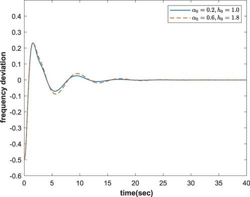
B. Simulation verification

For purpose of validating the accuracy of our theoretical results, we utilize MATLAB/Simulink for simulations based on delayed LFC systems with/without considering probability distribution characteristic. In the simulation, the load fluctuation is chosen as $\omega \left(t\right)=0.1pu$. Based on the different conditions listed in Tables 5 and 7, Figures 2 and 4 present the frequency response trajectory of the system (43(43) $\{\begin{array}{l}\dot{x}\left(t\right)=Ax\left(t\right)+A_{d}x\left(t-h\left(t\right)\right)+B_{\omega }\omega \left(t\right)\\ y\left(t\right)=Cx\left(t\right)\\ x\left(t\right)=\varphi \left(t\right),t\in \left[-h,0\right]\end{array}$(43) ) without considering probability distribution characteristic, then Figures 3 and 5 give the frequency response trajectories of the system (7(7) $\{\begin{array}{rl}\dot{x}\left(t\right)& =Ax\left(t\right)-\alpha \left(t\right)BKCx\left(t-h_1\left(t\right)\right)-\left(1-\alpha \left(t\right)\right)\\ & BKCx\left(t-h_2\left(t\right)\right)+B_{\omega }\omega \left(t\right)\\ y\left(t\right)& =Cx\left(t\right)\\ x\left(t\right)& =\varphi \left(t\right),t\in \left[-h,0\right]\end{array}$(7) ) with considering probability distribution characteristic. It can be seen clearly from the simulation results in Figure 2–5 that all the state variables converge to their equilibrium points, which confirm the veracity of our theoretical results.

Figure 2. State response trajectory with $K_P=0.4$, $K_I=0.4$ by Corollary 3.1.

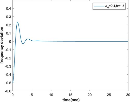
Figure 3. State response trajectories with $K_P=0.4$, $K_I=0.4$ by Theorem 3.1.

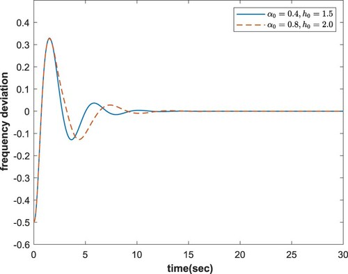
Figure 4. State response trajectory with $K_P=0.2$, $K_I=0.6$ by Corollary 3.1.

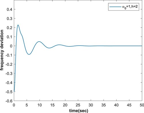
Figure 5. State response trajectories with $K_P=0.2$, $K_I=0.6$ by Theorem 3.1.

5. Conclusion

In this paper, $H_{\mathrm{\infty }}$ performance for PI-type LFC of power systems with random delays have been investigated. By introducing new vectors and delay-dependent matrices, a delay-product-type augmented LKF has been constructed, and a novel extended reciprocally convex matrix inequality combining with Wirtinger-based integral inequality have been employed to tackle with the integral terms effectively, which can utilize more information of time delay and improve the estimation accuracy. According to applied optimal analysis methods, less conservative delay-dependent $H_{\mathrm{\infty }}$ performance and stability criteria have been developed. Finally, two numerical examples have been carried out to illustrate the effectiveness of our theoretical results and the improvement of the proposed methods. In the future, we will consider the influence of other stochastic factors in power systems, construct more reasonable LKF and propose new integral inequalities to further cut down the conservatism of main results.

Acknowledgments

This work was supported in part by the National Natural Science Foundation of China (Grant Nos. 61973105), the Innovation Scientists and Technicians Troop Construction Projects of Henan Province (Grant No. CXTD2016054), Zhongyuan High Level Talents Special Support Plan (Grant No. ZYQR201912031), the Fundamental Research Funds for the Universities of Henan Province (Grant No. NSFRF170501), Innovative Scientists and Technicians Team of Henan Provincial High Education (Grant No. 20IRTSTHN019).

Disclosure statement

No potential conflict of interest was reported by the author(s).

Additional information

Funding

This work was supported in part by the National Natural Science Foundation of China (Grant Nos. 61973105), the Innovation Scientists and Technicians Troop Construction Projects of Henan Province (Grant No. CXTD2016054), Zhongyuan High Level Talents Special Support Plan (Grant No. ZYQR201912031), the Fundamental Research Funds for the Universities of Henan Province (Grant No. NSFRF170501), Innovative Scientists and Technicians Team of Henan Provincial High Education (Grant No. 20IRTSTHN019).

References

- Chen, Y., & Chen, G. (2019). Stability analysis of systems with timevarying delay via a novel Lyapunov functional. IEEE/CAA Journal of Automatica Sinica, 6(4), 1068–1073. https://doi.org/https://doi.org/10.1109/JAS.6570654
- Cheng, Z. H., Yue, D., Hu, S. L., Huang, C. X., Dou, C. X., & Chen, L. (2020). Resilient load frequency control design: DoS attacks against additional control loop. International Journal of Electrical Power & Energy Systems, 115, Article ID: 105496. https://doi.org/https://doi.org/10.1016/j.ijepes.2019.105496
- Fu, C., Wang, C. S., Wang, L. Y., & Shi, D. (2020). An alternative method for mitigating impacts of communication delay on load frequency control. International Journal of Electrical Power & Energy Systems, 119, Article ID: 105924. https://doi.org/https://doi.org/10.1016/j.ijepes.2020.105924
- Jia, F. J., Hu, J., Zhang, P. P., & Chen, D. Y. (2019). Delay-fractioning-based sliding mode control for uncertain nonlinear systems with probabilistic interval delay. In 2019 Chinese control and decision conference (CCDC) (pp. 3145–3150). Institute of Electrical and Electronics Engineers Inc.
- Jiang, L., Yao, W., Wu, Q. H., Wen, J. Y., & Cheng, S. J. (2012). Delay-dependent stability for load frequency control with constant and time-varying delays. IEEE Transactions on Power Systems, 27(2), 932–941. https://doi.org/https://doi.org/10.1109/TPWRS.2011.2172821
- Ko, K. S., Lee, W. I., Park, P. G., & Sung, D. K. (2018). Delays-dependent region partitioning approach for stability criterion of linear systems with multiple time-varying delays. Automatica, 87, 389–394. https://doi.org/https://doi.org/10.1016/j.automatica.2017.09.003
- Lee, W. I., Lee, S. Y., & Park, P. G. (2018). Affine Bessel–Legendre inequality: Application to stability analysis for systems with time-varying delays. Automatica, 93, 535–539. https://doi.org/https://doi.org/10.1016/j.automatica.2018.03.073
- Lee, T. H., & Park, J. H. (2017). A novel Lyapunov functional for stability of time-varying delay systems via matrix-refined-function. Automatica, 80, 239–242. https://doi.org/https://doi.org/10.1016/j.automatica.2017.02.004
- Li, Z. C., Yan, H. C., Zhang, H., Zhan, X. S., & Huang, C. Z. (2019). Improved inequality-based functions approach for stability analysis of time delay system. Automatica, 108. https://doi.org/https://doi.org/10.1016/j.automatica.2019.05.033
- Park, P. G., Ko, J. W., & Jeong, C. (2011). Reciprocally convex approach to stability of systems with time-varying delays. Automatica, 47(1), 235–238. https://doi.org/https://doi.org/10.1016/j.automatica.2010.10.014
- Park, M. J., Kwon, O. M., & Ryu, J. H. (2018). Advanced stability criteria for linear systems with time-varying delays. Journal of the Franklin Institute, 355(1), 520–543. https://doi.org/https://doi.org/10.1016/j.jfranklin.2017.11.029
- Park, P. G., Lee, W. I., & Lee, S. Y. (2015). Auxiliary function-based integral inequalities for quadratic functions and their applications to time-delay systems. Journal of the Franklin Institute, 352(4), 1378–1396. https://doi.org/https://doi.org/10.1016/j.jfranklin.2015.01.004
- Peng, C., Li, J. C., & Fei, M. R. (2017). Resilient event-triggering H∞ load frequency control for multi-area power systems with energy-limited DoS attacks. IEEE Transactions on Power Systems, 32(5), 4110–4118. https://doi.org/https://doi.org/10.1109/TPWRS.2016.2634122
- Peng, C., & Zhang, J. (2016). Delay-distribution-dependent load frequency control of power systems with probabilistic interval delays. IEEE Transactions on Power Systems, 31(4), 3309–3317. https://doi.org/https://doi.org/10.1109/TPWRS.2015.2485272
- Peng, C., Zhang, J., & Yan, H. C. (2018). Adaptive event-triggering H∞ load frequency control for network-based power systems. IEEE Transactions on Industrial Electronics, 65(2), 1685–1694. https://doi.org/https://doi.org/10.1109/TIE.2017.2726965
- Qian, W., Gao, Y. S., & Yang, Y. (2019). Global consensus of multiagent systems with internal delays and communication delays. IEEE Transactions on Systems, Man, and Cybernetics: Systems, 49(10), 1961–1970. https://doi.org/https://doi.org/10.1109/TSMC.6221021
- Qian, W., Li, Y. J., Chen, Y. G., & Liu, W. (2020). L2−L∞ filtering for stochastic delayed systems with randomly occurring nonlinearities and sensor saturation. International Journal of Systems Science, 51(13), 2360–2377. https://doi.org/https://doi.org/10.1080/00207721.2020.1794080
- Qian, W., Li, Y. L., Zhao, Y. J., & Chen, Y. G. (2020). New optimal method for L2−L∞ state estimation of delayed neural networks. Neurocomputing, 415, 258–265. https://doi.org/https://doi.org/10.1016/j.neucom.2020.06.118
- Qian, W., Xing, W. W., & Fei, S. M. (2020). H∞ state estimation for neural networks with general activation function and mixed time-varying delays. IEEE Transactions on Neural Networks and Learning Systems. https://doi.org/https://doi.org/10.1109/TNNLS.2020.3016120
- Sargolzaei, A., Yen, K. K., & Abdelghani, M. N. (2016). Preventing time-delay switch attack on load frequency control in distributed power systems. IEEE Transactions on Smart Grid, 7(2), 1176–1185. https://doi.org/https://doi.org/10.1109/TSG.2015.2503429
- Seuret, A., & Gouaisbaut, F. (2018). Stability of linear systems with time-varying delays using Bessel-Legendre inequalities. IEEE Transactions on Automatic Control, 63(1), 225–232. https://doi.org/https://doi.org/10.1109/TAC.2017.2730485
- Sharma, J., Hote, Y. V., & Prasad, R. (2019). PID controller design for interval load frequency control system with communication time delay. Control Engineering Practice, 89, 154–168. https://doi.org/https://doi.org/10.1016/j.conengprac.2019.05.016
- Shen, C. F., Li, Y., Zhu, X. L., & Duan, W. Y. (2020). Improved stability criteria for linear systems with two additive time-varying delays via a novel Lyapunov functional. Journal of Computational and Applied Mathematics, 363, 312–324. https://doi.org/https://doi.org/10.1016/j.cam.2019.06.010
- Shen, B., Wang, Z. D., & Liu, X. H. (2011). A stochastic sampled-data approach to distributed H∞ filtering in sensor networks. IEEE Transactions on Circuits and Systems I: Regular Papers, 58(9), 2237–2246. https://doi.org/https://doi.org/10.1109/TCSI.2011.2112594
- Singh, V. P., Kishor, N., & Samuel, P. (2016). Load frequency control with communication topology changes in smart grid. IEEE Transactions on Industrial Informatics, 12(5), 1943–1952. https://doi.org/https://doi.org/10.1109/TII.2016.2574242
- Wen, S. P., Yu, X. H., Zeng, Z. G., & Wang, J. J. (2016). Event-triggering load frequency control for multiarea power systems with communication delays. IEEE Transactions on Industrial Electronics, 63(2), 1308–1317. https://doi.org/https://doi.org/10.1109/TIE.41
- Xiong, L. Y., Li, H., & Wang, J. (2018). LMI based robust load frequency control for time delayed power system via delay margin estimation. International Journal of Electrical Power & Energy Systems, 100, 91–103. https://doi.org/https://doi.org/10.1016/j.ijepes.2018.02.027
- Yan, Z. M., & Xu, Y. (2019). Data-driven load frequency control for stochastic power systems: A deep reinforcement learning method with continuous action search. IEEE Transactions on Power Systems, 34(2), 1653–1656. https://doi.org/https://doi.org/10.1109/TPWRS.59
- Zeng, H. B., He, Y., Wu, M., & She, J. H. (2015). Free-matrix-based integral inequality for stability analysis of systems with time-varying delay. IEEE Transactions on Automatic Control, 60(10), 2768–2772. https://doi.org/https://doi.org/10.1109/TAC.2015.2404271
- Zeng, H. B., Liu, X. G., & Wang, W. (2019). A generalized free-matrix-based integral inequality for stability analysis of time-varying delay systems. Applied Mathematics and Computation, 354, 1–8. https://doi.org/https://doi.org/10.1016/j.amc.2019.02.009
- Zhang, C. K., He, Y., Jiang, L., Wang, Q. G., & Wu, M. (2017). Stability analysis of discrete-time neural networks with time-varying delay via an extended reciprocally convex matrix inequality. IEEE Transactions on Cybernetics, 47(10), 3040–3049. https://doi.org/https://doi.org/10.1109/TCYB.2017.2665683
- Zhang, C. K., He, Y., Jiang, L., Wu, M., & Wang, Q. G. (2017). An extended reciprocally convex matrix inequality for stability analysis of systems with time-varying delay. Automatica, 85, 481–485. https://doi.org/https://doi.org/10.1016/j.automatica.2017.07.056
- Zhang, C. K., Jiang, L., Wu, Q. H., He, Y., & Wu, M. (2013). Further results on delay-dependent stability of multi-area load frequency control. IEEE Transactions on Power Systems, 28(4), 4465–4474. https://doi.org/https://doi.org/10.1109/TPWRS.59
- Zhang, H., Liu, J., & Xu, S. Y. (2020). H-infinity load frequency control of networked power systems via an event-triggered scheme. IEEE Transactions on Industrial Electronics, 67(8), 7104–7113. https://doi.org/https://doi.org/10.1109/TIE.41
- Zhang, R. M., Zeng, D. Q., Park, J. H., Zhong, S. M., Liu, Y. J., & Zhou, X. (2019). New approaches to stability analysis for time-varying delay systems. Journal of the Franklin Institute, 356(7), 4174–4189. https://doi.org/https://doi.org/10.1016/j.jfranklin.2019.02.029