Partial-nodes-based state estimation for linear complex networks with randomly occurring sensor delay and stochastic coupling strength

Abstract

This paper is concerned with the partial-nodes-based state estimation (PNBSE) problem for a class of time-varying complex networks with randomly occurring sensor delay (ROSD) and stochastic coupling strength (SCS). We assume that only partial outputs of nodes can be measured and utilized in the estimation algorithm design. The ROSD is expressed by a set of Bernoulli distributed random variables and the occurrence probabilities are certain. Moreover, the SCS is represented by a set of random variables which obeys the uniform distribution. The aim of this paper is to design a recursive state estimator based on the framework of the Kalman filter, where the optimization problem of the upper bound of the estimation error covariance (EEC) is discussed by employing the variance-constrained method. It can be seen that the gain matrix of each node can be obtained by solving two Riccati-like difference equations. In addition, the performance of the PNBSE method is characterized by discussing the relationship between the occurrence probabilities of ROSD and the upper bound of the EEC, where the related mathematical proof is provided. Finally, some simulations are given to show the validity and correctness of the presented PNBSE approach.

Keywords:

• Complex networks
• partial-nodes-based state estimation
• stochastic coupling strength
• randomly occurring sensor delay
• monotonicity analysis

1. Introduction

Complex networks have attracted increasing attention in different fields of scientific research because of their extensive applications, such as World Wide Web, biological networks, power grids, social interactions (Baran & Rzysko, 2020; Chen et al., 2019; Ding et al., 2019; Hu, Wang, et al., 2020). Generally, the information that we can measure only reflect the external characteristics of the systems. But, the behaviours of the systems need to be described by the internal states, which can not be directly measured (Zou et al., 2019, 2020). To better understand the characteristic of the complex networks, the state estimation scheme proposes an effective method to estimate the internal states based on available measurements (W. Li et al., 2017b, 2017c, 2018). In recent years, the problems of synchronization and state estimation have become two important concerns, especially in the analysis of the complex networks (Hu et al., 2016; Hu, Wang, et al., 2020; Wen et al., 2018; Wu et al., 2018). Because the presented state estimation methods not only help to understand the internal structure of complex networks, but also propose the possibility for the coordination utilization of the information of the adjacent nodes. Special attention has been paid to the state estimation problems for complex networks.

Compared with the state estimation for the isolated node, the state estimation problem of complex networks has more research challenges because of the coupling characteristic among different nodes (W. Li et al., 2017a). Generally speaking, the coupling characteristics of complex networks include two aspects, i.e. the outer coupling between two distinct nodes and the inner coupling inside one node only (Hou et al., 2020). In the years, a large number of research results have been obtained based on the assumption that the systems have constant coupling strength. However, it should be pointed out that the coupling strength might be stochastic due to the environmental factors or other reasons. The stochastic coupling strength (SCS) in the complex networks not only increases the dynamical complexity of the networks, but also affects the estimation method performance (Gao et al., 2020). Therefore, the study on the different type couplings among the nodes of complex networks has always been a highly concerned research topic. For example, in Zhang et al. (2019) and Jia et al. (2020), some recursive state estimation methods have been proposed for time-varying dynamical systems with random inner coupling, where the random inner coupling is characterized by multiplicative noise. On the other hand, a recursive state estimation has been designed for complex networks with SCS based on extended Kalman filtering method in W. Li et al. (2017b), where the SCS has been depicted by a set of uniformly distributed random variables with non-negative mean. In addition, in Hu, Liu, et al. (2020), by fully utilizing the event-based communication mechanism, a new robust state estimation algorithm has been proposed for a class of time-varying dynamical networks with random sensor delays and SCS, where both the impacts of random sensor delays and the limitations of the communication resources have been handled simultaneously. In order to further model the complex networks and observe the dynamical behaviours, it is more significant to design a new state estimation strategy for complex networks with SCS, where additional efforts should be made to examine and compensate the SCS.

As it is well known, the core idea of the state estimation problem is to estimate the true states of the systems by accessible measurement outputs (Shen et al., 2020). However, it is generally difficult or expensive to obtain all measurements from every node due to a variety of reasons such as a failure in the measurement, intermittent sensor failures and the loss of some collected data (Liang et al., 2009; D. Liu et al., 2018). Therefore, it is necessary to estimate the states of the systems based on available measurements and ensure certain performance requirements. In recent years, the problem of partial-nodes-based state estimation (PNBSE) has attracted increasing attention since such a problem can be commonly found in the engineering reality, especially for the systems with a great number of coupling nodes (J. Li et al., 2020; Y. Liu, Wang, Yuan, et al., 2019). In fact, the salient feature of PNBSE problem is that the solvability of connectivity degree of networks plays an essential role in its feasibility (Hou et al., 2020). To mention a few, a PNB information fusion method has been exploited in Y. Liu, Wang, Ma, et al. (2019) for stochastic complex networks with discrete-time delay for the first time. In the same way, the problem of PNBSE has been handled in Y. Liu et al. (2018) for a class of continuous-time systems with unbounded distributed delays and energy-bounded measurement noises. So far, there is little literature on PNBSE for complex networks, not to mention the time-varying complex networks undergoing the network transmission. To sum up, the study of PNBSE problem meets more challenges on account of the fact that it is quite difficult to estimate the real states of the whole networks via partial/incomplete node's measurements, which constitutes one motivation of this paper.

The time-delays might affect the performance of systems and even destroy system's stability because of many reasons such as environmental interferences, random congestion of network transmissions, the sensor temporal failures, constrained communication bandwidth and the finite speed of signal transmission for the communication links (Hu, Cui, et al., 2020; Hu et al., 2019; L. Wang et al., 2016). For instance, under the random communication protocol, a resilient state estimation method has been provided in Hu et al. (2019) for discrete nonlinear complex networks with constant time-delays. Moreover, new sufficient conditions have been given to ensure the exponential mean-square boundedness of the estimation error. In addition to the state-delay, the phenomenon of the sensor delay unavoidably exists in the complex networks (Hu, Liu, et al., 2020). In the past years, a great number of literatures suppose that the time-delays are time-invariant. Nonetheless, the time-delays might occur randomly way in practical application and the existence of randomly occurring sensor delays (ROSD) should be considered in complex networks equipped with a large number of nodes (Z. Wang et al., 2004). Therefore, this paper makes one of the first attempts to design the PNBSE scheme for time-varying complex networks, where the SCS, ROSD and time-varying parameter characteristic are taken into account simultaneously. Compared with existing state estimation methods via the all node's measurements, the addressed PNBSE problem lacks the complete node's measurements, thus the satisfactory estimation performance might not be guaranteed. Accordingly, the major advantage is that an effective yet easy-to-implement estimation way should be proposed on the premise of the partial node's measurements.

In this paper, the main aim is to present a PNBSE method for a class of discrete-time complex networks with SCS and ROSD. The phenomenon of SCS is characterized by a set of random variables obeying the uniform distribution with non-negative mean and the ROSD is modelled by the Bernoulli distributed random variables. To be specific, a minimized upper bound matrix of the estimation error covariance (EEC) is established for addressed complex networks by the variance-constrained approach, and the gain matrix of each node can be obtained by minimizing the trace of the upper bound matrix. There are several difficulties in handling the PNBSE problem: (1) How to discuss the effects from the SCS, ROSD and incomplete measurement information onto the estimation performance comprehensively? (2) How to use the measurements of partial nodes to estimate the real states of entire networks and ensure satisfactory estimation accuracy? (3) How to characterize the influences of estimation performance under ROSD with different probabilities rigorously. To answer the above three questions, the main contributions of this paper are summarized from three aspects. (i) A new two-step PNB state estimator is designed, which can effectively estimate the states of whole networks even though only measurements of partial nodes can be obtained. (ii) By considering the statistical information of SCS and ROSD, a locally optimal state estimation algorithm is presented for considered stochastic complex networks subject to time-varying parameter characteristics. In particular, the expression form of the estimator gain is given. It should be mentioned that the new algorithm can reduce the computation burden without resorting the state augmentation idea and it is capable of online applications due to its recursive feature. (iii) A rigorous theoretical proof is presented to show the monotonicity between the upper bound matrix of EEC and the occurrence probabilities of ROSD, which is utilized to reflect the estimation method performance and provides certain reference for corresponding discussions.

Notations

Throughout this paper, ${\mathbb{R}}^n$ represents n-dimensional Euclidean space. $A^T$, $A^{-1}$, $\mathrm{tr}(A)$ stand for the transposition of A, the inverse matrix of A and the trace of A, respectively. I is the identity matrix with appropriate dimension. $\mathrm{diag}\{\cdot \}$ denotes a block-diagonal matrix. The symbol A>B $(A\ge B)$ means that A−B is positive definite (positive semidefinite), where A and B are symmetric matrices. $\mathbb{E}\{\cdot \}$ stands for the mathematical expectation operator. $\mathrm{Prob}\{\cdot \}$ denotes the occurrence probability of the event ‘·’. $\mathrm{Var}\{\cdot \}$ represents the variance of the event ‘·’.

2. Problem statement

Consider the following discrete-time complex networks with SCS and ROSD: (1) $\begin{array}{rl}{x}_{i,k+1}& =A_{i,k}{x}_{i,k}+\sum _{j=1}^N{w}_{ij,k}\mathrm{\Gamma }{x}_{j,k}\\ & +B_{i,k}{\omega }_{i,k},i=1,2,\dots ,N,\end{array}$(1) (2) $\begin{array}{rl}{y}_{i,k}& ={\gamma }_{i,k}{C}_{i,k}{x}_{i,k}+(1-{\gamma }_{i,k})C_{i,k}{x}_{i,k-d}\\ & +{\nu }_{i,k},i=1,2,\dots ,l,\end{array}$(2) where $x_{i,k}\in {\mathbb{R}}^n$ denotes the state vector of the ith node and $y_{i,k}\in {\mathbb{R}}^m$ is the measurement vector of the ith node. N is the node number of the complex networks. $l\le N$ is the node number, in which the observation measurements can be obtained. Γ is a known inner coupling matrix. The random variables ${\gamma }_{i,k}\in \mathbb{R}$ obey the Bernoulli distribution describing the ROSD. d denotes the time delay with constant value. The initial state $x_{i,0}$ has the mean ${\overline{x}}_{i,0}$ and covariance $P_{i,0}$. The process noise ${\omega }_{i,k}$ and the measurement noise ${\nu }_{i,k}$ are zero-mean Gaussian white noises with covariance matrices $Q_{i,k}>0$ and $R_{i,k}>0$, respectively. $A_{i,k}$, $B_{i,k}$ and $C_{i,k}$ are known constant matrices. We assume that ${\omega }_{i,k}$, ${\nu }_{i,k}$, $w_{ij,k}$, ${\gamma }_{i,k}$ and $x_{i,0}$ are mutually independent throughout the paper.

Notice that the random variables $w_{ij,k}$ obey the uniform distribution over the domain $[a_{ij},b_{ij}]$, which characterize the phenomenon of SCS. Accordingly, the mean and variance can be given by $\begin{array}{rl}\mathbb{E}\left\{w_{ij,k}\right\}& ={\overline{w}}_{ij}=\frac{a_{ij}+b_{ij}}{2},\\ \mathrm{Var}\left\{w_{ij,k}\right\}& ={\sigma }_{ij}=\frac{(b_{ij}-a_{ij}{)}^2}{12}.\end{array}$Moreover, the phenomenon of ROSD is modelled by a set of random variables ${\gamma }_{i,k}$ satisfying the Bernoulli distribution with (3) $\begin{array}{rl}\mathrm{Prob}\{{\gamma }_{i,k}=1\}& =\mathbb{E}\left\{{\gamma }_{i,k}\right\}={\overline{\gamma }}_{i,k},\end{array}$(3) (4) $\begin{array}{rl}\mathrm{Prob}\{{\gamma }_{i,k}=0\}& =1-{\overline{\gamma }}_{i,k},\end{array}$(4) where ${\overline{\gamma }}_{i,k}\in \mathbb{R}$ is a known constant. The variance can be expressed as (5) ${\vartheta }_{i,k}=\mathbb{E}\{({\gamma }_{i,k}-{\overline{\gamma }}_{i,k}{)}^2\}=(1-{\overline{\gamma }}_{i,k}){\overline{\gamma }}_{i,k}.$(5)

Remark 2.1

In the existing literature, the scholars commonly assume that the coupling strength between the nodes is a constant (S. Liu et al., 2016). However, the coupling strength might change in a random way especially in the networked environment. For example, the network nodes are distributed in different circumstances, where the communications among the nodes are connected by the network. Thus, the coupling strength might randomly vary accompanying with the environment changes. As such, the phenomenon of SCS is considered and modelled by the uniform distribution over the domain $[a_{ij},b_{ij}]$ to better cater the engineering reality. Owing to the occurrence of the SCS, many unexpected difficulties should be handled in analyzing the dynamical behaviours of the complex networks. For instance, (i) the SCS increases the complexity of the networks; (ii) the accuracy of estimation method might be affected if the phenomenon handled improperly; and (iii) more coupling terms are involved during the estimator design. For this case, the SCS should be analyzed comprehensively and the available information should be utilized properly to deal with the effects of SCS during the state estimator design.

For the ith node, we design the following PNB state estimator for system (1(1) $\begin{array}{rl}{x}_{i,k+1}& =A_{i,k}{x}_{i,k}+\sum _{j=1}^N{w}_{ij,k}\mathrm{\Gamma }{x}_{j,k}\\ & +B_{i,k}{\omega }_{i,k},i=1,2,\dots ,N,\end{array}$(1) ) and (2(2) $\begin{array}{rl}{y}_{i,k}& ={\gamma }_{i,k}{C}_{i,k}{x}_{i,k}+(1-{\gamma }_{i,k})C_{i,k}{x}_{i,k-d}\\ & +{\nu }_{i,k},i=1,2,\dots ,l,\end{array}$(2) ) based on the structure of the Kalman filter: (6) $\begin{array}{rl}{\hat{x}}_{i,k+1|k}& =A_{i,k}{\hat{x}}_{i,k|k}+\sum _{j=1}^N{\overline{w}}_{ij}\mathrm{\Gamma }{\hat{x}}_{j,k|k},\end{array}$(6) (7) $\begin{array}{rl}{\hat{x}}_{i,k+1|k+1}& ={\hat{x}}_{i,k+1|k}+K_{i,k+1}[y_{i,k+1}-{\overline{\gamma }}_{i,k+1}{C}_{i,k+1}\\ & \times {\hat{x}}_{i,k+1|k}-(1-{\overline{\gamma }}_{i,k+1})C_{i,k+1}\\ & \times {\hat{x}}_{i,k+1-d|k+1-d}],i=1,2,\dots ,l,\\ {\hat{x}}_{i,k+1|k+1}& ={\hat{x}}_{i,k+1|k},i=l+1,\dots ,N,\end{array}$(7) where ${\hat{x}}_{i,k+1|k}$ is the prediction for state $x_{i,k}$ of the ith node at time k and ${\hat{x}}_{k+1|k+1}$ is the estimation for state $x_{i,k}$ of the ith node at time k + 1, and $K_{i,k+1}$ is the estimator parameter matrix to be determined at time step k + 1.

Remark 2.2

For general complex networks, the measurement loss may exist during the signal transmissions because of the limited bandwidth of transmission channels and the interference of external environment. On the other hand, note that the complex networks have a large number of nodes generally. However, it is costly or even impossible to obtain the outputs of all nodes for the systems as mentioned in Y. Liu, Wang, Yuan, et al. (2019). Hence, there is an urgent requirement to propose proper way to deal with the state estimation issue for complex networks based on partial node's measurements. Accordingly, we propose a PNB state estimator for the complex networks with N nodes in (6(6) $\begin{array}{rl}{\hat{x}}_{i,k+1|k}& =A_{i,k}{\hat{x}}_{i,k|k}+\sum _{j=1}^N{\overline{w}}_{ij}\mathrm{\Gamma }{\hat{x}}_{j,k|k},\end{array}$(6) ) and (7(7) $\begin{array}{rl}{\hat{x}}_{i,k+1|k+1}& ={\hat{x}}_{i,k+1|k}+K_{i,k+1}[y_{i,k+1}-{\overline{\gamma }}_{i,k+1}{C}_{i,k+1}\\ & \times {\hat{x}}_{i,k+1|k}-(1-{\overline{\gamma }}_{i,k+1})C_{i,k+1}\\ & \times {\hat{x}}_{i,k+1-d|k+1-d}],i=1,2,\dots ,l,\\ {\hat{x}}_{i,k+1|k+1}& ={\hat{x}}_{i,k+1|k},i=l+1,\dots ,N,\end{array}$(7) ). In order to overcome the difficulties caused by unavailability of partial node's measurements, an alternative way is adopted and the two-step estimation scheme based on the Kalman filter is given. To be more specific, the states of the first l nodes are estimated via the corresponding node's measurements and the state estimations of the latter N−l nodes are obtained by the prediction estimation information, where the estimation way without the node's measurements is similar to the idea in the predictive control theory. In other words, the state estimations of the whole networks can be obtained by developing the PNBSE method when the number of available node's measurements is less than the total number of nodes, which is indeed helpful for handling the state estimation problems of complex networks with incomplete node's measurements and contributes the major motivation of the conducted topic.

Subsequently, the prediction error, the estimation error and the corresponding covariances are defined as follows: (8) $\begin{array}{rl}{e}_{i,k+1|k}& =x_{i,k+1}-{\hat{x}}_{i,k+1|k},\end{array}$(8) (9) $\begin{array}{rl}{e}_{i,k+1|k+1}& =x_{i,k+1}-{\hat{x}}_{i,k+1|k+1},\end{array}$(9) (10) $\begin{array}{rl}{P}_{i,k+1|k}& =\mathbb{E}\left\{e_{i,k+1|k}{e}_{i,k+1|k}^T\right\},\end{array}$(10) (11) $\begin{array}{rl}{P}_{i,k+1|k+1}& =\mathbb{E}\left\{e_{i,k+1|k+1}{e}_{i,k+1|k+1}^T\right\}.\end{array}$(11) The aim of this paper is to design a PNB state estimator described by (6(6) $\begin{array}{rl}{\hat{x}}_{i,k+1|k}& =A_{i,k}{\hat{x}}_{i,k|k}+\sum _{j=1}^N{\overline{w}}_{ij}\mathrm{\Gamma }{\hat{x}}_{j,k|k},\end{array}$(6) ) and (7(7) $\begin{array}{rl}{\hat{x}}_{i,k+1|k+1}& ={\hat{x}}_{i,k+1|k}+K_{i,k+1}[y_{i,k+1}-{\overline{\gamma }}_{i,k+1}{C}_{i,k+1}\\ & \times {\hat{x}}_{i,k+1|k}-(1-{\overline{\gamma }}_{i,k+1})C_{i,k+1}\\ & \times {\hat{x}}_{i,k+1-d|k+1-d}],i=1,2,\dots ,l,\\ {\hat{x}}_{i,k+1|k+1}& ={\hat{x}}_{i,k+1|k},i=l+1,\dots ,N,\end{array}$(7) ) such that (i) a sequence of positive-definite matrices ${\mathrm{\Sigma }}_{i,k+1|k+1}$ satisfying $P_{i,k+1|k+1}\le {\mathrm{\Sigma }}_{i,k+1|k+1};$(ii) the gain matrix $K_{i,k+1}$ is determined to minimize the trace of the upper bound matrix ${\mathrm{\Sigma }}_{i,k+1|k+1}$ at each time instant; and (iii) the algorithm performance of the PNBSE is discussed.

3. Main results

In this section, we need to find the upper bound of the EEC firstly and derive the gain matrix of each node by minimizing the trace of the upper bound matrix. Before designing the gain matrix, the following lemmas are introduced.

Lemma 3.1

Kluge et al., 2010

For real vectors $x\in \mathbb{R}$ and $y\in \mathbb{R}$ of the appropriate dimensions, one has (12) $x{y}^T+y{x}^T\le \eta x{x}^T+{\eta }^{-1}y{y}^T,$(12) where η is a positive constant.

Lemma 3.2

Theodor & Shaked, 1996

For $0\le k<n$, suppose that $A=A^T>0$. Let $\phi (\cdot ):{\mathbb{R}}^{n\times n}\to {\mathbb{R}}^{n\times n}$ and $\varphi (\cdot ):{\mathbb{R}}^{n\times n}\to {\mathbb{R}}^{n\times n}$ be two sequences of matrix functions such that (13) ${\phi }_k(A)={\phi }_k(A^T),{\varphi }_k(A)={\varphi }_k(A^T).$(13) If there exists a matrix $B=B^T>A$ such that (14) ${\phi }_k(B)\ge {\phi }_k(A),{\varphi }_k(B)={\phi }_k(B),$(14) then the solutions $X_k$ and $Y_k$ to the following difference equations (15) $X_k={\phi }_k(X_{k-1}),Y_k={\varphi }_k(X_{k-1}),X_0=Y_0>0,$(15) satisfy $X_k\le Y_k$.

Lemma 3.3

Hu et al., 2016

For real matrices M, N, X with appropriate dimensions and symmetric matrix P, the following equations hold (16) $\begin{array}{r}\begin{array}{rl}& \frac{\mathrm{\partial }\mathrm{tr}[(MXN)P(MXN{)}^T]}{\mathrm{\partial }X}=2M^{T}MXNP{N}^T,\\ & \frac{\mathrm{\partial }\mathrm{tr}(MXN)}{\mathrm{\partial }X}=M^T{N}^T,\frac{\mathrm{\partial }\mathrm{tr}(M{X}^{T}N)}{\mathrm{\partial }X}=NM,\\ & \frac{\mathrm{\partial }\mathrm{tr}(XA{X}^T)}{\mathrm{\partial }X}=2XA.\end{array}\end{array}$(16)

Based on the definitions in (8(8) $\begin{array}{rl}{e}_{i,k+1|k}& =x_{i,k+1}-{\hat{x}}_{i,k+1|k},\end{array}$(8) )–(11(11) $\begin{array}{rl}{P}_{i,k+1|k+1}& =\mathbb{E}\left\{e_{i,k+1|k+1}{e}_{i,k+1|k+1}^T\right\}.\end{array}$(11) ), we present the following theorem, where both an optimized upper bound ${\mathrm{\Sigma }}_{i,k+1|k+1}$ of the EEC $P_{i,k+1|k+1}$ and the corresponding estimator gain matrix $K_{i,k+1}$ are presented.

Theorem 3.1

For given positive scalars ${\eta }_i$ $(i=1,2,3,4)$, if the following two Riccati-like difference equations (17) $\begin{array}{rl}& {\mathrm{\Sigma }}_{i,k+1|k}\\ & =(1+{\overline{w}}_i)A_{i,k}{\mathrm{\Sigma }}_{i,k|k}{A}_{i,k}^T+B_{i,k}{Q}_{i,k}{B}_{i,k}^T\\ & +\sum _{j=1}^l(2{\sigma }_{ij}+{\overline{w}}_i{\overline{w}}_{ij}+{\overline{w}}_{ij})\mathrm{\Gamma }{\mathrm{\Sigma }}_{j,k|k}{\mathrm{\Gamma }}^T\\ & +\sum _{j=l+1}^N(2{\sigma }_{ij}+{\overline{w}}_i{\overline{w}}_{ij}+{\overline{w}}_{ij})\mathrm{\Gamma }{\mathrm{\Sigma }}_{j,k|k}{\mathrm{\Gamma }}^T\\ & +2\sum _{j=1}^l{\sigma }_{ij}\mathrm{\Gamma }{\hat{x}}_{j,k|k}{\hat{x}}_{j,k|k}^T{\mathrm{\Gamma }}^T\\ & +2\sum _{j=l+1}^N{\sigma }_{ij}\mathrm{\Gamma }{\hat{x}}_{j,k|k}{\hat{x}}_{j,k|k}^T{\mathrm{\Gamma }}^T,\end{array}$(17) (18) $\begin{array}{rl}& {\mathrm{\Sigma }}_{i,k+1|k+1}\\ & =(1+{\eta }_3)[I-{\overline{\gamma }}_{i,k+1}{K}_{i,k+1}{C}_{i,k+1}]{\mathrm{\Sigma }}_{i,k+1|k}[I-{\overline{\gamma }}_{i,k+1}\\ & \times K_{i,k+1}{C}_{i,k+1}{]}^T+(1+{\eta }_3^{-1})(1-{\overline{\gamma }}_{i,k+1}{)}^2{K}_{i,k+1}\\ & \times C_{i,k+1}{\mathrm{\Sigma }}_{i,k+1-d|k+1-d}{C}_{i,k+1}^T{K}_{i,k+1}^T+(1+{\eta }_4)\\ & \times {\overline{\gamma }}_{i,k+1}(1-{\overline{\gamma }}_{i,k+1})K_{i,k+1}{C}_{i,k+1}{\overline{\mathrm{\Phi }}}_{i,k+1|k+1}\\ & \times C_{i,k+1}^T{K}_{i,k+1}^T+(1+{\eta }_4^{-1}){\overline{\gamma }}_{i,k+1}(1-{\overline{\gamma }}_{i,k+1})\\ & \times K_{i,k+1}{C}_{i,k+1}{\overline{\mathrm{\Phi }}}_{i,k+1-d|k+1-d}{C}_{i,k+1}^T{K}_{i,k+1}^T\\ & +K_{i,k+1}{R}_{i,k+1}{K}_{i,k+1}^T,i=1,2,\dots ,l,\\ & {\mathrm{\Sigma }}_{i,k+1|k+1}={\mathrm{\Sigma }}_{i,k+1|k},i=l+1,\dots ,N,\end{array}$(18) have positive-definite solutions ${\mathrm{\Sigma }}_{i,k+1|k}$ and ${\mathrm{\Sigma }}_{i,k+1|k+1}$, then we have $P_{i,k+1|k+1}\le {\mathrm{\Sigma }}_{i,k+1|k+1}.$Moreover, if the estimator gain matrix is given by (19) $\begin{array}{rl}& K_{i,k+1}\\ & =(1+{\eta }_3){\overline{\gamma }}_{i,k+1}{\mathrm{\Sigma }}_{i,k+1|k}{C}_{i,k+1}^T\{(1+{\eta }_3){\overline{\gamma }}_{i,k+1}^2{C}_{i,k+1}\\ & \times {\mathrm{\Sigma }}_{i,k+1|k}{C}_{i,k+1}^T+(1+{\eta }_3^{-1})(1-{\overline{\gamma }}_{i,k+1}{)}^2{C}_{i,k+1}\\ & \times {\mathrm{\Sigma }}_{i,k+1-d|k+1-d}{C}_{i,k+1}^T+(1+{\eta }_4){\overline{\gamma }}_{i,k+1}\\ & \times (1-{\overline{\gamma }}_{i,k+1})C_{i,k+1}{\overline{\mathrm{\Phi }}}_{i,k+1|k+1}{C}_{i,k+1}^T\\ & +(1+{\eta }_4^{-1}){\overline{\gamma }}_{i,k+1}(1-{\overline{\gamma }}_{i,k+1})C_{i,k+1}\\ & \times {\overline{\mathrm{\Phi }}}_{i,k+1-d|k+1-d}{C}_{i,k+1}^T+R_{i,k+1}{\}}^{-1},\end{array}$(19) then $\mathrm{tr}({\mathrm{\Sigma }}_{i,k+1|k+1})$ can be minimized.

Proof.

Firstly, we can obtain the prediction error by substituting (1(1) $\begin{array}{rl}{x}_{i,k+1}& =A_{i,k}{x}_{i,k}+\sum _{j=1}^N{w}_{ij,k}\mathrm{\Gamma }{x}_{j,k}\\ & +B_{i,k}{\omega }_{i,k},i=1,2,\dots ,N,\end{array}$(1) ) and (6(6) $\begin{array}{rl}{\hat{x}}_{i,k+1|k}& =A_{i,k}{\hat{x}}_{i,k|k}+\sum _{j=1}^N{\overline{w}}_{ij}\mathrm{\Gamma }{\hat{x}}_{j,k|k},\end{array}$(6) ) into (8(8) $\begin{array}{rl}{e}_{i,k+1|k}& =x_{i,k+1}-{\hat{x}}_{i,k+1|k},\end{array}$(8) ) (20) $\begin{array}{rlrl}& e_{i,k+1|k}& =A_{i,k}{e}_{i,k|k}+\sum _{j=1}^N(w_{ij,k}-{\overline{w}}_{ij})\mathrm{\Gamma }{x}_{j,k}+\sum _{j=1}^l{\overline{w}}_{ij}\mathrm{\Gamma }{e}_{j,k|k}& +\sum _{j=l+1}^N{\overline{w}}_{ij}\mathrm{\Gamma }{e}_{j,k|k}+B_{i,k}{\omega }_{i,k}.\end{array}$(20) Then, the prediction error covariance can be calculated based on (10(10) $\begin{array}{rl}{P}_{i,k+1|k}& =\mathbb{E}\left\{e_{i,k+1|k}{e}_{i,k+1|k}^T\right\},\end{array}$(10) ) and (20(20) $\begin{array}{rlrl}& e_{i,k+1|k}& =A_{i,k}{e}_{i,k|k}+\sum _{j=1}^N(w_{ij,k}-{\overline{w}}_{ij})\mathrm{\Gamma }{x}_{j,k}+\sum _{j=1}^l{\overline{w}}_{ij}\mathrm{\Gamma }{e}_{j,k|k}& +\sum _{j=l+1}^N{\overline{w}}_{ij}\mathrm{\Gamma }{e}_{j,k|k}+B_{i,k}{\omega }_{i,k}.\end{array}$(20) ): (21) $\begin{array}{rlrlrlrlr}& P_{i,k+1|k}& =A_{i,k}{P}_{i,k|k}{A}_{i,k}^T+\sum _{j=1}^N{\sigma }_{ij}\mathbb{E}\{\mathrm{\Gamma }{x}_{j,k}{x}_{j,k}^T{\mathrm{\Gamma }}^T\}& +\sum _{j=1}^l\sum _{s=1}^l{\overline{w}}_{ij}{\overline{w}}_{is}\mathbb{E}\{\mathrm{\Gamma }{e}_{j,k|k}{e}_{s,k|k}^T{\mathrm{\Gamma }}^T\}& +\sum _{j=l+1}^N\sum _{s=l+1}^N{\overline{w}}_{ij}{\overline{w}}_{is}\mathbb{E}\{\mathrm{\Gamma }{e}_{j,k|k}{e}_{s,k|k}^T{\mathrm{\Gamma }}^T\}& +B_{i,k}{Q}_{i,k}{B}_{i,k}^T+\sum _{j=1}^l{\overline{w}}_{ij}\mathbb{E}\{A_{i,k}{e}_{i,k|k}{e}_{j,k|k}^T{\mathrm{\Gamma }}^T& +\mathrm{\Gamma }{e}_{j,k|k}{e}_{i,k|k}^T{A}_{i,k}^T\}+\sum _{j=l+1}^N{\overline{w}}_{ij}\mathbb{E}\{A_{i,k}{e}_{i,k|k}{e}_{j,k|k}^T{\mathrm{\Gamma }}^T& +\mathrm{\Gamma }{e}_{j,k|k}{e}_{i,k|k}^T{A}_{i,k}^T\}+\sum _{j=1}^l\sum _{s=l+1}^N{\overline{w}}_{ij}{\overline{w}}_{is}\mathbb{E}\{\mathrm{\Gamma }{e}_{j,k|k}{e}_{s,k|k}^T{\mathrm{\Gamma }}^T& +\mathrm{\Gamma }{e}_{s,k|k}{e}_{j,k|k}^T{\mathrm{\Gamma }}^T\},\end{array}$(21) where ${\sigma }_{ij}=\mathbb{E}\{(w_{ij,k}-{\overline{w}}_{ij}{)}^2\}$, and $\mathbb{E}\{(w_{ij,k}-{\overline{w}}_{ij})(w_{is,k}-{\overline{w}}_{is})\mathrm{\Gamma }{x}_{j,k}{x}_{s,k}^T{\mathrm{\Gamma }}^T\}=0$, if $j\ne s$.

Notice that $x_{j,k}=e_{j,k|k}+{\hat{x}}_{j,k|k}$, the second term on the right hand side of (21(21) $\begin{array}{rlrlrlrlr}& P_{i,k+1|k}& =A_{i,k}{P}_{i,k|k}{A}_{i,k}^T+\sum _{j=1}^N{\sigma }_{ij}\mathbb{E}\{\mathrm{\Gamma }{x}_{j,k}{x}_{j,k}^T{\mathrm{\Gamma }}^T\}& +\sum _{j=1}^l\sum _{s=1}^l{\overline{w}}_{ij}{\overline{w}}_{is}\mathbb{E}\{\mathrm{\Gamma }{e}_{j,k|k}{e}_{s,k|k}^T{\mathrm{\Gamma }}^T\}& +\sum _{j=l+1}^N\sum _{s=l+1}^N{\overline{w}}_{ij}{\overline{w}}_{is}\mathbb{E}\{\mathrm{\Gamma }{e}_{j,k|k}{e}_{s,k|k}^T{\mathrm{\Gamma }}^T\}& +B_{i,k}{Q}_{i,k}{B}_{i,k}^T+\sum _{j=1}^l{\overline{w}}_{ij}\mathbb{E}\{A_{i,k}{e}_{i,k|k}{e}_{j,k|k}^T{\mathrm{\Gamma }}^T& +\mathrm{\Gamma }{e}_{j,k|k}{e}_{i,k|k}^T{A}_{i,k}^T\}+\sum _{j=l+1}^N{\overline{w}}_{ij}\mathbb{E}\{A_{i,k}{e}_{i,k|k}{e}_{j,k|k}^T{\mathrm{\Gamma }}^T& +\mathrm{\Gamma }{e}_{j,k|k}{e}_{i,k|k}^T{A}_{i,k}^T\}+\sum _{j=1}^l\sum _{s=l+1}^N{\overline{w}}_{ij}{\overline{w}}_{is}\mathbb{E}\{\mathrm{\Gamma }{e}_{j,k|k}{e}_{s,k|k}^T{\mathrm{\Gamma }}^T& +\mathrm{\Gamma }{e}_{s,k|k}{e}_{j,k|k}^T{\mathrm{\Gamma }}^T\},\end{array}$(21) ) is derived as follows: (22) $\begin{array}{rlrl}& \sum _{j=1}^N{\sigma }_{ij}\mathbb{E}\{\mathrm{\Gamma }{x}_{j,k}{x}_{j,k}^T{\mathrm{\Gamma }}^T\}& =\sum _{j=1}^l{\sigma }_{ij}\mathbb{E}\{\mathrm{\Gamma }(e_{j,k|k}+{\hat{x}}_{j,k|k})(e_{j,k|k}+{\hat{x}}_{j,k|k}{)}^T{\mathrm{\Gamma }}^T\}& +\sum _{j=l+1}^N{\sigma }_{ij}\mathbb{E}\{\mathrm{\Gamma }(e_{j,k|k}+{\hat{x}}_{j,k|k})(e_{j,k|k}+{\hat{x}}_{j,k|k}{)}^T{\mathrm{\Gamma }}^T\}\\ & \le 2\sum _{j=1}^l{\sigma }_{ij}\mathrm{\Gamma }{\hat{x}}_{j,k|k}{\hat{x}}_{j,k|k}^T{\mathrm{\Gamma }}^T+2\sum _{j=l+1}^N{\sigma }_{ij}\mathrm{\Gamma }{\hat{x}}_{j,k|k}{\hat{x}}_{j,k|k}^T{\mathrm{\Gamma }}^T\\ & +2\sum _{j=1}^l{\sigma }_{ij}\mathrm{\Gamma }{P}_{j,k|k}{\mathrm{\Gamma }}^T+2\sum _{j=l+1}^N{\sigma }_{ij}\mathrm{\Gamma }{P}_{j,k|k}{\mathrm{\Gamma }}^T.\end{array}$(22) By using Lemma 3.1, the third and the fourth terms on the right hand side of (21(21) $\begin{array}{rlrlrlrlr}& P_{i,k+1|k}& =A_{i,k}{P}_{i,k|k}{A}_{i,k}^T+\sum _{j=1}^N{\sigma }_{ij}\mathbb{E}\{\mathrm{\Gamma }{x}_{j,k}{x}_{j,k}^T{\mathrm{\Gamma }}^T\}& +\sum _{j=1}^l\sum _{s=1}^l{\overline{w}}_{ij}{\overline{w}}_{is}\mathbb{E}\{\mathrm{\Gamma }{e}_{j,k|k}{e}_{s,k|k}^T{\mathrm{\Gamma }}^T\}& +\sum _{j=l+1}^N\sum _{s=l+1}^N{\overline{w}}_{ij}{\overline{w}}_{is}\mathbb{E}\{\mathrm{\Gamma }{e}_{j,k|k}{e}_{s,k|k}^T{\mathrm{\Gamma }}^T\}& +B_{i,k}{Q}_{i,k}{B}_{i,k}^T+\sum _{j=1}^l{\overline{w}}_{ij}\mathbb{E}\{A_{i,k}{e}_{i,k|k}{e}_{j,k|k}^T{\mathrm{\Gamma }}^T& +\mathrm{\Gamma }{e}_{j,k|k}{e}_{i,k|k}^T{A}_{i,k}^T\}+\sum _{j=l+1}^N{\overline{w}}_{ij}\mathbb{E}\{A_{i,k}{e}_{i,k|k}{e}_{j,k|k}^T{\mathrm{\Gamma }}^T& +\mathrm{\Gamma }{e}_{j,k|k}{e}_{i,k|k}^T{A}_{i,k}^T\}+\sum _{j=1}^l\sum _{s=l+1}^N{\overline{w}}_{ij}{\overline{w}}_{is}\mathbb{E}\{\mathrm{\Gamma }{e}_{j,k|k}{e}_{s,k|k}^T{\mathrm{\Gamma }}^T& +\mathrm{\Gamma }{e}_{s,k|k}{e}_{j,k|k}^T{\mathrm{\Gamma }}^T\},\end{array}$(21) ) can be bounded by: (23) $\begin{array}{rl}& \sum _{j=1}^l\sum _{s=1}^l{\overline{w}}_{ij}{\overline{w}}_{is}\mathbb{E}\{\mathrm{\Gamma }{e}_{j,k|k}{e}_{s,k|k}^T{\mathrm{\Gamma }}^T\}\\ & \le \frac{1}{2}\sum _{j=1}^l\sum _{s=1}^l{\overline{w}}_{ij}{\overline{w}}_{is}\mathbb{E}\{\mathrm{\Gamma }{P}_{j,k|k}{\mathrm{\Gamma }}^T+\mathrm{\Gamma }{P}_{s,k|k}{\mathrm{\Gamma }}^T\}\\ & =\sum _{j=1}^l\left(\sum _{s=1}^l{\overline{w}}_{is}\right){\overline{w}}_{ij}\mathrm{\Gamma }{P}_{j,k|k}{\mathrm{\Gamma }}^T,\end{array}$(23) (24) $\begin{array}{rl}& \sum _{j=l+1}^N\sum _{s=l+1}^N{\overline{w}}_{ij}{\overline{w}}_{is}\mathbb{E}\{\mathrm{\Gamma }{e}_{j,k|k}{e}_{s,k|k}^T{\mathrm{\Gamma }}^T\}\\ & \le \frac{1}{2}\sum _{j=l+1}^N\sum _{s=l+1}^N{\overline{w}}_{ij}{\overline{w}}_{is}\mathbb{E}\{\mathrm{\Gamma }{P}_{j,k|k}{\mathrm{\Gamma }}^T+\mathrm{\Gamma }{P}_{s,k|k}{\mathrm{\Gamma }}^T\}\\ & =\sum _{j=l+1}^N\left(\sum _{s=l+1}^N{\overline{w}}_{is}\right){\overline{w}}_{ij}\mathrm{\Gamma }{P}_{j,k|k}{\mathrm{\Gamma }}^T.\end{array}$(24) Similarly, the sixth, the seventh and the eighth terms on the right hand side of (21(21) $\begin{array}{rlrlrlrlr}& P_{i,k+1|k}& =A_{i,k}{P}_{i,k|k}{A}_{i,k}^T+\sum _{j=1}^N{\sigma }_{ij}\mathbb{E}\{\mathrm{\Gamma }{x}_{j,k}{x}_{j,k}^T{\mathrm{\Gamma }}^T\}& +\sum _{j=1}^l\sum _{s=1}^l{\overline{w}}_{ij}{\overline{w}}_{is}\mathbb{E}\{\mathrm{\Gamma }{e}_{j,k|k}{e}_{s,k|k}^T{\mathrm{\Gamma }}^T\}& +\sum _{j=l+1}^N\sum _{s=l+1}^N{\overline{w}}_{ij}{\overline{w}}_{is}\mathbb{E}\{\mathrm{\Gamma }{e}_{j,k|k}{e}_{s,k|k}^T{\mathrm{\Gamma }}^T\}& +B_{i,k}{Q}_{i,k}{B}_{i,k}^T+\sum _{j=1}^l{\overline{w}}_{ij}\mathbb{E}\{A_{i,k}{e}_{i,k|k}{e}_{j,k|k}^T{\mathrm{\Gamma }}^T& +\mathrm{\Gamma }{e}_{j,k|k}{e}_{i,k|k}^T{A}_{i,k}^T\}+\sum _{j=l+1}^N{\overline{w}}_{ij}\mathbb{E}\{A_{i,k}{e}_{i,k|k}{e}_{j,k|k}^T{\mathrm{\Gamma }}^T& +\mathrm{\Gamma }{e}_{j,k|k}{e}_{i,k|k}^T{A}_{i,k}^T\}+\sum _{j=1}^l\sum _{s=l+1}^N{\overline{w}}_{ij}{\overline{w}}_{is}\mathbb{E}\{\mathrm{\Gamma }{e}_{j,k|k}{e}_{s,k|k}^T{\mathrm{\Gamma }}^T& +\mathrm{\Gamma }{e}_{s,k|k}{e}_{j,k|k}^T{\mathrm{\Gamma }}^T\},\end{array}$(21) ) can be bounded by: (25) $\begin{array}{rl}& \sum _{j=1}^l{\overline{w}}_{ij}\mathbb{E}\{A_{i,k}{e}_{i,k|k}{e}_{j,k|k}^T{\mathrm{\Gamma }}^T+\mathrm{\Gamma }{e}_{j,k|k}{e}_{i,k|k}^T{A}_{i,k}^T\}\\ & \le \sum _{j=1}^l{\overline{w}}_{ij}{A}_{i,k}{P}_{i,k|k}{A}_{i,k}^T+\sum _{j=1}^l{\overline{w}}_{ij}\mathrm{\Gamma }{P}_{j,k|k}{\mathrm{\Gamma }}^T,\end{array}$(25) (26) $\begin{array}{rl}& \sum _{j=l+1}^N{\overline{w}}_{ij}\mathbb{E}\{A_{i,k}{e}_{i,k|k}{e}_{j,k|k}^T{\mathrm{\Gamma }}^T+\mathrm{\Gamma }{e}_{j,k|k}{e}_{i,k|k}^T{A}_{i,k}^T\}\\ & \le \sum _{j=l+1}^N{\overline{w}}_{ij}{A}_{i,k}{P}_{i,k|k}{A}_{i,k}^T+\sum _{j=l+1}^N{\overline{w}}_{ij}\mathrm{\Gamma }{P}_{j,k|k}{\mathrm{\Gamma }}^T,\end{array}$(26) (27) $\begin{array}{rl}& \sum _{j=1}^l\sum _{s=l+1}^N{\overline{w}}_{ij}{\overline{w}}_{is}\mathbb{E}\{\mathrm{\Gamma }{e}_{j,k|k}{e}_{s,k|k}^T{\mathrm{\Gamma }}^T+\mathrm{\Gamma }{e}_{s,k|k}{e}_{j,k|k}^T{\mathrm{\Gamma }}^T\}\\ & \le \sum _{j=1}^l\sum _{s=l+1}^N{\overline{w}}_{ij}{\overline{w}}_{is}\mathrm{\Gamma }{P}_{j,k|k}{\mathrm{\Gamma }}^T\\ & +\sum _{j=1}^l\sum _{s=l+1}^N{\overline{w}}_{ij}{\overline{w}}_{is}\mathrm{\Gamma }{P}_{s,k|k}{\mathrm{\Gamma }}^T.\end{array}$(27) Based on the inequalities mentioned above, combining (22(22) $\begin{array}{rlrl}& \sum _{j=1}^N{\sigma }_{ij}\mathbb{E}\{\mathrm{\Gamma }{x}_{j,k}{x}_{j,k}^T{\mathrm{\Gamma }}^T\}& =\sum _{j=1}^l{\sigma }_{ij}\mathbb{E}\{\mathrm{\Gamma }(e_{j,k|k}+{\hat{x}}_{j,k|k})(e_{j,k|k}+{\hat{x}}_{j,k|k}{)}^T{\mathrm{\Gamma }}^T\}& +\sum _{j=l+1}^N{\sigma }_{ij}\mathbb{E}\{\mathrm{\Gamma }(e_{j,k|k}+{\hat{x}}_{j,k|k})(e_{j,k|k}+{\hat{x}}_{j,k|k}{)}^T{\mathrm{\Gamma }}^T\}\\ & \le 2\sum _{j=1}^l{\sigma }_{ij}\mathrm{\Gamma }{\hat{x}}_{j,k|k}{\hat{x}}_{j,k|k}^T{\mathrm{\Gamma }}^T+2\sum _{j=l+1}^N{\sigma }_{ij}\mathrm{\Gamma }{\hat{x}}_{j,k|k}{\hat{x}}_{j,k|k}^T{\mathrm{\Gamma }}^T\\ & +2\sum _{j=1}^l{\sigma }_{ij}\mathrm{\Gamma }{P}_{j,k|k}{\mathrm{\Gamma }}^T+2\sum _{j=l+1}^N{\sigma }_{ij}\mathrm{\Gamma }{P}_{j,k|k}{\mathrm{\Gamma }}^T.\end{array}$(22) )–(27(27) $\begin{array}{rl}& \sum _{j=1}^l\sum _{s=l+1}^N{\overline{w}}_{ij}{\overline{w}}_{is}\mathbb{E}\{\mathrm{\Gamma }{e}_{j,k|k}{e}_{s,k|k}^T{\mathrm{\Gamma }}^T+\mathrm{\Gamma }{e}_{s,k|k}{e}_{j,k|k}^T{\mathrm{\Gamma }}^T\}\\ & \le \sum _{j=1}^l\sum _{s=l+1}^N{\overline{w}}_{ij}{\overline{w}}_{is}\mathrm{\Gamma }{P}_{j,k|k}{\mathrm{\Gamma }}^T\\ & +\sum _{j=1}^l\sum _{s=l+1}^N{\overline{w}}_{ij}{\overline{w}}_{is}\mathrm{\Gamma }{P}_{s,k|k}{\mathrm{\Gamma }}^T.\end{array}$(27) ) with $P_{i,k+1|k}$, one has (28) $\begin{array}{rl}& P_{i,k+1|k}\\ & \le (1+{\overline{w}}_i)A_{i,k}{P}_{i,k|k}{A}_{i,k}^T+B_{i,k}{Q}_{i,k}{B}_{i,k}^T\\ & +\sum _{j=1}^l(2{\sigma }_{ij}+{\overline{w}}_i{\overline{w}}_{ij}+{\overline{w}}_{ij})\mathrm{\Gamma }{P}_{j,k|k}{\mathrm{\Gamma }}^T\\ & +\sum _{j=l+1}^N(2{\sigma }_{ij}+{\overline{w}}_i{\overline{w}}_{ij}+{\overline{w}}_{ij})\mathrm{\Gamma }{P}_{j,k|k}{\mathrm{\Gamma }}^T\\ & +2\sum _{j=1}^l{\sigma }_{ij}\mathrm{\Gamma }{\hat{x}}_{j,k|k}{\hat{x}}_{j,k|k}^T{\mathrm{\Gamma }}^T\\ & +2\sum _{j=l+1}^N{\sigma }_{ij}\mathrm{\Gamma }{\hat{x}}_{j,k|k}{\hat{x}}_{j,k|k}^T{\mathrm{\Gamma }}^T,\end{array}$(28) where $\sum _{j=1}^N{\overline{w}}_{ij}={\overline{w}}_i$.

Next, we will derive the upper bound matrix for the EEC. To begin, set ${\tilde{\gamma }}_{i,k+1}={\gamma }_{i,k+1}-{\overline{\gamma }}_{i,k+1}$. Then, the estimation error $e_{i,k+1|k+1}$ can be obtained (29) $\begin{array}{rl}{e}_{i,k+1|k+1}& =[I-{\overline{\gamma }}_{i,k+1}{K}_{i,k+1}{C}_{i,k+1}]e_{i,k+1|k}\\ & -(1-{\overline{\gamma }}_{i,k+1})K_{i,k+1}{C}_{i,k+1}{e}_{i,k+1-d|k+1-d}\\ & +{\tilde{\gamma }}_{i,k+1}{K}_{i,k+1}{C}_{i,k+1}{x}_{i,k+1-d}\\ & -{\tilde{\gamma }}_{i,k+1}{K}_{i,k+1}{C}_{i,k+1}{x}_{i,k+1}\\ & -K_{i,k+1}{\nu }_{i,k+1},i=1,2,\dots ,l,\\ e_{i,k+1|k+1}& =e_{i,k+1|k},i=l+1,\dots ,N.\end{array}$(29) Subsequently, the corresponding covariance can be obtained from (29(29) $\begin{array}{rl}{e}_{i,k+1|k+1}& =[I-{\overline{\gamma }}_{i,k+1}{K}_{i,k+1}{C}_{i,k+1}]e_{i,k+1|k}\\ & -(1-{\overline{\gamma }}_{i,k+1})K_{i,k+1}{C}_{i,k+1}{e}_{i,k+1-d|k+1-d}\\ & +{\tilde{\gamma }}_{i,k+1}{K}_{i,k+1}{C}_{i,k+1}{x}_{i,k+1-d}\\ & -{\tilde{\gamma }}_{i,k+1}{K}_{i,k+1}{C}_{i,k+1}{x}_{i,k+1}\\ & -K_{i,k+1}{\nu }_{i,k+1},i=1,2,\dots ,l,\\ e_{i,k+1|k+1}& =e_{i,k+1|k},i=l+1,\dots ,N.\end{array}$(29) ) that (30) $\begin{array}{rl}& P_{i,k+1|k+1}\\ & =[I-{\overline{\gamma }}_{i,k+1}{K}_{i,k+1}{C}_{i,k+1}]P_{i,k+1|k}[I-{\overline{\gamma }}_{i,k+1}{K}_{i,k+1}\\ & \times C_{i,k+1}{]}^T+(1-{\overline{\gamma }}_{i,k+1}{)}^2{K}_{i,k+1}{C}_{i,k+1}\\ & \times P_{i,k+1-d|k+1-d}{C}_{i,k+1}^T{K}_{i,k+1}^T+{\overline{\gamma }}_{i,k+1}(1-{\overline{\gamma }}_{i,k+1})\\ & \times K_{i,k+1}{C}_{i,k+1}\mathbb{E}\{x_{i,k+1}{x}_{i,k+1}^T\}{C}_{i,k+1}^T{K}_{i,k+1}^T+{\overline{\gamma }}_{i,k+1}\\ & \times (1-{\overline{\gamma }}_{i,k+1})K_{i,k+1}{C}_{i,k+1}\mathbb{E}\{x_{i,k+1-d}{x}_{i,k+1-d}^T\}\\ & \times C_{i,k+1}^T{K}_{i,k+1}^T+K_{i,k+1}{R}_{i,k+1}{K}_{i,k+1}^T-(1-{\overline{\gamma }}_{i,k+1})\\ & \times [I-{\overline{\gamma }}_{i,k+1}{K}_{i,k+1}{C}_{i,k+1}]\mathbb{E}\{e_{i,k+1|k}{e}_{i,k+1-d|k+1-d}^T\}\\ & \times C_{i,k+1}^T{K}_{i,k+1}^T-(1-{\overline{\gamma }}_{i,k+1})K_{i,k+1}{C}_{i,k+1}\\ & \times \mathbb{E}\{e_{i,k+1-d|k+1-d}{e}_{i,k+1|k}^T\}[I-{\overline{\gamma }}_{i,k+1}{K}_{i,k+1}{C}_{i,k+1}{]}^T\\ & -{\overline{\gamma }}_{i,k+1}(1-{\overline{\gamma }}_{i,k+1})K_{i,k+1}{C}_{i,k+1}\mathbb{E}\{x_{i,k+1}{x}_{i,k+1-d}^T\}\\ & \times C_{i,k+1}^T{K}_{i,k+1}^T-{\overline{\gamma }}_{i,k+1}(1-{\overline{\gamma }}_{i,k+1})K_{i,k+1}{C}_{i,k+1}\\ & \times \mathbb{E}\{x_{i,k+1-d}{x}_{i,k+1}^T\}{C}_{i,k+1}^T{K}_{i,k+1}^T,i=1,2,\dots ,l,\\ & P_{i,k+1|k+1}=P_{i,k+1|k},i=l+1,\dots ,N.\end{array}$(30) For $i=1,2,\dots ,l$, applying Lemma 3.1 to $P_{i,k+1|k+1}$ in (30(30) $\begin{array}{rl}& P_{i,k+1|k+1}\\ & =[I-{\overline{\gamma }}_{i,k+1}{K}_{i,k+1}{C}_{i,k+1}]P_{i,k+1|k}[I-{\overline{\gamma }}_{i,k+1}{K}_{i,k+1}\\ & \times C_{i,k+1}{]}^T+(1-{\overline{\gamma }}_{i,k+1}{)}^2{K}_{i,k+1}{C}_{i,k+1}\\ & \times P_{i,k+1-d|k+1-d}{C}_{i,k+1}^T{K}_{i,k+1}^T+{\overline{\gamma }}_{i,k+1}(1-{\overline{\gamma }}_{i,k+1})\\ & \times K_{i,k+1}{C}_{i,k+1}\mathbb{E}\{x_{i,k+1}{x}_{i,k+1}^T\}{C}_{i,k+1}^T{K}_{i,k+1}^T+{\overline{\gamma }}_{i,k+1}\\ & \times (1-{\overline{\gamma }}_{i,k+1})K_{i,k+1}{C}_{i,k+1}\mathbb{E}\{x_{i,k+1-d}{x}_{i,k+1-d}^T\}\\ & \times C_{i,k+1}^T{K}_{i,k+1}^T+K_{i,k+1}{R}_{i,k+1}{K}_{i,k+1}^T-(1-{\overline{\gamma }}_{i,k+1})\\ & \times [I-{\overline{\gamma }}_{i,k+1}{K}_{i,k+1}{C}_{i,k+1}]\mathbb{E}\{e_{i,k+1|k}{e}_{i,k+1-d|k+1-d}^T\}\\ & \times C_{i,k+1}^T{K}_{i,k+1}^T-(1-{\overline{\gamma }}_{i,k+1})K_{i,k+1}{C}_{i,k+1}\\ & \times \mathbb{E}\{e_{i,k+1-d|k+1-d}{e}_{i,k+1|k}^T\}[I-{\overline{\gamma }}_{i,k+1}{K}_{i,k+1}{C}_{i,k+1}{]}^T\\ & -{\overline{\gamma }}_{i,k+1}(1-{\overline{\gamma }}_{i,k+1})K_{i,k+1}{C}_{i,k+1}\mathbb{E}\{x_{i,k+1}{x}_{i,k+1-d}^T\}\\ & \times C_{i,k+1}^T{K}_{i,k+1}^T-{\overline{\gamma }}_{i,k+1}(1-{\overline{\gamma }}_{i,k+1})K_{i,k+1}{C}_{i,k+1}\\ & \times \mathbb{E}\{x_{i,k+1-d}{x}_{i,k+1}^T\}{C}_{i,k+1}^T{K}_{i,k+1}^T,i=1,2,\dots ,l,\\ & P_{i,k+1|k+1}=P_{i,k+1|k},i=l+1,\dots ,N.\end{array}$(30) ) again, we have (31) $\begin{array}{rl}& \mathbb{E}\{x_{i,k+1}{x}_{i,k+1}^T\}\\ & =\mathbb{E}\{(e_{i,k+1|k+1}+{\hat{x}}_{i,k+1|k+1})(e_{i,k+1|k+1}+{\hat{x}}_{i,k+1|k+1}{)}^T\}\\ & \le (1+{\eta }_1)P_{i,k+1|k+1}+(1+{\eta }_1^{-1}){\hat{x}}_{i,k+1|k+1}{\hat{x}}_{i,k+1|k+1}^T\\ & ={\mathrm{\Phi }}_{i,k+1|k+1},\end{array}$(31) (32) $\begin{array}{rl}& \mathbb{E}\{x_{i,k+1-d}{x}_{i,k+1-d}^T\}\\ & =\mathbb{E}\{(e_{i,k+1-d|k+1-d}+{\hat{x}}_{i,k+1-d|k+1-d})\\ & \times (e_{i,k+1-d|k+1-d}+{\hat{x}}_{i,k+1-d|k+1-d}{)}^T\}\\ & \le (1+{\eta }_2)P_{i,k+1-d|k+1-d}\\ & +(1+{\eta }_2^{-1}){\hat{x}}_{i,k+1-d|k+1-d}{\hat{x}}_{i,k+1-d|k+1-d}^T\\ & ={\mathrm{\Phi }}_{i,k+1-d|k+1-d}.\end{array}$(32) Moreover, it is easy to obtain the third and the fourth terms on the right hand side of (30(30) $\begin{array}{rl}& P_{i,k+1|k+1}\\ & =[I-{\overline{\gamma }}_{i,k+1}{K}_{i,k+1}{C}_{i,k+1}]P_{i,k+1|k}[I-{\overline{\gamma }}_{i,k+1}{K}_{i,k+1}\\ & \times C_{i,k+1}{]}^T+(1-{\overline{\gamma }}_{i,k+1}{)}^2{K}_{i,k+1}{C}_{i,k+1}\\ & \times P_{i,k+1-d|k+1-d}{C}_{i,k+1}^T{K}_{i,k+1}^T+{\overline{\gamma }}_{i,k+1}(1-{\overline{\gamma }}_{i,k+1})\\ & \times K_{i,k+1}{C}_{i,k+1}\mathbb{E}\{x_{i,k+1}{x}_{i,k+1}^T\}{C}_{i,k+1}^T{K}_{i,k+1}^T+{\overline{\gamma }}_{i,k+1}\\ & \times (1-{\overline{\gamma }}_{i,k+1})K_{i,k+1}{C}_{i,k+1}\mathbb{E}\{x_{i,k+1-d}{x}_{i,k+1-d}^T\}\\ & \times C_{i,k+1}^T{K}_{i,k+1}^T+K_{i,k+1}{R}_{i,k+1}{K}_{i,k+1}^T-(1-{\overline{\gamma }}_{i,k+1})\\ & \times [I-{\overline{\gamma }}_{i,k+1}{K}_{i,k+1}{C}_{i,k+1}]\mathbb{E}\{e_{i,k+1|k}{e}_{i,k+1-d|k+1-d}^T\}\\ & \times C_{i,k+1}^T{K}_{i,k+1}^T-(1-{\overline{\gamma }}_{i,k+1})K_{i,k+1}{C}_{i,k+1}\\ & \times \mathbb{E}\{e_{i,k+1-d|k+1-d}{e}_{i,k+1|k}^T\}[I-{\overline{\gamma }}_{i,k+1}{K}_{i,k+1}{C}_{i,k+1}{]}^T\\ & -{\overline{\gamma }}_{i,k+1}(1-{\overline{\gamma }}_{i,k+1})K_{i,k+1}{C}_{i,k+1}\mathbb{E}\{x_{i,k+1}{x}_{i,k+1-d}^T\}\\ & \times C_{i,k+1}^T{K}_{i,k+1}^T-{\overline{\gamma }}_{i,k+1}(1-{\overline{\gamma }}_{i,k+1})K_{i,k+1}{C}_{i,k+1}\\ & \times \mathbb{E}\{x_{i,k+1-d}{x}_{i,k+1}^T\}{C}_{i,k+1}^T{K}_{i,k+1}^T,i=1,2,\dots ,l,\\ & P_{i,k+1|k+1}=P_{i,k+1|k},i=l+1,\dots ,N.\end{array}$(30) ) (33) $\begin{array}{rl}& {\overline{\gamma }}_{i,k+1}(1-{\overline{\gamma }}_{i,k+1})K_{i,k+1}{C}_{i,k+1}\mathbb{E}\{x_{i,k+1}{x}_{i,k+1}^T\}\\ & \times C_{i,k+1}^T{K}_{i,k+1}^T\\ & \le {\overline{\gamma }}_{i,k+1}(1-{\overline{\gamma }}_{i,k+1})K_{i,k+1}{C}_{i,k+1}{\mathrm{\Phi }}_{i,k+1|k+1}{C}_{i,k+1}^T\\ & \times K_{i,k+1}^T,\end{array}$(33) (34) $\begin{array}{rl}& {\overline{\gamma }}_{i,k+1}(1-{\overline{\gamma }}_{i,k+1})K_{i,k+1}{C}_{i,k+1}\mathbb{E}\{x_{i,k+1-d}{x}_{i,k+1-d}^T\}\\ & \times C_{i,k+1}^T{K}_{i,k+1}^T\\ & \le {\overline{\gamma }}_{i,k+1}(1-{\overline{\gamma }}_{i,k+1})K_{i,k+1}{C}_{i,k+1}{\mathrm{\Phi }}_{i,k+1-d|k+1-d}\\ & \times C_{i,k+1}^T{K}_{i,k+1}^T,\end{array}$(34) the sixth and the seventh terms can be described by: (35) $\begin{array}{rl}& -(1-{\overline{\gamma }}_{i,k+1})[I-{\overline{\gamma }}_{i,k+1}{K}_{i,k+1}{C}_{i,k+1}]\\ & \times \mathbb{E}\{e_{i,k+1|k}{e}_{i,k+1-d|k+1-d}^T\}{C}_{i,k+1}^T{K}_{i,k+1}^T\\ & -(1-{\overline{\gamma }}_{i,k+1})K_{i,k+1}{C}_{i,k+1}\mathbb{E}\{e_{i,k+1-d|k+1-d}{e}_{i,k+1|k}^T\}\\ & \times [I-{\overline{\gamma }}_{i,k+1}{K}_{i,k+1}{C}_{i,k+1}{]}^T\\ & \le {\eta }_3[I-{\overline{\gamma }}_{i,k+1}{K}_{i,k+1}{C}_{i,k+1}]P_{i,k+1|k}[I-{\overline{\gamma }}_{i,k+1}{K}_{i,k+1}\\ & \times C_{i,k+1}{]}^T+{\eta }_3^{-1}(1-{\overline{\gamma }}_{i,k+1}{)}^2{K}_{i,k+1}{C}_{i,k+1}\\ & \times P_{i,k+1-d|k+1-d}{C}_{i,k+1}^T{K}_{i,k+1}^T,\end{array}$(35) and the eighth and the ninth terms can be written by: (36) $\begin{array}{rl}& -{\overline{\gamma }}_{i,k+1}(1-{\overline{\gamma }}_{i,k+1})K_{i,k+1}{C}_{i,k+1}\mathbb{E}\{x_{i,k+1}{x}_{i,k+1-d}^T\}\\ & \times C_{i,k+1}^T{K}_{i,k+1}^T-{\overline{\gamma }}_{i,k+1}(1-{\overline{\gamma }}_{i,k+1})K_{i,k+1}{C}_{i,k+1}& \times \mathbb{E}\{x_{i,k+1-d}{x}_{i,k+1}^T\}{C}_{i,k+1}^T{K}_{i,k+1}^T& \le {\eta }_4{\overline{\gamma }}_{i,k+1}(1-{\overline{\gamma }}_{i,k+1})K_{i,k+1}{C}_{i,k+1}{\mathrm{\Phi }}_{i,k+1|k+1}{C}_{i,k+1}^T& \times K_{i,k+1}^T+{\eta }_4^{-1}{\overline{\gamma }}_{i,k+1}(1-{\overline{\gamma }}_{i,k+1})K_{i,k+1}{C}_{i,k+1}& \times {\mathrm{\Phi }}_{i,k+1-d|k+1-d}{C}_{i,k+1}^T{K}_{i,k+1}^T.\end{array}$(36) For $i=1,2,\dots ,l$, the upper bound of the EEC can be gained by substituting (31(31) $\begin{array}{rl}& \mathbb{E}\{x_{i,k+1}{x}_{i,k+1}^T\}\\ & =\mathbb{E}\{(e_{i,k+1|k+1}+{\hat{x}}_{i,k+1|k+1})(e_{i,k+1|k+1}+{\hat{x}}_{i,k+1|k+1}{)}^T\}\\ & \le (1+{\eta }_1)P_{i,k+1|k+1}+(1+{\eta }_1^{-1}){\hat{x}}_{i,k+1|k+1}{\hat{x}}_{i,k+1|k+1}^T\\ & ={\mathrm{\Phi }}_{i,k+1|k+1},\end{array}$(31) )–(36(36) $\begin{array}{rl}& -{\overline{\gamma }}_{i,k+1}(1-{\overline{\gamma }}_{i,k+1})K_{i,k+1}{C}_{i,k+1}\mathbb{E}\{x_{i,k+1}{x}_{i,k+1-d}^T\}\\ & \times C_{i,k+1}^T{K}_{i,k+1}^T-{\overline{\gamma }}_{i,k+1}(1-{\overline{\gamma }}_{i,k+1})K_{i,k+1}{C}_{i,k+1}& \times \mathbb{E}\{x_{i,k+1-d}{x}_{i,k+1}^T\}{C}_{i,k+1}^T{K}_{i,k+1}^T& \le {\eta }_4{\overline{\gamma }}_{i,k+1}(1-{\overline{\gamma }}_{i,k+1})K_{i,k+1}{C}_{i,k+1}{\mathrm{\Phi }}_{i,k+1|k+1}{C}_{i,k+1}^T& \times K_{i,k+1}^T+{\eta }_4^{-1}{\overline{\gamma }}_{i,k+1}(1-{\overline{\gamma }}_{i,k+1})K_{i,k+1}{C}_{i,k+1}& \times {\mathrm{\Phi }}_{i,k+1-d|k+1-d}{C}_{i,k+1}^T{K}_{i,k+1}^T.\end{array}$(36) ) into (30(30) $\begin{array}{rl}& P_{i,k+1|k+1}\\ & =[I-{\overline{\gamma }}_{i,k+1}{K}_{i,k+1}{C}_{i,k+1}]P_{i,k+1|k}[I-{\overline{\gamma }}_{i,k+1}{K}_{i,k+1}\\ & \times C_{i,k+1}{]}^T+(1-{\overline{\gamma }}_{i,k+1}{)}^2{K}_{i,k+1}{C}_{i,k+1}\\ & \times P_{i,k+1-d|k+1-d}{C}_{i,k+1}^T{K}_{i,k+1}^T+{\overline{\gamma }}_{i,k+1}(1-{\overline{\gamma }}_{i,k+1})\\ & \times K_{i,k+1}{C}_{i,k+1}\mathbb{E}\{x_{i,k+1}{x}_{i,k+1}^T\}{C}_{i,k+1}^T{K}_{i,k+1}^T+{\overline{\gamma }}_{i,k+1}\\ & \times (1-{\overline{\gamma }}_{i,k+1})K_{i,k+1}{C}_{i,k+1}\mathbb{E}\{x_{i,k+1-d}{x}_{i,k+1-d}^T\}\\ & \times C_{i,k+1}^T{K}_{i,k+1}^T+K_{i,k+1}{R}_{i,k+1}{K}_{i,k+1}^T-(1-{\overline{\gamma }}_{i,k+1})\\ & \times [I-{\overline{\gamma }}_{i,k+1}{K}_{i,k+1}{C}_{i,k+1}]\mathbb{E}\{e_{i,k+1|k}{e}_{i,k+1-d|k+1-d}^T\}\\ & \times C_{i,k+1}^T{K}_{i,k+1}^T-(1-{\overline{\gamma }}_{i,k+1})K_{i,k+1}{C}_{i,k+1}\\ & \times \mathbb{E}\{e_{i,k+1-d|k+1-d}{e}_{i,k+1|k}^T\}[I-{\overline{\gamma }}_{i,k+1}{K}_{i,k+1}{C}_{i,k+1}{]}^T\\ & -{\overline{\gamma }}_{i,k+1}(1-{\overline{\gamma }}_{i,k+1})K_{i,k+1}{C}_{i,k+1}\mathbb{E}\{x_{i,k+1}{x}_{i,k+1-d}^T\}\\ & \times C_{i,k+1}^T{K}_{i,k+1}^T-{\overline{\gamma }}_{i,k+1}(1-{\overline{\gamma }}_{i,k+1})K_{i,k+1}{C}_{i,k+1}\\ & \times \mathbb{E}\{x_{i,k+1-d}{x}_{i,k+1}^T\}{C}_{i,k+1}^T{K}_{i,k+1}^T,i=1,2,\dots ,l,\\ & P_{i,k+1|k+1}=P_{i,k+1|k},i=l+1,\dots ,N.\end{array}$(30) ): (37) $\begin{array}{rlrlrlrlr}& P_{i,k+1|k+1}& \le (1+{\eta }_3)[I-{\overline{\gamma }}_{i,k+1}{K}_{i,k+1}{C}_{i,k+1}]P_{i,k+1|k}[I-{\overline{\gamma }}_{i,k+1}& \times K_{i,k+1}{C}_{i,k+1}{]}^T+(1+{\eta }_3^{-1})(1-{\overline{\gamma }}_{i,k+1}{)}^2{K}_{i,k+1}& \times C_{i,k+1}{P}_{i,k+1-d|k+1-d}{C}_{i,k+1}^T{K}_{i,k+1}^T+(1+{\eta }_4)& \times {\overline{\gamma }}_{i,k+1}(1-{\overline{\gamma }}_{i,k+1})K_{i,k+1}{C}_{i,k+1}{\mathrm{\Phi }}_{i,k+1|k+1}{C}_{i,k+1}^T& \times K_{i,k+1}^T+(1+{\eta }_4^{-1}){\overline{\gamma }}_{i,k+1}(1-{\overline{\gamma }}_{i,k+1})K_{i,k+1}{C}_{i,k+1}& \times {\mathrm{\Phi }}_{i,k+1-d|k+1-d}{C}_{i,k+1}^T{K}_{i,k+1}^T& +K_{i,k+1}{R}_{i,k+1}{K}_{i,k+1}^T.\end{array}$(37) In view of (21(21) $\begin{array}{rlrlrlrlr}& P_{i,k+1|k}& =A_{i,k}{P}_{i,k|k}{A}_{i,k}^T+\sum _{j=1}^N{\sigma }_{ij}\mathbb{E}\{\mathrm{\Gamma }{x}_{j,k}{x}_{j,k}^T{\mathrm{\Gamma }}^T\}& +\sum _{j=1}^l\sum _{s=1}^l{\overline{w}}_{ij}{\overline{w}}_{is}\mathbb{E}\{\mathrm{\Gamma }{e}_{j,k|k}{e}_{s,k|k}^T{\mathrm{\Gamma }}^T\}& +\sum _{j=l+1}^N\sum _{s=l+1}^N{\overline{w}}_{ij}{\overline{w}}_{is}\mathbb{E}\{\mathrm{\Gamma }{e}_{j,k|k}{e}_{s,k|k}^T{\mathrm{\Gamma }}^T\}& +B_{i,k}{Q}_{i,k}{B}_{i,k}^T+\sum _{j=1}^l{\overline{w}}_{ij}\mathbb{E}\{A_{i,k}{e}_{i,k|k}{e}_{j,k|k}^T{\mathrm{\Gamma }}^T& +\mathrm{\Gamma }{e}_{j,k|k}{e}_{i,k|k}^T{A}_{i,k}^T\}+\sum _{j=l+1}^N{\overline{w}}_{ij}\mathbb{E}\{A_{i,k}{e}_{i,k|k}{e}_{j,k|k}^T{\mathrm{\Gamma }}^T& +\mathrm{\Gamma }{e}_{j,k|k}{e}_{i,k|k}^T{A}_{i,k}^T\}+\sum _{j=1}^l\sum _{s=l+1}^N{\overline{w}}_{ij}{\overline{w}}_{is}\mathbb{E}\{\mathrm{\Gamma }{e}_{j,k|k}{e}_{s,k|k}^T{\mathrm{\Gamma }}^T& +\mathrm{\Gamma }{e}_{s,k|k}{e}_{j,k|k}^T{\mathrm{\Gamma }}^T\},\end{array}$(21) ), (28(28) $\begin{array}{rl}& P_{i,k+1|k}\\ & \le (1+{\overline{w}}_i)A_{i,k}{P}_{i,k|k}{A}_{i,k}^T+B_{i,k}{Q}_{i,k}{B}_{i,k}^T\\ & +\sum _{j=1}^l(2{\sigma }_{ij}+{\overline{w}}_i{\overline{w}}_{ij}+{\overline{w}}_{ij})\mathrm{\Gamma }{P}_{j,k|k}{\mathrm{\Gamma }}^T\\ & +\sum _{j=l+1}^N(2{\sigma }_{ij}+{\overline{w}}_i{\overline{w}}_{ij}+{\overline{w}}_{ij})\mathrm{\Gamma }{P}_{j,k|k}{\mathrm{\Gamma }}^T\\ & +2\sum _{j=1}^l{\sigma }_{ij}\mathrm{\Gamma }{\hat{x}}_{j,k|k}{\hat{x}}_{j,k|k}^T{\mathrm{\Gamma }}^T\\ & +2\sum _{j=l+1}^N{\sigma }_{ij}\mathrm{\Gamma }{\hat{x}}_{j,k|k}{\hat{x}}_{j,k|k}^T{\mathrm{\Gamma }}^T,\end{array}$(28) ), (30(30) $\begin{array}{rl}& P_{i,k+1|k+1}\\ & =[I-{\overline{\gamma }}_{i,k+1}{K}_{i,k+1}{C}_{i,k+1}]P_{i,k+1|k}[I-{\overline{\gamma }}_{i,k+1}{K}_{i,k+1}\\ & \times C_{i,k+1}{]}^T+(1-{\overline{\gamma }}_{i,k+1}{)}^2{K}_{i,k+1}{C}_{i,k+1}\\ & \times P_{i,k+1-d|k+1-d}{C}_{i,k+1}^T{K}_{i,k+1}^T+{\overline{\gamma }}_{i,k+1}(1-{\overline{\gamma }}_{i,k+1})\\ & \times K_{i,k+1}{C}_{i,k+1}\mathbb{E}\{x_{i,k+1}{x}_{i,k+1}^T\}{C}_{i,k+1}^T{K}_{i,k+1}^T+{\overline{\gamma }}_{i,k+1}\\ & \times (1-{\overline{\gamma }}_{i,k+1})K_{i,k+1}{C}_{i,k+1}\mathbb{E}\{x_{i,k+1-d}{x}_{i,k+1-d}^T\}\\ & \times C_{i,k+1}^T{K}_{i,k+1}^T+K_{i,k+1}{R}_{i,k+1}{K}_{i,k+1}^T-(1-{\overline{\gamma }}_{i,k+1})\\ & \times [I-{\overline{\gamma }}_{i,k+1}{K}_{i,k+1}{C}_{i,k+1}]\mathbb{E}\{e_{i,k+1|k}{e}_{i,k+1-d|k+1-d}^T\}\\ & \times C_{i,k+1}^T{K}_{i,k+1}^T-(1-{\overline{\gamma }}_{i,k+1})K_{i,k+1}{C}_{i,k+1}\\ & \times \mathbb{E}\{e_{i,k+1-d|k+1-d}{e}_{i,k+1|k}^T\}[I-{\overline{\gamma }}_{i,k+1}{K}_{i,k+1}{C}_{i,k+1}{]}^T\\ & -{\overline{\gamma }}_{i,k+1}(1-{\overline{\gamma }}_{i,k+1})K_{i,k+1}{C}_{i,k+1}\mathbb{E}\{x_{i,k+1}{x}_{i,k+1-d}^T\}\\ & \times C_{i,k+1}^T{K}_{i,k+1}^T-{\overline{\gamma }}_{i,k+1}(1-{\overline{\gamma }}_{i,k+1})K_{i,k+1}{C}_{i,k+1}\\ & \times \mathbb{E}\{x_{i,k+1-d}{x}_{i,k+1}^T\}{C}_{i,k+1}^T{K}_{i,k+1}^T,i=1,2,\dots ,l,\\ & P_{i,k+1|k+1}=P_{i,k+1|k},i=l+1,\dots ,N.\end{array}$(30) ), (37(37) $\begin{array}{rlrlrlrlr}& P_{i,k+1|k+1}& \le (1+{\eta }_3)[I-{\overline{\gamma }}_{i,k+1}{K}_{i,k+1}{C}_{i,k+1}]P_{i,k+1|k}[I-{\overline{\gamma }}_{i,k+1}& \times K_{i,k+1}{C}_{i,k+1}{]}^T+(1+{\eta }_3^{-1})(1-{\overline{\gamma }}_{i,k+1}{)}^2{K}_{i,k+1}& \times C_{i,k+1}{P}_{i,k+1-d|k+1-d}{C}_{i,k+1}^T{K}_{i,k+1}^T+(1+{\eta }_4)& \times {\overline{\gamma }}_{i,k+1}(1-{\overline{\gamma }}_{i,k+1})K_{i,k+1}{C}_{i,k+1}{\mathrm{\Phi }}_{i,k+1|k+1}{C}_{i,k+1}^T& \times K_{i,k+1}^T+(1+{\eta }_4^{-1}){\overline{\gamma }}_{i,k+1}(1-{\overline{\gamma }}_{i,k+1})K_{i,k+1}{C}_{i,k+1}& \times {\mathrm{\Phi }}_{i,k+1-d|k+1-d}{C}_{i,k+1}^T{K}_{i,k+1}^T& +K_{i,k+1}{R}_{i,k+1}{K}_{i,k+1}^T.\end{array}$(37) ) and Lemma 3.2, we have (38) $P_{i,k+1|k+1}\le {\mathrm{\Sigma }}_{i,k+1|k+1},$(38) for $i=l+1,\dots ,N$, we can get the same conclusion.

Finally, taking the partial derivative of the trace of ${\mathrm{\Sigma }}_{i,k+1|k+1}$ regarding the gain matrix $K_{i,k+1}$, we arrive at (39) $\begin{array}{rlrlrlrl}& \frac{\mathrm{\partial }\mathrm{tr}({\mathrm{\Sigma }}_{i,k+1|k+1})}{\mathrm{\partial }{K}_{i,k+1}}& =-2(1+{\eta }_3){\overline{\gamma }}_{i,k+1}{\mathrm{\Sigma }}_{i,k+1|k}{C}_{i,k+1}^T+2(1+{\eta }_3){\overline{\gamma }}_{i,k+1}^2& \times K_{i,k+1}{C}_{i,k+1}{\mathrm{\Sigma }}_{i,k+1|k}{C}_{i,k+1}^T+2(1+{\eta }_3^{-1})& \times (1-{\overline{\gamma }}_{i,k+1}{)}^2{K}_{i,k+1}{C}_{i,k+1}{\mathrm{\Sigma }}_{i,k+1-d|k+1-d}{C}_{i,k+1}^T& +2(1+{\eta }_4){\overline{\gamma }}_{i,k+1}(1-{\overline{\gamma }}_{i,k+1})K_{i,k+1}{C}_{i,k+1}{\overline{\mathrm{\Phi }}}_{i,k+1|k+1}& \times C_{i,k+1}^T+2(1+{\eta }_4^{-1}){\overline{\gamma }}_{i,k+1}(1-{\overline{\gamma }}_{i,k+1})K_{i,k+1}{C}_{i,k+1}& \times {\overline{\mathrm{\Phi }}}_{i,k+1-d|k+1-d}{C}_{i,k+1}^T+2K_{i,k+1}{R}_{i,k+1}.\end{array}$(39) Letting $\frac{\mathrm{\partial }\mathrm{tr}({\mathrm{\Sigma }}_{i,k+1|k+1})}{\mathrm{\partial }{K}_{i,k+1}}=0$, it is simple to calculate the gain matrix $K_{i,k+1}$ as (40) $\begin{array}{rl}& K_{i,k+1}\\ & =(1+{\eta }_3){\overline{\gamma }}_{i,k+1}{\mathrm{\Sigma }}_{i,k+1|k}{C}_{i,k+1}^T\{(1+{\eta }_3){\overline{\gamma }}_{i,k+1}^2{C}_{i,k+1}\\ & \times {\mathrm{\Sigma }}_{i,k+1|k}{C}_{i,k+1}^T+(1+{\eta }_3^{-1})(1-{\overline{\gamma }}_{i,k+1}{)}^2{C}_{i,k+1}\\ & \times {\mathrm{\Sigma }}_{i,k+1-d|k+1-d}{C}_{i,k+1}^T+(1+{\eta }_4){\overline{\gamma }}_{i,k+1}(1-{\overline{\gamma }}_{i,k+1})\\ & \times C_{i,k+1}{\overline{\mathrm{\Phi }}}_{i,k+1|k+1}{C}_{i,k+1}^T+(1+{\eta }_4^{-1}){\overline{\gamma }}_{i,k+1}\\ & \times (1-{\overline{\gamma }}_{i,k+1})C_{i,k+1}{\overline{\mathrm{\Phi }}}_{i,k+1-d|k+1-d}{C}_{i,k+1}^T\\ & +R_{i,k+1}{\}}^{-1},i=1,2,\dots ,l,\end{array}$(40) which ends the proof.

4. Performance evaluation

In this section, we will analyze the monotonicity of the PNBSE method and we are going to discuss the relationship between the upper bound matrix ${\mathrm{\Sigma }}_{i,k+1|k+1}$ and the probability of ROSD.

Theorem 4.1

It can be obtained that $\mathrm{tr}({\mathrm{\Sigma }}_{i,k+1|k+1})$ is non-increasing if ${\overline{\gamma }}_{i,k+1}$ increases.

Proof.

For $i=1,2,\dots ,l$, the gain matrix has been calculated in the Section 3. In the sequel, substituting $K_{i,k+1}$ into ${\mathrm{\Sigma }}_{i,k+1|k+1}$ leads to the following upper bound matrix: (41) $\begin{array}{rl}& {\mathrm{\Sigma }}_{i,k+1|k+1}\\ & =(1+{\eta }_3){\mathrm{\Sigma }}_{i,k+1|k}-(1+{\eta }_3{)}^2{\overline{\gamma }}_{i,k+1}^2{\mathrm{\Sigma }}_{i,k+1|k}{C}_{i,k+1}^T\\ & \times \{(1+{\eta }_3){\overline{\gamma }}_{i,k+1}^2{C}_{i,k+1}{\mathrm{\Sigma }}_{i,k+1|k}{C}_{i,k+1}^T+R_{i,k+1}\\ & +(1+{\eta }_3^{-1})(1-{\overline{\gamma }}_{i,k+1}{)}^2{C}_{i,k+1}{\mathrm{\Sigma }}_{i,k+1-d|k+1-d}{C}_{i,k+1}^T\\ & +(1+{\eta }_4){\overline{\gamma }}_{i,k+1}(1-{\overline{\gamma }}_{i,k+1})C_{i,k+1}{\overline{\mathrm{\Phi }}}_{i,k+1|k+1}{C}_{i,k+1}^T\\ & +(1+{\eta }_4^{-1}){\overline{\gamma }}_{i,k+1}(1-{\overline{\gamma }}_{i,k+1})C_{i,k+1}{\overline{\mathrm{\Phi }}}_{i,k+1-d|k+1-d}\\ & \times C_{i,k+1}^T{\}}^{-1}{C}_{i,k+1}{\mathrm{\Sigma }}_{i,k+1|k}.\end{array}$(41) Next, taking the partial derivative of $\mathrm{tr}({\mathrm{\Sigma }}_{i,k+1|k+1})$ with respect to ${\overline{\gamma }}_{i,k+1}$ as follows: (42) $\begin{array}{rl}& \frac{\mathrm{\partial }\mathrm{tr}({\mathrm{\Sigma }}_{i,k+1|k+1})}{\mathrm{\partial }{\overline{\gamma }}_{i,k+1}}\\ & =-2(1+{\eta }_3{)}^2{\overline{\gamma }}_{i,k+1}{\mathrm{\Sigma }}_{i,k+1|k}{C}_{i,k+1}^T{\mathrm{\Omega }}_{i,k+1|k+1}^{-1}{C}_{i,k+1}\\ & \times {\mathrm{\Sigma }}_{i,k+1|k}+(1+{\eta }_3{)}^2{\overline{\gamma }}_{i,k+1}^2{\mathrm{\Sigma }}_{i,k+1|k}{C}_{i,k+1}^T{\mathrm{\Omega }}_{i,k+1|k+1}^{-1}\\ & \times \{2(1+{\eta }_3){\overline{\gamma }}_{i,k+1}{C}_{i,k+1}{\mathrm{\Sigma }}_{i,k+1|k}{C}_{i,k+1}^T+2(1+{\eta }_3^{-1})\\ & \times ({\overline{\gamma }}_{i,k+1}-1)C_{i,k+1}{\mathrm{\Sigma }}_{i,k+1-d|k+1-d}{C}_{i,k+1}^T+(1+{\eta }_4)\\ & \times (1-2{\overline{\gamma }}_{i,k+1})C_{i,k+1}{\overline{\mathrm{\Phi }}}_{i,k+1|k+1}{C}_{i,k+1}^T+(1+{\eta }_4^{-1})\\ & \times (1-2{\overline{\gamma }}_{i,k+1})C_{i,k+1}{\overline{\mathrm{\Phi }}}_{i,k+1-d|k+1-d}{C}_{i,k+1}^T\}\\ & \times {\mathrm{\Omega }}_{i,k+1|k+1}^{-1}{C}_{i,k+1}{\mathrm{\Sigma }}_{i,k+1|k}\\ & \le -2(1+{\eta }_3{)}^2{\overline{\gamma }}_{i,k+1}{\mathrm{\Sigma }}_{i,k+1|k}{C}_{i,k+1}^T{\mathrm{\Omega }}_{i,k+1|k+1}^{-1}{C}_{i,k+1}\\ & \times {\mathrm{\Sigma }}_{i,k+1|k}+2(1+{\eta }_3{)}^2{\overline{\gamma }}_{i,k+1}{\mathrm{\Sigma }}_{i,k+1|k}{C}_{i,k+1}^T{\mathrm{\Omega }}_{i,k+1|k+1}^{-1}\\ & \times \{(1+{\eta }_3){\overline{\gamma }}_{i,k+1}^2{C}_{i,k+1}{\mathrm{\Sigma }}_{i,k+1|k}{C}_{i,k+1}^T+(1+{\eta }_3^{-1})\\ & \times [(1-{\overline{\gamma }}_{i,k+1}{)}^2-(1-{\overline{\gamma }}_{i,k+1})]C_{i,k+1}{\mathrm{\Sigma }}_{i,k+1-d|k+1-d}\\ & \times C_{i,k+1}^T+(1+{\eta }_4)[{\overline{\gamma }}_{i,k+1}(1-{\overline{\gamma }}_{i,k+1})-\frac{1}{2}{\overline{\gamma }}_{i,k+1}]\\ & \times C_{i,k+1}{\overline{\mathrm{\Phi }}}_{i,k+1|k+1}{C}_{i,k+1}^T+(1+{\eta }_4^{-1})[{\overline{\gamma }}_{i,k+1}\\ & \times (1-{\overline{\gamma }}_{i,k+1})-\frac{1}{2}{\overline{\gamma }}_{i,k+1}]C_{i,k+1}{\overline{\mathrm{\Phi }}}_{i,k+1-d|k+1-d}{C}_{i,k+1}^T\\ & +R_{i,k+1}\}{\mathrm{\Omega }}_{i,k+1|k+1}^{-1}{C}_{i,k+1}{\mathrm{\Sigma }}_{i,k+1|k}\\ & =-2(1+{\eta }_3{)}^2{\overline{\gamma }}_{i,k+1}{\mathrm{\Sigma }}_{i,k+1|k}{C}_{i,k+1}^T{\mathrm{\Omega }}_{i,k+1|k+1}^{-1}{C}_{i,k+1}\\ & \times {\mathrm{\Sigma }}_{i,k+1|k}+2(1+{\eta }_3{)}^2{\overline{\gamma }}_{i,k+1}{\mathrm{\Sigma }}_{i,k+1|k}{C}_{i,k+1}^T{\mathrm{\Omega }}_{i,k+1|k+1}^{-1}\\ & \times \{{\mathrm{\Omega }}_{i,k+1|k+1}-(1+{\eta }_3^{-1})(1-{\overline{\gamma }}_{i,k+1})C_{i,k+1}\\ & \times {\mathrm{\Sigma }}_{i,k+1-d|k+1-d}{C}_{i,k+1}^T-\frac{1}{2}(1+{\eta }_4){\overline{\gamma }}_{i,k+1}{C}_{i,k+1}\\ & \times {\overline{\mathrm{\Phi }}}_{i,k+1|k+1}{C}_{i,k+1}^T-\frac{1}{2}(1+{\eta }_4^{-1}){\overline{\gamma }}_{i,k+1}{C}_{i,k+1}\\ & \times {\overline{\mathrm{\Phi }}}_{i,k+1-d|k+1-d}{C}_{i,k+1}^T\}{\mathrm{\Omega }}_{i,k+1|k+1}^{-1}{C}_{i,k+1}{\mathrm{\Sigma }}_{i,k+1|k}\\ & =-2(1+{\eta }_3{)}^2{\overline{\gamma }}_{i,k+1}{\mathrm{\Sigma }}_{i,k+1|k}{C}_{i,k+1}^T{\mathrm{\Omega }}_{i,k+1|k+1}^{-1}{\mathrm{{\rm Y}}}_{i,k+1|k+1}\\ & \times {\mathrm{\Omega }}_{i,k+1|k+1}^{-1}{C}_{i,k+1}{\mathrm{\Sigma }}_{i,k+1|k},\end{array}$(42) where (43) $\begin{array}{rl}& {\mathrm{\Omega }}_{i,k+1|k+1}\\ & =(1+{\eta }_3){\overline{\gamma }}_{i,k+1}^2{C}_{i,k+1}{\mathrm{\Sigma }}_{i,k+1|k}{C}_{i,k+1}^T+(1+{\eta }_3^{-1})\\ & \times (1-{\overline{\gamma }}_{i,k+1}{)}^2{C}_{i,k+1}{\mathrm{\Sigma }}_{i,k+1-d|k+1-d}{C}_{i,k+1}^T\\ & +(1+{\eta }_4){\overline{\gamma }}_{i,k+1}(1-{\overline{\gamma }}_{i,k+1})C_{i,k+1}{\overline{\mathrm{\Phi }}}_{i,k+1|k+1}{C}_{i,k+1}^T\\ & +(1+{\eta }_4^{-1}){\overline{\gamma }}_{i,k+1}(1-{\overline{\gamma }}_{i,k+1})C_{i,k+1}{\overline{\mathrm{\Phi }}}_{i,k+1-d|k+1-d}\\ & \times C_{i,k+1}^T+R_{i,k+1},\end{array}$(43) (44) $\begin{array}{rl}& {\mathrm{{\rm Y}}}_{i,k+1|k+1}\\ & =(1+{\eta }_3^{-1})(1-{\overline{\gamma }}_{i,k+1})C_{i,k+1}{\mathrm{\Sigma }}_{i,k+1-d|k+1-d}{C}_{i,k+1}^T\\ & +\frac{1}{2}(1+{\eta }_4){\overline{\gamma }}_{i,k+1}{C}_{i,k+1}{\overline{\mathrm{\Phi }}}_{i,k+1|k+1}{C}_{i,k+1}^T\\ & +\frac{1}{2}(1+{\eta }_4^{-1}){\overline{\gamma }}_{i,k+1}{C}_{i,k+1}{\overline{\mathrm{\Phi }}}_{i,k+1-d|k+1-d}{C}_{i,k+1}^T.\end{array}$(44) On the other hand, we can know that ${\mathrm{\Sigma }}_{i,k+1|k+1}={\mathrm{\Sigma }}_{i,k+1|k}$ for $i=l+1,\dots ,N$. Then, taking the partial derivative of $\mathrm{tr}({\mathrm{\Sigma }}_{i,k+1|k})$ with respect to ${\overline{\gamma }}_{i,k+1}$ implies (45) $\frac{\mathrm{\partial }\mathrm{tr}({\mathrm{\Sigma }}_{i,k+1|k})}{\mathrm{\partial }{\overline{\gamma }}_{i,k+1}}=0.$(45) From the above derivations, for $i=1,2,\dots ,N$, we can easily know that $\frac{\mathrm{\partial }\mathrm{tr}({\mathrm{\Sigma }}_{i,k+1|k+1})}{\mathrm{\partial }{\overline{\gamma }}_{i,k+1}}\le 0$. Therefore, we can conclude that $\mathrm{tr}({\mathrm{\Sigma }}_{i,k+1|k+1})$ is non-increasing when ${\overline{\gamma }}_{i,k+1}$ increases. Consequently, the proof is completed.

Remark 4.1

So far, the PNBSE problem has been solved by checking the feasibility of the conditions in the Theorem 3.1. Accordingly, the estimation algorithm has been given to estimate the states of the whole networks even if the outputs of only partial nodes in complex networks can be measured. As we know, the smaller l is, the better simplicity of the estimator is. However, it may degrade the estimation performance in case of less measurement outputs. In fact, it is worth pointing out that this estimator approach will not provide efficient estimation result if the nodes between complex networks are not connected. In other words, the newly presented PNBSE strategy is mainly applicable for the network-connected dynamical systems if the satisfactory performance is required. In the future, we will make effort to discuss the PNBSE problem with least number of the partial nodes and provide desirable sufficient condition.

5. Some illustrative simulations

In this section, some simulations are used to illustrate the validity and correctness of the PNBSE method against SCS and ROSD.

Consider the complex networks (1(1) $\begin{array}{rl}{x}_{i,k+1}& =A_{i,k}{x}_{i,k}+\sum _{j=1}^N{w}_{ij,k}\mathrm{\Gamma }{x}_{j,k}\\ & +B_{i,k}{\omega }_{i,k},i=1,2,\dots ,N,\end{array}$(1) )–(2(2) $\begin{array}{rl}{y}_{i,k}& ={\gamma }_{i,k}{C}_{i,k}{x}_{i,k}+(1-{\gamma }_{i,k})C_{i,k}{x}_{i,k-d}\\ & +{\nu }_{i,k},i=1,2,\dots ,l,\end{array}$(2) ) with ROSD. Assume that the random variables $w_{ij,k}$ obey the following uniform distribution $w_{ij,k}\sim \{\begin{array}{ll}U(-0.41,-0.09),& i=j,\\ U(0.09,0.11),& i\ne j.\end{array}$The inner-coupling matrix is $\mathrm{\Gamma }=\mathrm{diag}\{0.5,0.5\}$ and other system matrices are taken as: $\begin{array}{rl}& A_{1,k}=\left[\begin{array}{cc}0.9& 0.2\\ 0.5+0.7\sin (k)& 0.2\end{array}\right],C_{1,k}=\left[1.50.5\right],\\ & A_{2,k}=\left[\begin{array}{cc}0.8& 0.5\\ 0.2+0.7\sin (k)& 0.2\end{array}\right],C_{2,k}=\left[1.30.4\right],\\ & A_{3,k}=\left[\begin{array}{cc}0.7& 0.5\\ 0.3+0.7\sin (k)& 0.3\end{array}\right],C_{3,k}=\left[1.60.8\right],\\ & A_{4,k}=\left[\begin{array}{cc}0.6& 0.3\\ 0.2+0.7\sin (k)& 0.5\end{array}\right],C_{4,k}=\left[0.61.1\right],\\ & A_{5,k}=\left[\begin{array}{cc}0.5& 0.3\\ 0.1+0.7\sin (k)& 0.3\end{array}\right],C_{5,k}=\left[0.80.2\right],\\ & B_{1,k}=\left[\begin{array}{c}1.9\\ 1.2+0.5\sin (k)\end{array}\right],B_{2,k}=\left[\begin{array}{c}1.3\\ 0.6+0.5\sin (k)\end{array}\right],\\ & B_{3,k}=\left[\begin{array}{c}1.1\\ 0.8+0.5\sin (k)\end{array}\right],B_{4,k}=\left[\begin{array}{c}0.8\\ 0.4+0.5\sin (k)\end{array}\right],\\ & B_{5,k}=\left[\begin{array}{c}0.9\\ 0.3+0.5\sin (k)\end{array}\right],d=2,N=5,l=3.\end{array}$The state is denoted by $x_{i,k}=[x_{i,k}^1{x}_{i,k}^2{]}^T$ and the initial conditions of estimation are set as ${\overline{x}}_{1,0}=[-0.2-0.4{]}^T$, ${\overline{x}}_{2,0}=[-0.2-0.2{]}^T$, ${\overline{x}}_{3,0}=[-0.3-0.1{]}^T$, ${\overline{x}}_{4,0}=[-0.2-0.1{]}^T$, ${\overline{x}}_{5,0}=[-0.3-0.2{]}^T$, ${\hat{x}}_{i,0|0}={\overline{x}}_{i,0}-[11{]}^T$, and ${\overline{\gamma }}_{i,k}=0.97$.

The other initial conditions are chosen as ${\mathrm{\Sigma }}_{1,0|0}={\mathrm{\Sigma }}_{3,0|0}=1.5I_2$, ${\mathrm{\Sigma }}_{2,0|0}={\mathrm{\Sigma }}_{4,0|0}=2I_2$, ${\mathrm{\Sigma }}_{5,0|0}=I_2$. In addition, the covariances of the process noise ${\omega }_{i,k}$ and the measurement noise ${\nu }_{i,k}$ are $Q_{1,k}=R_{1,k}=0.1$, $Q_{2,k}=R_{2,k}=0.15$, $Q_{3,k}=R_{3,k}=0.2$, $Q_{4,k}=R_{4,k}=0.25$ and $Q_{5,k}=R_{5,k}=0.3$. And, we take ${\eta }_1={\eta }_4=0.1$, ${\eta }_2={\eta }_3=1$.

From Theorem 3.1, the upper bound matrix of the EEC and the gain matrix can be calculated iteratively by utilizing the PNB state estimator (6(6) $\begin{array}{rl}{\hat{x}}_{i,k+1|k}& =A_{i,k}{\hat{x}}_{i,k|k}+\sum _{j=1}^N{\overline{w}}_{ij}\mathrm{\Gamma }{\hat{x}}_{j,k|k},\end{array}$(6) ) and (7(7) $\begin{array}{rl}{\hat{x}}_{i,k+1|k+1}& ={\hat{x}}_{i,k+1|k}+K_{i,k+1}[y_{i,k+1}-{\overline{\gamma }}_{i,k+1}{C}_{i,k+1}\\ & \times {\hat{x}}_{i,k+1|k}-(1-{\overline{\gamma }}_{i,k+1})C_{i,k+1}\\ & \times {\hat{x}}_{i,k+1-d|k+1-d}],i=1,2,\dots ,l,\\ {\hat{x}}_{i,k+1|k+1}& ={\hat{x}}_{i,k+1|k},i=l+1,\dots ,N,\end{array}$(7) ). Accordingly, the simulation results are plotted in Figures 1–5. It is assumed that the measurement outputs of the first three nodes can be obtained and the state trajectories of the first three nodes with measurement outputs and its estimations are depicted by Figures 1–3. The state trajectories of the last two nodes without measurement outputs and its estimations are plotted by Figures 4 and 5. It can be seen that the proposed PNBSE algorithm has good performance even some nodes do not have the measurement outputs.

Figure 1. The trajectories of $x_{1,k}$ and its estimations.

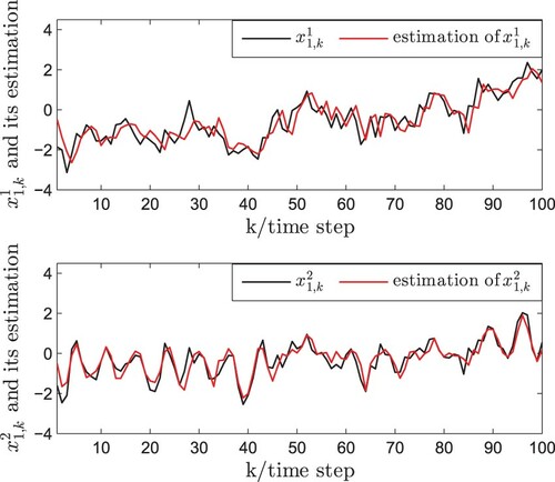
Figure 2. The trajectories of $x_{2,k}$ and its estimations.

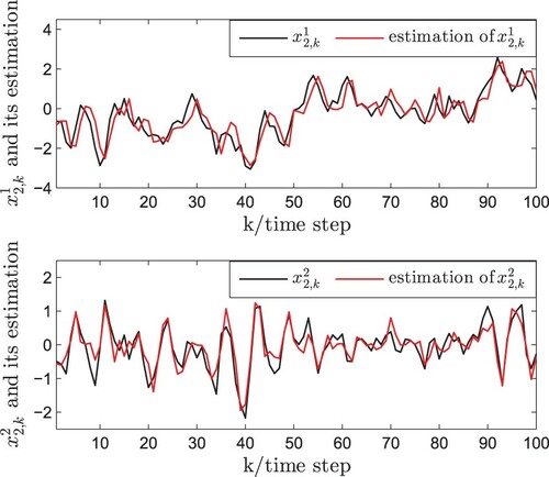
Figure 3. The trajectories of $x_{3,k}$ and its estimations.

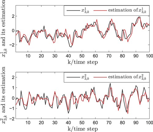
Figure 4. The trajectories of $x_{4,k}$ and its estimations.

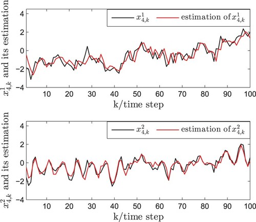
Figure 5. The trajectories of $x_{5,k}$ and its estimations.

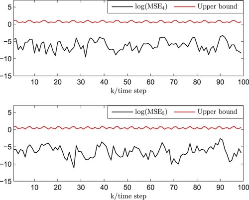
Let MSE${}_i(i=1,2,\dots ,5)$ be the mean square error (MSE) for the ith node. Figures 6 and 7 express the log (MSE) of the state $x_{i,k}$ and corresponding upper bounds $\log ({\mathrm{\Sigma }}_{i,k|k})$, which can verify that the MSE stays below the upper bounds. It can be seen that the proposed algorithm is effective.

Figure 6. log(MSE) with measurement outputs and corresponding upper bounds.

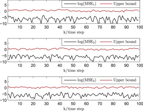
Figure 7. log(MSE) without measurement outputs and corresponding upper bounds.

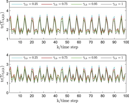
In order to further discuss the algorithm performance, the validity of new PNBSE method with the different probabilities of ROSD is illustrated by the simulations, which are plotted by Figures 8 and 9. The curves of tr(${\mathrm{\Sigma }}_{i,k|k}$) with measurement outputs are presented in Figure 8 under ${\overline{\gamma }}_{i,k}=0.25$, ${\overline{\gamma }}_{i,k}=0.75$, ${\overline{\gamma }}_{i,k}=0.95$, and ${\overline{\gamma }}_{i,k}=1$, the last two nodes without measurement outputs are shown in Figure 9. As can be seen from Figures 8 and 9, the nodes with measurement outputs and the nodes without measurement outputs can get the following conclusion: it can be observed the tr(${\mathrm{\Sigma }}_{i,k|k}$) is non-increasing when ${\overline{\gamma }}_{i,k}$ increase. This is the same conclusion as in Theorem 4.1. In conclusion, the above simulations show that the propose PNBSE algorithm is effective.

Figure 8. $\mathrm{tr}({\mathrm{\Sigma }}_{i,k|k})$ with measurement outputs under different probabilities (${\overline{\gamma }}_{i,k}$).

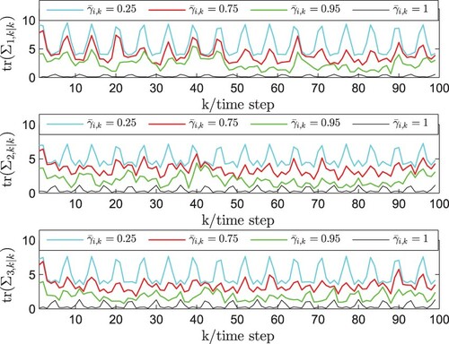
Figure 9. $\mathrm{tr}({\mathrm{\Sigma }}_{i,k|k})$ without measurement outputs under different probabilities (${\overline{\gamma }}_{i,k}$).

Remark 5.1

By means of variance-constraint method, the state estimation algorithms of complex networks have been given in W. Li et al. (2017a, 2017b), Hu, Wang, et al. (2020), and Hu et al. (2016) and the gain matrices of all nodes can be obtained. In this paper, the proposed PNB estimation algorithm is more appropriate for complex networks with a large number of nodes, which has the advantages in handling the case of the incomplete node's measurements. The simulation results show that PNB estimation algorithm can effectively estimate the states of entire complex networks, which could be seen from Figures 1–5. Moreover, the algorithm performance including the upper bound of estimation error covariance and the monotonicity analysis is discussed by the simulations. It can be seen from Figures 6–7 that the error of the proposed estimation method is bounded. Besides, it follows from Figures 8–9 that the theoretical result (i.e. monotonicity) obtained in Theorem 4.1 is rigorously demonstrated. Consequently, the performance of the estimator designed in this paper is good.

6. Conclusion

In this paper, a PNBSE algorithm has been proposed for linear complex networks with ROSD and SCS. The ROSD is expressed by a set of Bernoulli distributed random variables and the occurrence probabilities are assumed to be certain, and the SCS is represented by a set of random variables obeying the uniform distribution. By using the stochastic analysis method, a locally optimal upper bound has been obtained by constructing the estimator parameters, which was obtained by solving two Riccati-like difference equations. In addition, the theoretical analysis regarding the monotonicity of the estimation algorithm has been presented, i.e. it has been shown that estimation performance becomes worse if the ROSD is severe. Finally, some simulations have been provided to illustrate the validity and rationality of the new PNBSE method. The future research directions would be to extend the main research results to more complicated networks. Furthermore, we would discuss the applications of PNB estimation algorithm in different networked systems with network-induced phenomena such as neural networks, sensor networks, 2-D systems or other networks (Liang et al., 2018, 2019; L. Liu et al., 2020; Luo et al., 2017, 2020; Ma et al., 2020).

Disclosure statement

No potential conflict of interest was reported by the author(s).

Additional information

Funding

This work was supported in part by the National Natural Science Foundation of China [grant number 12071102].

References

- Baran, L., & Rzysko, W. (2020). Application of a coarse-grained model for the design of complex supramolecular networks. Molecular Systems Design & Engineering, 5(2), 484–492. https://doi.org/https://doi.org/10.1039/C9ME00122K
- Chen, D., Chen, W., Hu, J., & Liu, H. (2019). Variance-constrained filtering for discrete-time genetic regulatory networks with state delay and random measurement delay. International Journal of Systems Science, 50(2), 231–243. https://doi.org/https://doi.org/10.1080/00207721.2018.1542045
- Ding, R., Ujang, N., Bin Hamid, H., Abd Manan, M. S., Li, R., Albadareen, S. S. M., Nochian, A., & Wu, J. (2019). Application of complex networks theory in urban traffic network researches. Networks & Spatial Economics, 19(4), 1281–1317. https://doi.org/https://doi.org/10.1007/s11067-019-09466-5
- Gao, H., Dong, H., Wang, Z, & Han, F. (2020). An event-triggering approach to recursive filtering for complex networks with state saturations and random coupling strengths. IEEE Transactions on Neural Networks and Learning Systems, 31(10), 4279–4289. https://doi.org/https://doi.org/10.1109/TNNLS.5962385
- Hou, N., Wang, Z., Ho, D. W. C., & Dong, H. (2020). Robust partial-nodes-based state estimation for complex networks under deception attacks. IEEE Transactions on Cybernetics, 50(6), 2793–2802. https://doi.org/https://doi.org/10.1109/TCYB.6221036
- Hu, J., Cui, Y., Lv, C., Chen, D., & Zhang, H. (2020). Robust adaptive sliding mode control for discrete singular systems with randomly occurring mixed time-delays under uncertain occurrence probabilities. International Journal of Systems Science, 51(6), 987–1006. https://doi.org/https://doi.org/10.1080/00207721.2020.1746439
- Hu, J., Liu, G.-P., Zhang, H., & Liu, H. (2020). On state estimation for nonlinear dynamical networks with random sensor delays and coupling strength under event-based communication mechanism. Information Sciences, 511, 265–283. https://doi.org/https://doi.org/10.1016/j.ins.2019.09.050
- Hu, J., Wang, Z., & Liu, G.-P. (2020). Delay compensation-based state estimation for time-varying complex networks with incomplete observations and dynamical bias. IEEE Transactions on Cybernetics. https://doi.org/https://doi.org/10.1109/TCYB.2020.3043283
- Hu, J., Wang, Z., Liu, S., & Gao, H. (2016). A variance-constrained approach to recursive state estimation for time-varying complex networks with missing measurements. Automatica, 64, 155–162. https://doi.org/https://doi.org/10.1016/j.automatica.2015.11.008
- Hu, J., Wang, Z., Liu, G.-P., Jia, C., & Williams, J. (2020). Event-triggered recursive state estimation for dynamical networks under randomly switching topologies and multiple missing measurements. Automatica, 115, 1–13. https://doi.org/https://doi.org/10.1016/j.automatica.2020.108908
- Hu, J., Zhang, P., Kao, Y., Liu, H., & Chen, D. (2019). Sliding mode control for Markovian jump repeated scalar nonlinear systems with packet dropouts: The uncertain occurrence probabilities case. Applied Mathematics and Computation, 362, Article number: 124574. https://doi.org/https://doi.org/10.1016/j.amc.2019.124574
- Jia, C., Hu, J., Lv, C., & Shi, Y. (2020). Optimized state estimation for nonlinear dynamical networks subject to fading measurements and stochastic coupling strength: an event-triggered communication mechanism. Kybernetika, 56(1), 35–56. https://doi.org/https://doi.org/10.14736/kyb-2020-1-0035
- Kluge, S., Reif, K., & Brokate, M. (2010). Stochastic stability of the extended Kalman filter with intermittent observations. IEEE Transactions on Automatic Control, 55(2), 514–518. https://doi.org/https://doi.org/10.1109/TAC.2009.2037467
- Li, J., Dong, H., Wang, Z., & Bu, X. (2020). Partial-neurons-based passivity-guaranteed state estimation for neural networks with randomly occurring time delays. IEEE Transactions on Neural Networks and Learning Systems, 31(9), 3747–3753. https://doi.org/https://doi.org/10.1109/TNNLS.5962385
- Li, W., Jia, Y., & Du, J. (2017a). Non-augmented state estimation for nonlinear stochastic coupling networks. Automatica, 78, 119–122. https://doi.org/https://doi.org/10.1016/j.automatica.2016.12.033
- Li, W., Jia, Y., & Du, J. (2017b). Recursive state estimation for complex networks with random coupling strength. Neurocomputing, 219, 1–8. https://doi.org/https://doi.org/10.1016/j.neucom.2016.08.095
- Li, W., Jia, Y., & Du, J. (2017c). State estimation for on-off nonlinear stochastic coupling networks with time delay. Neurocomputing, 219, 68–75. https://doi.org/https://doi.org/10.1016/j.neucom.2016.09.012
- Li, W., Jia, Y., Du, J., & Fu, X. (2018). State estimation for nonlinearly coupled complex networks with application to multi-target tracking. Neurocomputing, 275, 1884–1892. https://doi.org/https://doi.org/10.1016/j.neucom.2017.10.012
- Liang, J., Wang, Z., & Liu, X. (2009). State estimation for coupled uncertain stochastic networks with missing measurements and time-varying delays: the discrete-time case. IEEE Transactions on Neural Networks, 20(5), 781–793. https://doi.org/https://doi.org/10.1109/TNN.2009.2013240
- Liang, J., Wang, F., Wang, Z., & Liu, X. (2018). Robust Kalman filtering for two-dimensional systems with multiplicative noises and measurement degradations: The finite-horizon case. Automatica, 96, 166–177. https://doi.org/https://doi.org/10.1016/j.automatica.2018.06.044
- Liang, J., Wang, F., Wang, Z., & Liu, X. (2019). Minimum-variance recursive filtering for two-dimensional systems with degraded measurements: Boundedness and monotonicy. IEEE Transactions on Automatic Control, 64(10), 4153–4166. https://doi.org/https://doi.org/10.1109/TAC.9
- Liu, D., Liu, Y., & Alsaadi, F. E. (2018). Recursive state estimation based-on the outputs of partial nodes for discrete-time stochastic complex networks with switched topology. Journal of the Franklin Institute, 355(11), 4686–4707. https://doi.org/https://doi.org/10.1016/j.jfranklin.2018.04.029
- Liu, L., Ma, L., Zhang, J, & Bo, Y. (2020). Sliding mode control for nonlinear Markovian jump systems with Denial-of-service attacks. IEEE/CAA Journal of Automatica Sinica, 7(6), 1638–1648. https://doi.org/https://doi.org/10.1109/JAS.6570654
- Liu, Y., Wang, Z., Ma, L., & Alsaadi, F. E. (2019). A partial-nodes-based information fusion approach to state estimation for discrete-time delayed stochastic complex networks. Information Fusion, 49, 240–248. https://doi.org/https://doi.org/10.1016/j.inffus.2018.12.011
- Liu, Y., Wang, Z., Yuan, Y., & Alsaadi, F. E. (2018). Partial-nodes-based state estimation for complex networks with unbounded distributed delays. IEEE Transactions on Neural Networks and Learning Systems, 29(8), 3906–3912. https://doi.org/https://doi.org/10.1109/TNNLS.2017.2740400
- Liu, Y., Wang, Z., Yuan, Y., & Liu, W. (2019). Event-triggered partial-nodes-based state estimation for delayed complex networks with bounded distributed delays. IEEE Transactions on Systems, Man, and Cybernetics: Systems, 49(6), 1088–1098. https://doi.org/https://doi.org/10.1109/TSMC.6221021
- Liu, S., Wei, G., Song, Y., & Liu, Y. (2016). Extended Kalman filtering for stochastic nonlinear systems with randomly occurring cyber attacks. Neurocomputing, 207, 708–716. https://doi.org/https://doi.org/10.1016/j.neucom.2016.05.060
- Luo, Y., Song, B., Liang, J., & Dobaie, A. M. (2017). Finite-time state estimation for jumping recurrent neural networks with deficient transition probabilities and linear fractional uncertainties. Neurocomputing, 260, 265–274. https://doi.org/https://doi.org/10.1016/j.neucom.2017.04.039
- Luo, Y., Wang, Z., Wei, G., & Alsaadi, F. E. (2020). Nonfragile l2- l∞ fault estimation for Markovian jump 2-D systems with specified power bounds. IEEE Transactions on Systems, Man, and Cybernetics: Systems, 50(5), 1964–1975. https://doi.org/https://doi.org/10.1109/TSMC.6221021
- Ma, L., Wang, Z., Hu, J., & Han, Q.-L. (2020). Probability-guaranteed envelope-constrained filtering for nonlinear systems subject to measurement outliers. IEEE Transactions on Automatic Control. https://doi.org/https://doi.org/10.1109/TAC.2020.3016767
- Shen, B., Wang, Z., Wang, D., & Li, Q. (2020). State-saturated recursive filter design for stochastic time-varying nonlinear complex networks under deception attacks. IEEE Transactions on Neural Networks and Learning Systems, 31(10), 3788–3800. https://doi.org/https://doi.org/10.1109/TNNLS.5962385
- Theodor, Y., & Shaked, U. (1996). Robust discrete-time minimum-variance filtering. IEEE Transactions on Signal Processing, 44(2), 181–189. https://doi.org/https://doi.org/10.1109/78.485915
- Wang, Z., Ho, D. W. C., & Liu, X. (2004). Robust filtering under randomly varying sensor delay with variance constraints. IEEE Transactions on Circuits and Systems II: Express Briefs, 51(6), 320–326. https://doi.org/https://doi.org/10.1109/TCSII.2004.829572
- Wang, L., Wang, Z., Huang, T., & Wei, G. (2016). An event-triggered approach to state estimation for a class of complex networks with mixed time delays and nonlinearities. IEEE Transactions on Cybernetics, 46(11), 2497–2508. https://doi.org/https://doi.org/10.1109/TCYB.2015.2478860
- Wen, C., Wang, Z., Liu, Q., & Alsaadi, F. E. (2018). Recursive distributed filtering for a class of state-saturated systems with fading measurements and quantization effects. IEEE Transactions on Systems, Man, and Cybernetics: Systems, 48(6), 930–941. https://doi.org/https://doi.org/10.1109/TSMC.2016.2629464
- Wu, Z.-G., Xu, Z., Shi, P., Chen, M. Z. Q., & Su, H. (2018). Nonfragile state estimation of quantized complex networks with switching topologies. IEEE Transactions on Neural Networks and Learning Systems, 29(10), 5111–5121. https://doi.org/https://doi.org/10.1109/TNNLS.2018.2790982
- Zhang, H., Hu, J., Liu, H., Yu, X., & Liu, F. (2019). Recursive state estimation for time-varying complex networks subject to missing measurements and stochastic inner coupling under random access protocol. Neurocomputing, 346, 48–57. https://doi.org/https://doi.org/10.1016/j.neucom.2018.07.086
- Zou, L., Wang, Z., Hu, J., & Zhou, D. (2020). Moving horizon estimation with unknown inputs under dynamic quantization effects. IEEE Transactions on Automatic Control, 65(12), 5368–5375. https://doi.org/https://doi.org/10.1109/TAC.9
- Zou, L., Wen, T., Wang, Z., Chen, L., & Roberts, C. (2019). State estimation for communication-based train control systems with CSMA protocol. IEEE Transactions on Intelligent Transportation Systems, 20(3), 843–854. https://doi.org/https://doi.org/10.1109/TITS.2018.2835655