Fault detection and diagnosis of linear bearing in auto core adhesion mounting machines based on condition monitoring

Abstract

This study aims to increase machine reliability thereby preventing product defects from adhesive dispense and slider attachment by a fault detection and diagnostic technique. The experiment was set up to investigate the vibration signal and motor current. Six fault conditions of a linear bearing were set up. The approaches, including spectrum analysis, crest factor, and analysis of variance, are used for data analysis. It was found that the spectrum analysis was suitable for classifying the frequency domains and the statistics tool was successful in measuring the current. Fault detection and diagnosis results can forecast the status of the linear bearings.

KEYWORDS:

• Fault detection and diagnosis
• linear bearing
• analysis of variance
• spectrum analysis
• crest factor
• motor current

1. Introduction

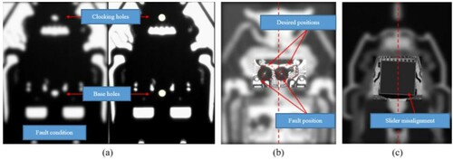
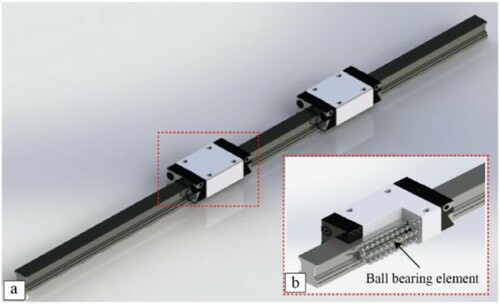
The head gimbal assembly (HGA), shown in Figure 1, is the major component used in hard disc drive for reading and writing the data. The HGA consists of two main components: the slider (magnetic recording head) and the suspension (Deeying et al., 2018). The HGA assembly process includes adhesive dispensing, slider attachment, adhesive curing, and soldering, as shown in Figure 2(a–d). The first stage in the HGA assembly process is to attach the slider to the suspension following product specifications. The slider attachment process is achieved by the use of the auto core adhesion mounter (ACAM) machine, as shown in Figure 3(a), which is used for adhesive dispensing and attaching the slider onto the suspension. This requires sub-micron accuracy in the positioning of the slider. The machine proceeds by clamping the suspension to the desired position, then the identified two datum holes, located on the base and the clocking hole on the suspension, are utilized for reference data to process the adhesive dispense and slider attachment location on the suspension. In order to move the suspension into the desired position, the clamping unit is driven by a linear DC motor that is linked to the linear bearings, as shown in Figure 3(b). The machine runs continuously at a high speed in order to comply with the manufacturer’s requirements. Deterioration of moving parts is unavoidable. The linear bearings are the most susceptible parts which tend to deteriorate quickly and become contaminated due to the openness of the structure. Degeneration of the linear bearing causes the machine to vibrate as a result of which the reference holes become blurred etc., as shown in Figure 4(a). These faults directly impact machine performance, thereby reducing the capability of the adhesive dispenser and slider attachment accuracy and reliability, as shown in Figure 4(b,c). Therefore, fault detection and diagnosis of the linear bearings is very important to foster prevention rather than detection of dispensing and slider attachment positioning errors.

Figure 1. Head gimbal assembly (HGA).

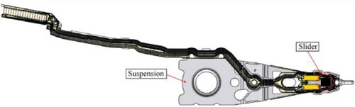
Figure 2. HGA process (a) Adhesive dispensing, (b) Slider attachment, (c) Adhesive cure and (d) Soldering.

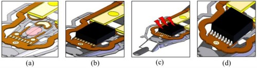
Figure 3. (a) ACAM machine and (b) clamping unit in ACAM machine.

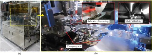
Figure 4. (a) The impact of vibrations on reference hole positioning and (b) fault position of adhesive dispensing and (c) attached slider misalignment.

The reviews on the related fault detection will be provided as follows. The fault detection is an approach in linear bearings of brushless AC linear motors, using a signal processing technique that analyses the vibration signals. It was found that the characteristic frequency of faults was detected most effectively was a suitable technique (Bianchini et al., 2011). This work was proposed using both cyclostationary and kurtosis spectrum analyses for the frequency selection for detecting improperly lubricated bearing, in which the most varied vibration patterns are expressed. The methods evaluated in the test kit consist of 63 fault-free electric motors and 21 improperly lubricated bearings. The results showed that improper lubrication was caused by an increase in the spectrum component at the bearing cage and the rotation frequency of the ball (Boškoski et al., 2010). The analytical approximate response of the nonlinear system for the milling process is estimated through multiple approaches by testing under the steady-state condition. The effects of structural nonlinearity, cutting force coefficients and tool wear length, and process damping were investigated by the frequency response functions. Finally, the comparison of primary and supper harmonic resonance shows low spindle speed is preferable to keep low vibration amplitude (Moradi et al., 2013). The Condition Monitoring and Fault Diagnostics (CMFD) system for hydropower plants with Support Vector Machine (SVM) for fault diagnostics was conducted. The analysis of SVM in the Virtual Diagnostic Center (VDC) allows all stakeholders accessible from anywhere and anytime, the service provider can establish condition-based maintenance and offer operation support for better maintenance (Selak et al., 2014). A rapid cartogram algorithm can be used to obtain optimal centre frequency and bandwidth of the band-pass filter base with maximum spectrum kurtosis. As a result, there was a discussion of how to eliminate the frequency – smear problems (in the spectrum) and of the fault diagnostics of the rolling element bearing in the variable-speed running conditions of rotating machinery achieved by using learning techniques (Guo et al., 2012). The broken rotor bar of an induction motor was detected and located. The Hilbert Transform was introduced for the analysis of a start-up stator current envelope based on statistics. The result obtained is possible to diagnose and detect the exact location of the rotor fault (Abd-el-Malek et al., 2017). The main differences between the conventional neural networks was a deep learning method which provides for image recognition to be used for intelligent fault diagnosis of rolling bearing bases to establish a healthy-state classification and a comparison experiment was conducted to test whether efficiency greater than 90% was achieved with fewer computational resources for the use of learning techniques (Lu et al. 2017). The challenges in the Kalman filter are used to estimate the pitch rate from the elevator deflections and used for adapting the control power elevator according to current flight conditions. This method was used to test small fixed wings, by utilizing the input-output ratio for fault detection and identification (Weimer et al., 2012). Using the diagnostic method, a hazard and operability study (HAZOP) module is incorporated into a fault diagnosis. Based on Petri Nets that entitled the case study of a hydropower plant, the information obtained in the risk analysis is very useful for the development of a goal-oriented model, which, in turn, can be used to assist the automatic fault diagnosis. Melani et al., 2016 have recently developed monitoring, diagnostic, prognostic and health management (PHM) technologies to improve and enhance maintenance control strategies for manufacturing operations to improve asset availability, product quality and overall productivity. The optical interferometer was applied for measuring the force acting on the moving parts of pneumatic linear bearings. The results show the capability of detecting the fault of friction force (Nakamura et al., 2004). The paper on a novel model of one-class bearing fault detection, using a real-valued negative clone selection algorithm (RNCS) based on higher order statistics (HOS), discusses how the algorithm can detect faults in bearings by using real-valued negative clone selection. The results show the effectiveness of classifiers in the detection of bearing condition (Xin-min et al., 2007). This research established a method to diagnose faults in bearings based on Empirical Mode Decomposition (EMD) and an envelope spectrum. The method was applied to a machine tool with ball bearings. It was found that EMD and an envelope spectrum could detect anomalies in bearings (Zhang & Ai, 2008). In addition, the diagnosis could also be used for the detection of the stator current, damage to bearings and a comparison of the two conditions in an experiment. However, the results revealed that the health of the bearings depends on the amount of the load. Mbo'o & Hameyer, 2015 reported that the Hilbert-Huang transform can be utilized to determine the optimal condition if the degeneration features are extracted. The proposed method predicts the remaining useful life (RUL) of bearings accurately (Liu et al., 2018). The kurtosis and spectrum analysis was applied in the detection of generalized roughness and single-point bearing faults using a linear prediction-based current noise cancellation and the results of the experiment confirm that the condition of the bearings can be classified (Dalvand et al., 2018). The new approach Spindle Condition Estimate device (SCED) was developed to collect data and segregate the system dynamics from defect. The approach was shown capable of detecting a defect-driven diagnostic method for machine tool spindles (Vogl & Donmez, 2015). The Initial Measurement Unit (IMU) was developed for diagnosing the machine condition to minimise interrupt to production. The data from IMU used to identify the changes in translation and angular error of degradation and observe the performance of machine tool. It was found that the IMU-based method was capable of measuring the geometric errors with acceptable test uncertainty ratios (Vogl et al., 2016). A dynamic analysis was reported in terms of mechanical actions and mechanical vibrations to develop a monitoring and diagnostic approach to a three-dimensional case and the synchronous envelope analysis (SEA) was used in the monitoring process. SEA is an appropriate dynamic predictive technique at high frequencies (Bisu et al., 2013). The article presented a non-contact excitation method for evaluating the dynamic stiffness of a rotating spindle and for predicting the chatter condition and monitor oscillations under regenerative force feedback. It was found that the speed effect was influenced by the spindle temperature (Matsubara et al., 2015). A new condition indicator (CI) has proposed Amplitude of Probability Density Function (APDF) for the residual vibration detection. The effect of combined noise and vibration can be predicted using the discomfort model derived. The data used contain a full history of the progressively deteriorating gear condition – from a healthy condition until a catastrophic failure. The concept of the proposed new CI and its results has been compared to the FM4 method indicator (Rzeszucinski et al., 2012). The article conducted the experiment by signal processing and Artificial Neural Network (ANN) with feed-forward approaches to detect the multiple fault conditions of the induction motors. The Continuous Wavelet Transform (CWT) was used for feature extraction from the stator current signals. The result was shown successfully with 100% accuracy (Jawadekar et al., 2014). The fault diagnosis of the bearing by the vibration signal can be applied to the convolutional neural network, which has a high ability for feature extractor and classifies the data, which is an end-to-end diagnosis method (Li et al., 2019). However, there are fewer supporting documents for fault detection and diagnostics in linear bearing applications in high speed automation machines.

This research aims to increase ACAM machine reliability and prevent defects from adhesive dispensing and slider attachment processes by using fault detection and diagnostic techniques. The experiment investigates the use of vibration signals and motor current for fault detection and diagnostics. Six conditions of linear bearings, including healthy, starved lubrication, ball bearing damage, ball bearing damage with starved lubrication, ball bearing loss and ball bearings loss with starved lubricants, were set up. Three approaches were used for the data analysis, which included spectrum analysis, the crest factor and analysis of variance (ANOVA).

2. Linear bearings model for vibration analysis

Linear bearings in Figure 5(a) are mainly designed to support the linear motions of a machine, reduce its friction and facilitate the fluent motion of a linear axis. The linear bearing component consists of a carriage and a rolling element. In the operation, the ball bearing elements (Figure 5(b)) recirculate within a runner block and move together along the linear guide rail in order to maintain a smooth motion for the machine. Linear bearings are used on machines that run at high speed of motion when in operation. However, it is an open structure that is prone to collecting contamination resulting in the main factor causing failure of the linear bearing. The phenomenon that we detect before the linear bearing failure is known as the fault condition. This condition can generate a vibration signal which is different from that of a healthy condition. The vibration signal, when a linear bearing fault is detected, is a combination of each component. This is the main reason for defining the parameters of the linear bearings for vibration analysis.

Figure 5. (a) Linear bearing and (b) ball bearing element.

The physical parameters of the linear bearings, shown in Figure 6, are important in addressing fault frequency and analytical phenomena of the vibration signals when the parameters of the linear bearings change.

Figure 6. Ball bearing structure and physical parameters.

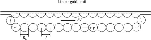
In Figure 6, $Db$ is the diameter of the ball bearing element, $l$ is the pitch of the ball bearing and speed of the linear motor is defined by $v$.

2.1. Ball bearing damaged

The effect of the ball bearing damage on recirculation occurs when the defective area hits the rail which produces a fault each time. The characteristic frequency of the fault is defined in Equation (1). When $f_{\text{ball}}$ defines as ball element fault characteristic frequency. $Db$ is the ball diameter and v is the speed of the linear motor. The amplitude of the vibration will occur when the damaged ball bearing is under load which means the ball is acting between the rail and the carriage; however, if the damaged ball bearing is not under load, the vibration will not occur. Additionally, the motor speed also affects the frequency of faults, as shown in Table 1. The spectrum of the vibration signal of both healthy and fault condition is shown in Figure 7(a,b). (1) $f_{\text{ball}}=\frac{2v}{\pi D_b}$(1)

Figure 7. Spectrum of the vibration signal.

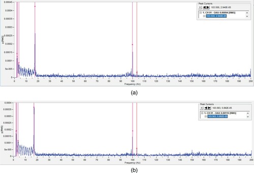
Table 1. The influence of speed on fault frequency.

Motor speed (m/s)	Ball speed (m/s)	Fault frequency (Hz)
0.25	0.125	26.5
0.50	0.200	53.0
1.00	0.500	106.0

2.2. Ball bearing loss

The performance of the ball bearing recirculation is an important factor in the linear bearing movement. As the fault frequency of the rail or carriage, the expected frequency response is shown in Equation (2). It depends on two factors: the speed of a motor ($v$) and the pitch distance of ball bearing element ($l$). When the ball bearing loss causes the change in the fault frequency, the pitch distance of ball bearing increases. (2) $f_{\text{rail}}=f_{\text{carriage}}=\frac{v}{l}$(2)

2.3. Starved lubricant bearing

The lubricant is a critical part of the linear bearing operation because it provided separation between ball bearing and cage reducing wear. The lubricant also prevents corrosion of the ball bearing element; however, after the prolonged operation, the linear bearing may become starved of lubricant. This problem affects the operation of linear bearing in high friction conditions, which causes the component to rapidly wear. To detect such a condition, an investigation into the vibration amplitude was conducted. In the case of improper lubrication, the contact between the ball elements, rail and carriage will excite fluctuations in the amplitudes and periods of occurrence of the impulse response, as shown in Equation (3). (3) $x(t)=\sum _{i=-\mathrm{\infty }}^{+\mathrm{\infty }}{A}_{i}s(t-iT-{\tau }_i)+n(t)$(3) where $A_i$ is the random amplitude and iT is the impulse response, ${\tau }_i$ is the time fluctuation between two infectious impulse responses and $n(t)$ defines an additive random component that contains all non-modelled vibrations as well as environmental disturbances.

3. Fault detection and diagnosis

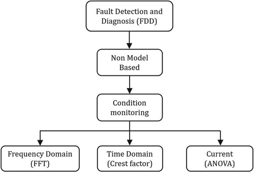
In order to prevent faults in a machine, it is vital to protect the machine and perform regularly scheduled maintenance. Fault detection and diagnosis (FDD) is one of the approaches to detect and diagnose the failure. When the component failure happens prior to the scheduled maintenance, the FDD system alerts or alarms technician or engineer to involve or select the appropriate controller to reconfigure the system to maintain the system to run with the desired condition. Therefore, FDD is used to detect the deterioration of a component to prevent rather than detect a machine performance issue. The FDD can distinguish two techniques: model based and non-model based. This work uses the vibration signals with frequency domain, time domain and the current of the motor. he fault condition of the linear bearing is shown in Figure 8 for analysis.

Figure 8. FDD non-model-based classification.

4. Signal processing technique

4.1. Frequency-domain analysis

In most cases, the presence of damage will cause an effect related to the movement of the system. Then, if the movement system is periodic, the impact will also be periodic. The frequency of effects can be detected in the spectrum (Bianchini et al., 2011). Analysis in the frequency domain is the most important technique used. The signal spectrum is calculated by Fourier decomposition, which is defined in Equation (4) (4) $X(f)=\frac{1}{T}{\int }_{-\frac{T}{2}}^{\frac{T}{2}}x(t).e^{-i2\pi ft}dt$(4) Usually, the presence of a fault on a moving element modulates the amplitude of the vibration signal with a frequency which is characteristic of the damage.

The difference in the amplitude of spectrum to small is difficult to distinguish; therefore, the analysis of amplitude in $dB$ unit was useful. The equation is given as follows: (5) $f(x)=20{\log }_{10}[X(t)]$(5)

4.2. Crest factor

The crest factor is defined as the ratio between the maximum peak values divided by the root mean square (RMS) of the signal, shown as follows: (6) $C=\frac{|x{(t)}_{\text{peak}}|}{x{(t)}_{\text{rms}}}$(6) This indicator states the significance of impulsive phenomena such as those correlated with an impact between the bearing elements with respect to the RMS value of the signal. The results indicate a small peak value in the case of a normal condition; however, a large peak value indicates faulty conditions as the crest factor is large.

4.3. Analysis of variance

Analysis of variance (ANOVA) can be specified in terms of statistical techniques and mathematical models that are useful for testing the comparability of several means of response which are affected by the number of input variables used to optimise the means..Thus, the experimental design is a completely randomised design, which can be formulated by Equation (7). (7) $y_{ij\sim }N(\mu +{\tau }_i,{\sigma }^2)$(7) where $y_{ij}$ is the response $ij\text{th}$ observation; $N$ is the observation sample number; $\mu$ is the constant and the treatment effects; ${\tau }_i$ is the parameter unique to the $i\text{th}$ treatment effect; ${\sigma }^2$ is the variance assumed to be constant for all levels of the factor which implies that the observations are mutually independent.

In the analysis of estimation for the parameter, the definition is implied in the following equation: (8) $\sum _{i=1}^a{\tau }_i=0$(8) That is the treatment or factor effects employed thought of deviation from the overall mean. The different levels of confidence in comparing multiple factors used the Fisher least significant difference (LSD) method to find a simultaneous confident level from the individual error rate. This method uses the t-statistic to indicate a comparison of all the pairs of means. To observe the factor-level differences between the populations mean, the equation for t-statistic value to the t-distribution to determine mean difference can be expressed by Equation (9). (9) $t_0=\frac{{\overline{y}}_{i.}-{\overline{y}}_{j.}}{\sqrt{\text{M}{\text{S}}_E((1/n_i)+(1/n_j))}}$(9) where $t_0$ is the statics for testing hypothesis assumption. $\text{M}{\text{S}}_E$ is the mean squared deviation thought measurement the average square of the error. $n_i,n_j$ is the sample size independent variables.

5. Experiment and results

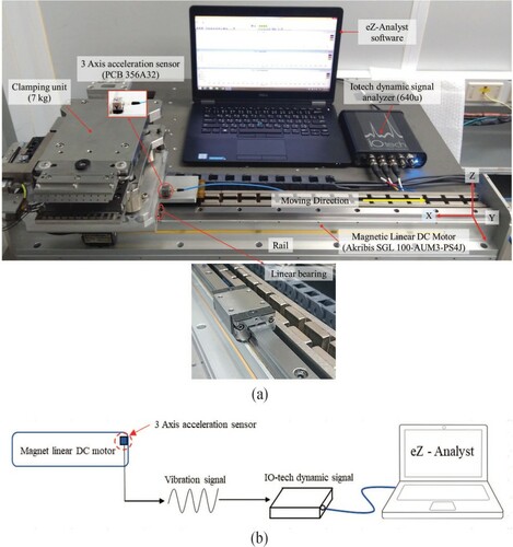
To set up the experiment same conditions as machine in manufacturing, a magnet linear dc motor akribis SGL 100-AUM3-PS4J was used. The clamping unit was installed to demonstrate the load condition with the weight of 7 kg on the top worktable of the magnet linear dc motor, as shown in Figure 9(a). The data acquisition, the linear motor movement, was controlled in one direction and the vibration signal was captured by the IO-tech dynamics signal analyser PCB Piezotronics model 356A32 which was used by installing a three-axis acceleration sensor at a nominal sensitivity of 99.2 mV/g for x-axis, 98.1 mV/g for y-axis and 101.1 mV/g for z-axis. The sensor was placed on the top of the linear bearing with the x-axis parallel to the direction of the linear movement and relative to the z-axis perpendicular to the floor plane, as shown in Figure 9(b). A frequency signal was acquired via the ez – analyser program with a sampling frequency of 4000 Hz. In order to record the current of the linear motor, the akribis PC Suite program was used. The experiment was conducted with motor speed varying by 0.25, 0.5, and 1 m/s to simulate the machine run, as manufacturing requirement.

Figure 9. (a) The experiment set-up and (b) DAQ system.

The experiment was conducted by using five faulty conditions of the linear ball bearings to compare with a healthy condition. The fault conditions were set up by three conditions which are single-fault condition including all bearing damaged, ball bearing loss and the starved lubricant bearing. The simulation of each condition is shown as follows:

5.1. Ball bearing damaged

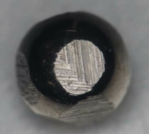
One ball bearing damaged was simulated by manual grinding the surface of the ball bearing, as shown in Figure 10. The area of damage was 1.327 mm².

Figure 10. Microphotograph of the damage on the ball bearing element.

5.2. Ball bearing loss

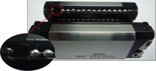
The simulation of the ball bearing loss is to demonstrate the fault condition of linear bearing. When the ball bearing loss cause the pitch distance of ball bearing will change and cause the frequency of the linear ball bearing will different from the health condition.

The set-up of the ball bearing loss is shown in Figure 11.

Figure 11. Ball bearing loss.

5.3. Starved lubricant bearing

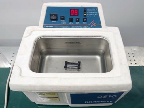
The lubricant is used for friction reduction and corrosion protection is proposed. The experiment was set up to remove lubricant from linear ball bearing by using isopropyl alcohol cleaner with BRANSON (2510 model) digital ultrasonic cleaning machine, as shown in Figure 12.

Figure 12. Removal of contaminate and lubricant using ultrasonic cleaner.

5.4. Combination of fault conditions

In general, the phenomena of faults in linear bearings can occur to more than one component that is damaged; therefore, a combination of faults was also investigated. Based on a combination of faulty conditions, the simulation of ball bearing damage with starved lubricant and ball bearing loss of lubricant was validated. However, the fault frequency of these conditions will be different for a single fault and a healthy condition.

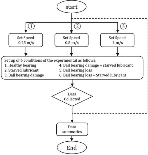
A sequence of experiments was conducted, as in Figure 13, from which the data of vibration in both the time and frequency domain were obtained as well as the motor current value for each condition so that the sample size was equal to 50 data samples. Besides, the speed of the linear motor was adjusted and varied between 0.25, 0.5, and 1 m/s based on real production requirements.

Figure 13. The sequence of data collected.

5.5. Spectral analysis

A spectral analysis was conducted for fault detection in healthy and faulty linear bearings. According to spectral signal and box plot of the spectrum shown in Figures 14–16, a comparison of the spectrum from the experimental data along the x-axis for the six conditions was carried out with varying motor speeds at 0.25 m/s (26.5 Hz), 0.5 m/s (53 Hz) and 1 m/s (106 Hz).

Figure 14. (a) Spectrum signal; (b) box plot of spectrum signal at speed 0.25 m/s $(f_{\text{ball}}=26.5\text{Hz})$.

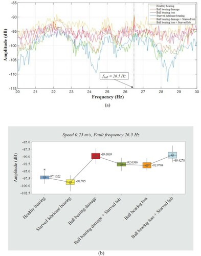
Figure 15. (a) Spectrum signal; (b) box plot of spectrum signal at speed 0.50 m/s $(f_{\text{ball}}=53\text{Hz})$.

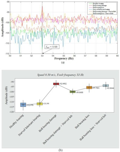
Figure 16. (a) Spectrum signal; (b) box plot of spectrum signal at speed 1.0 m/s $(f_{\text{ball}}=106\text{Hz})$.

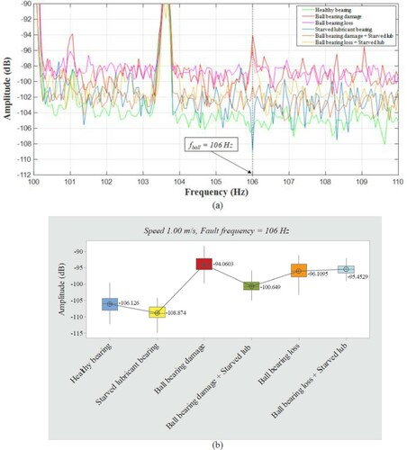
All three motor speeds and the spectrum signal showed the amplitude of a ball bearing damaged, ball bearing loss, ball bearing damaged with starved lubricant and a ball bearing loss with starved lubricant showed higher amplitude signal compared with healthy and starved lubricant conditions. The box plot distinguishes two groups of data. The first group is healthy and starved lubricant conditions with lower amplitude compared with the other four conditions. This indicates that the spectral analysis can distinguish the four fault conditions of the linear bearing from the healthy condition; however, starved lubricated is not different compared with the healthy bearing. All three motor speeds showed a similar trend of spectrum signal data.

5.6. Motor current analysis

The motor current data were collected 50 data sets for each bearing condition; the analysis was conducted by the ANOVA method used to determine the variable currents which are applied to healthy and faulty bearing conditions. Minitab 17 software was used to establish mathematical models and to identify the analysis revealed by the ANOVA response function. The results of the ANOVA analysis for the motor current responses of all three motor speeds are shown in Tables 2–4 (F-values and P-values of each term are provided).

Table 2. Analysis of variance of current at a motor speed of 0.25 m/s.

Analysis of variance
Source	DF	Adj SS	Adj MS	F-value	P-value
Factor	5	215,314	43,062.8	498.57	0.000
Error	294	25,393	86.4
Total	299	240,707
Model summary
S	R-sq	R-sq (adj)	R-sq (pred)
9.29367	89.45%	89.27%	89.02%
Fisher pairwise comparisons
Grouping information using the Fisher LSD method and 95% confidence
Factor	N	Mean	Grouping
Ball bearing loss + Starved lub	50	1029.88	A
Ball bearing damage + Starved lub	50	933.4	B
Ball bearing damage	50	983.44	C
Ball bearing loss	50	965.32	D
Starved lubricant bearing	50	958.46	E
Healthy bearing	50	949.22	F

Note: Means that do not share a letter are significantly different.

Table 3. Analysis of variance of current at a motor speed of 0.50 m/s.

Analysis of variance
Source	DF	Adj SS	Adj MS	F-value	P-value
Factor	5	1,618,742	3237.48	707.04	0.000
Error	294	134,621	458
Total	299	1,753,363
Model summary
S	R-sq	R-sq(adj)	R-sq(pred)
21.3985	92.32%	92.19%	92.01%
Fisher pairwise comparisons
Grouping information using the Fisher LSD method and 95% confidence
Factor	N	Mean	Grouping
Ball bearing loss + Starved lub	50	1286.08	A
Ball bearing damage + Starved lub	50	1144.78	B
Ball bearing damage	50	1104.48	C
Ball bearing loss	50	1097.90	CD
Starved lubricant bearing	50	1093.93	D
Healthy bearing	50	1060.56	E

Note: Means that do not share a letter are significantly different.

Table 4. Analysis of variance of current at a motor speed of 1.00 m/s.

Analysis of variance
Source	DF	Adj SS	Adj MS	F-value	P-value
Factor	5	1,354,029	270,806	562.88	0.000
Error	294	141,447	481
Total	299	1,495,476
Model summary
S	R-sq	R-sq (adj)	R-sq (pred)
21.9342	90.54%	90.38%	90.15%
Fisher pairwise comparisons
Grouping information using the Fisher LSD method and 95% confidence
Factor	N	Mean	Grouping
Ball bearing loss + Starved lub	50	1322.28	A
Ball bearing damage + Starved lub	50	1281.96	B
Ball bearing damage	50	1188.98	C
Ball bearing loss	50	1183.44	C
Starved lubricant bearing	50	1170.30	D
Healthy bearing	50	1128.68	E

Note: Means that do not share a letter are significantly different.

5.6.1. Analysis of variance of current at motor speed 0.25 m/s

The ANOVA analysis for the current voltage is given in Table 2. It can be observed that if the p-value is lower than 0.05, there is a significant effect to determine individual factor means are different variables to experiment response and the probability is over 95%. The coefficient of determination $R^2$ = 89.45%, adjusted $R^2$ = 89.27%, predicted $R^2$ = 89.02% in such a way that whenever these three values are close to each other they tend to be 100%. The observation values indicate compared confidence interval pairs of means observed conditions are significantly different for all bearing conditions. The motor current of all six bearing condition is different, as shown in Table 2. The highest motor current is the ball bearing loss with starved lubricant and the lowest of motor current is the healthy bearing condition. At speed 0.25 m/s the motor current can be classified for the bearing condition.

5.6.2. Analysis of variance of current at motor speed 0.50 m/s

The ANOVA results for the motor speed of 0.5 m/s in the model are shown in Table 3. The p-value is less than .05 and the adequacy of the model is $R^2$ = 92.32%, adjusted $R^2$ = 92.19%, and predicted $R^2$ = 92.01%, respectively, which confirms the experiment model. Based on the LSD comparison method, a healthy bearing is significantly different from other faults. However, the ball bearing damage, ball bearing loss, and starved lubricant bearing showed comparable because the motor current value shows slightly different.

5.6.3. Analysis of variance of current at motor speed 1.0 m/s

The ANOVA table of the regression model is given in Table 4. The associated p-value of less than .05 indicates that the terms of the model are statistically significant. The other adequacy measures are: $R^2$ = 90.54%, adjusted $R^2$ = 90.38%, and predicted $R^2$ = 90.15% are in reasonable agreement and are close to 1. A healthy bearing result shows a significant different in motor current relative to other conditions. This indicates that ball bearing loss and ball bearing damage show no significant difference with the motor current value 1183.44 and 1188.98 mA, respectively.

The summary of motor current is shown in Table 5. The motor current is suitable for bearing condition classification. The healthy condition showed different value of motor current compared with other conditions for all three motor speeds. The starved lubricant can segregate from the healthy bearing condition for all speeds. The combination of fault condition showed a significant difference from other conditions. The influence of motor speed increasing shows an increase of the motor current for each bearing condition is helpful for bearing condition classification.

Table 5. Summary of motor current for all bearing conditions.

	Current (mA)			% Increase of motor current
Bearing condition	0.25 m/s	0.5 m/s	1.0 m/s	0.25 m/s	0.5 m/s	1.0 m/s
Ball bearing loss + starved lubricant	1029.88	1286.08	1322.28	8.50%	21.26%	17.15%
Ball bearing damage + starved lubricant	993.40	1144.78	1281.96	4.65%	7.94%	13.58%
Ball bearing damage	983.44	1104.48	1188.98	3.61%	4.14%	5.34%
Ball bearing loss	965.32	1097.90	1183.44	1.70%	3.52%	4.85%
Starved lubricant bearing	958.46	1093.92	1170.30	0.97%	3.15%	3.69%
Healthy bearing	949.22	1060.56	1128.68	0.00%	0.00%	0.00%

5.6.4. Crest factor analysis

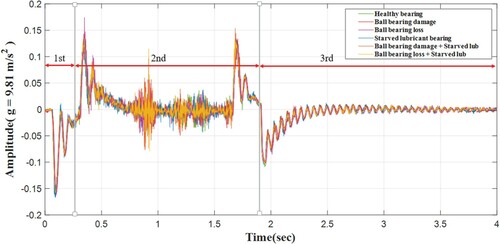
The results of the vibration signals validated in the time domain showed the response for all six conditions of three motor speeds, shown in Figure 17. The vibration response represents the signal followed by the influence of beginning of the motor which showed high acceleration, the second one showed the vibration response, while the linear bearing is moving along the linear guide rail and the last is the response of deceleration. To classify bearing condition, the crest factor is proposed to use.

Figure 17. Vibration signals in the time domain.

A comparison summarises the crest factor value of the linear bearing for all three motor speeds. The result of crest factor comparison for all three motor speed showed the value of each condition is slightly different from healthy bearing which can be concluded that the crest factor is not suitable for use to classify linear bearing condition, as shown in Tables 6–8.

Table 6. Crest factor comparison of faulty conditions (0.25 m/s).

Target	Bearing condition	Avg	Delta	%
Healthy	Ball bearing loss + starved lubricant	3.98	0.30	8
	Ball bearing damage + starved lubricant	3.97	0.29	8
	Ball bearing damage	4.07	0.39	11
	Ball bearing loss	4.14	0.46	12
	Starved lubricant bearing	3.79	0.10	3

Table 7. Crest factor comparison of faulty conditions (0.5 m/s).

Target	Bearing condition	Avg	Delta	%
Healthy	Ball bearing loss + starved lubricant	4.05	0.25	7
	Ball bearing damage + starved lubricant	4.17	0.37	10
	Ball bearing damage	4.19	0.39	10
	Ball bearing loss	4.20	0.40	11
	Starved lubricant bearing	4.05	0.25	7

Table 8. Crest factor comparison of faulty conditions (1.0 m/s).

Target	Bearing condition	Avg	Delta	%
Healthy	Ball bearing loss + starved lubricant	5.65	0.28	5
	Ball bearing damage + starved lubricant	5.66	0.29	5
	Ball bearing damage	5.80	0.43	8
	Ball bearing loss	5.78	0.41	8
	Starved lubricant bearing	4.86	0.49	9

6. Conclusion

This paper investigated fault detection and diagnostic techniques used for increasing ACAM machine reliability for preventing defects of adhesive dispensing and slider attaching processes. Experimental design and hypothesis testing are considered based on actual manufacturing process. Thus, fault detection and diagnosis of linear bearings are studied by applying three approaches: spectrum analysis, the crest factor, and ANOVA with three-speed variations required for production rates. The six conditions included with single and combination fault of a linear bearing were tested and analysed. The key results are summarised as follows:

1. The result shows motor current with ANOVA test is suitable to classify the condition of a linear bearing single and combination relative to the healthy condition.

2. The influence of motor speed increase shows that different motor current for each bearing condition is helpful for bearing condition classification.

3. The spectrum signal analysis was able to distinguish healthy from fault condition. However, the starved lubricant condition showed comparable relative to the healthy condition.

4. The crest factor is not an appropriate technique for the classification of linear bearing condition. Although the speed increase shows possible detection, the differences are small and not suitable for use without further optimisation and investigation.

5. The effectiveness of each parameter is not equal for fault detection and diagnosis of linear bearing conditions. In the future, the status of the automation machine will be decided by machine learning which needs more parameters and data.

6. Furthermore, the spectrum analysis, crest factor and analysis of variance techniques are combined to investigate the performance for detection and diagnostic of the bearing condition.

7. The result reveals the fault detection by the motor current is the suitable technique that can be applied to classify the linear bearing condition for the auto core adhesion mounting machines to improve the reliability and preventing defects.

Disclosure statement

No potential conflict of interest was reported by the author(s).

Additional information

Funding

This research was supported by the Research and Researcher for Industry (RRI) under the Thailand Research Fund (TRF). It offers a scholarship for PhD students at Suranaree University of Technology (SUT) through [grant number PHD60I0043].

References

- Abd-el-Malek, M., Abdelsalam, A. K., & Hassan, O. E. (2017). Induction motor broken rotor bar fault location detection through envelope analysis of start-up current using Hilbert transform. Mechanical Systems and Signal Processing, 93, 332–350. https://doi.org/https://doi.org/10.1016/j.ymssp.2017.02.014
- Bianchini, C., Immovilli, F., Cocconcelli, M., Rubini, R., & Bellini, A. (2011). Fault detection of linear bearings in brushless AC linear motors by vibration analysis. IEEE Transactions on Industrial Electronics, 58(5), 1684–1694. https://doi.org/https://doi.org/10.1109/TIE.2010.2098354
- Bisu, C., Olteanu, L., Laheurte, R., Darnis, P., & Cahuc, O. (2013). Experimental approach on torsor dynamic analysis for milling process monitoring and diagnosis. Procedia CIRP, 12, 73–78. https://doi.org/https://doi.org/10.1016/j.procir.2013.09.014
- Boškoski, P., Petrovčič, J., Musizza, B., & Juričić, Đ. (2010). Detection of lubrication starved bearings in electrical motors by means of vibration analysis. Tribology International, 43(9), 1683–1692. https://doi.org/https://doi.org/10.1016/j.triboint.2010.03.018
- Dalvand, F., Kang, M., Dalvand, S., & Pecht, M. (2018). Detection of generalized-roughness and single-point bearing faults using linear prediction-based current noise cancellation. IEEE Transactions on Industrial Electronics, 65(12), 9728–9738. https://doi.org/https://doi.org/10.1109/TIE.2018.2821645
- Deeying, J., Asawarungsaengkul, K., & Chutima, P. (2018). Multi-objective optimization on laser solder jet bonding process in head gimbal assembly using the response surface methodology. Optics & Laser Technology, 98, 158–168. https://doi.org/https://doi.org/10.1016/j.optlastec.2017.07.045
- Guo, Y., Liu, T. W., Na, J., & Fung, R. F. (2012). Envelope order tracking for fault detection in rolling element bearings. Journal of Sound and Vibration, 331(25), 5644–5654. https://doi.org/https://doi.org/10.1016/j.jsv.2012.07.026
- Jawadekar, A., Paraskar, S., Jadhav, S., & Dhole, G. (2014). Artificial Neural Network-Based induction motor fault classifier using Continuous Wavelet transform. Systems Science & Control Engineering: An Open Access Journal, 2(1), 684–690. https://doi.org/https://doi.org/10.1080/21642583.2014.956266
- Li, M., Wei, Q., Wang, H., & Zhang, X. (2019). Research on fault diagnosis of time-domain vibration signal based on convolutional neural networks. Systems Science & Control Engineering, 7(3), 73–81. https://doi.org/https://doi.org/10.1080/21642583.2019.1661311
- Liu, X., Song, P., Yang, C., Hao, C., & Peng, W. (2018). Prognostics and health management of bearings based on logarithmic linear recursive least-squares and recursive maximum likelihood estimation. IEEE Transactions on Industrial Electronics, 65(2), 1549–1558. https://doi.org/https://doi.org/10.1109/TIE.2017.2733469
- Lu, C., Wang, Z., & Zhou, B. (2017). Intelligent fault diagnosis of rolling bearing using hierarchical convolutional network based health state classification. Advanced Engineering Informatics, 32, 139–151. https://doi.org/https://doi.org/10.1016/j.aei.2017.02.005
- Matsubara, A., Tsujimoto, S., & Kono, D. (2015). Evaluation of dynamic stiffness of machine tool spindle by non-contact excitation tests. CIRP Annals, 64(1), 365–368. https://doi.org/https://doi.org/10.1016/j.cirp.2015.04.101
- Mbo'o, C. P., & Hameyer, K. (2015). Bearing damage diagnosis by means of the linear discriminant analysis of stator current feature. In2015 IEEE 10th International symposium on diagnostics for electrical machines, power Electronics and drives (SDEMPED), Germany, 296–302.
- Melani, A. H., Silva, J. M., de Souza, G. F., & Silva, J. R. (2016). Fault diagnosis based on Petri Nets: The case study of a hydropower plant. IFAC-PapersOnLine, 49(31), 1–6. https://doi.org/https://doi.org/10.1016/j.ifacol.2016.12.152
- Moradi, H., Vossoughi, G., Movahhedy, M. R., & Ahmadian, M. T. (2013). Forced vibration analysis of the milling process with structural nonlinearity, internal resonance, tool wear and process damping effects. International Journal of Non-Linear Mechanics, 54, 22–34. https://doi.org/https://doi.org/10.1016/j.ijnonlinmec.2013.02.005
- Nakamura, Y., Fujii, Y., & Valera, J. D. (2004). Detection of friction anomaly in a pneumatic linear bearing. InSICE 2004 annual conference, Japan, 2004, 625–628.
- Rzeszucinski, P. J., Sinha, J. K., Edwards, R., Starr, A., & Allen, B. (2012). Amplitude of probability density function (APDF) of vibration response as a robust tool for gearbox diagnosis. Strain, 48(6), 510–516. https://doi.org/https://doi.org/10.1111/j.1475-1305.2012.00849.x
- Selak, L., Butala, P., & Sluga, A. (2014). Condition monitoring and fault diagnostics for hydropower plants. Computers in Industry, 65(6), 924–936. https://doi.org/https://doi.org/10.1016/j.compind.2014.02.006
- Vogl, G. W., & Donmez, M. A. (2015). A defect-driven diagnostic method for machine tool spindles. CIRP Annals, 64(1), 377–380. https://doi.org/https://doi.org/10.1016/j.cirp.2015.04.103
- Vogl, G. W., Donmez, M. A., & Archenti, A. (2016). Diagnostics for geometric performance of machine tool linear axes. CIRP Annals, 65(1), 377–380. https://doi.org/https://doi.org/10.1016/j.cirp.2016.04.117
- Weimer, F., Rothermel, T., & Fichter, W. (2012). Adaptive actuator fault detection and identification for UAV applications. IFAC Proceedings, 45(1), 67–72.
- Xin-min, T., Wan-Hai, C., Bao-Xiang, D., & Han-Guang, D. (2007). A novel model of one-class bearing fault detection using RNCS algorithm based on HOS. In2007 2nd IEEE Conference on Industrial Electronics and applications, China, 965–970.
- Zhang, Y., & Ai, S. (2008). EMD based envelope analysis for bearing faults detection. In2008 7th world congress on Intelligent control and automation, China, 4257–4260.