An improved Tiny YOLOv3 for real-time object detection

Abstract

The existing real-time object detection algorithm often omits the objects in the object detection. So an improved Tiny YOLOv3 (you look only once) algorithm is proposed with both lightweight and high accuracy of object detection. The improved Tiny YOLOv3 uses K-means clustering to estimate the size of the anchor boxes for dataset. The pooling and convolution layers are added in the network to strengthen feature fusion and reduce parameters. The network structure increases upsampling and downsampling to enhance multi-scale fusion. The complete intersection over union is added in the loss function, which effectively improves the detection results. In addition, the proposed method has the lightweight module size and can be trained in the CPU. The experimental results show that the proposed method can meet the requirements of the detection speed and accuracy.

KEYWORDS:

• Object detection
• Tiny YOLOv3
• multi-scale prediction
• K-means
• real-time

1. Introduction

With the development of the science and technology, the image classification and object detection have been widely used. However, the object detection with high detection speed and accuracy has become a formidable challenge.

Target detection methods are divided into two categories. A class of the object detection is to detect the similarity between the object and template (Wachs et al., 2010). But the object detection of the traditional method is easy to be affected by the illumination variations and appears the overlapping of object detection (Manju & Valarmathie, 2020). The other is deep learning. The object detection of deep learning also is divided into two categories. One is the combination of prediction box and convolutional neural network (CNN) classification. A region with convolutional neural network feature (R-CNN) was proposed. It includes the extract region, the proposal computer CNN feature, the support vector machine and the bounding boxes regression (Girshick et al., 2014). But the speed and accuracy of R-CNN is not so good and it requires a fixed-size input image. The method of spatial pyramid pooling (SPP-net) generates a fixed-length representation regardless of image size/scale (He et al., 2015). However, the detection speed of SPP-net still cannot meet the need of real-time object detection. Then the fast region-based convolutional neural network (Fast R-CNN) was proposed (Girshick, 2015). The Fast R-CNN employs several innovations to improve the training and testing speed while it also increases detection accuracy, but the Fast R-CNN is not the really end-to-end. With the faster region-based convolutional neural network (Faster R-CNN) was proposed (Ren et al., 2017). The Faster R-CNN also proposes the region proposal network (RPN), and it realized the end-to-end. As an extension of the Faster R-CNN, an approach was proposed which can efficiently detect objects in an image while mask for each instance (Mask R-CNN). Mask R-CNN proposed a segmentation instance (He et al., 2017). However, all above these algorithms have difficulties in the real-time object detection.

The object detection of the other deep learning is the classification prediction combined. The feature is extracted by convolutional network then the classifications and locations are predicted. And a series of algorithms of YOLO were proposed. YOLOv1 makes object detection as a regression problem and predicts the bounding boxes and classification directly from full image, and it realized the end-to-end (Redmon et al., 2016). But in this method, only the two bounding boxes can be predicted in every grid cell. In the result, the accuracy of this method is not good. Then, YOLOv2 was proposed to offer a trade-off between the accuracy and speed. YOLOv2 not only uses a novel multi-scale training method, but also can run at varying sizes (Redmon & Farhadi, 2017). However, the network structure still can be enhanced. YOLOv3 improves the structure and accuracy (Redmon & Farhadi, 2018). The prediction of this method is based on the multi-scale feature. YOLOv3 combines the feature pyramid (Dollar et al., 2014) and the single shot multi boxes detector (Liu et al., 2016). And the residual network is also added in the YOLOv3 (He et al., 2016). However, the network structure of YOLOv3 still can be optimized. Then, the improved YOLOv3 is proposed (Tian et al., 2019). But all this training module size is too big. Next, the lightweight algorithm of the Tiny YOLOv3 was proposed in (Mazzia et al., 2020; Zhang et al., 2019). The module size of this algorithm is smaller than the others and it can be applied to the real-time object detection. But it still loses part of the detection accuracy. In some target detections, the accuracy of Tiny YOLOv3 is still not high enough and it can’t be trained in the CPU. The improved Tiny YOLOv3 improves the problems mentioned above, and the main innovations of this paper are summarized as follows:

1. A new extraction network is proposed in the improved Tiny YOLOv3, which contains more optimized feature extraction and fusion.

2. The loss function is changed to the complete intersection over union (CIoU).

3. In the mean average precision (mAP) of the self-made dataset, the improved Tiny YOLOv3 has more accuracy in the real-time detection.

The organization of this paper is as follows. Section 2 illustrates the procedure of the improved Tiny YOLOv3. The experiment results and analysis of the improved Tiny YOLOv3 are discussed in Section 3. Finally, conclusions and remarks are given in Section 4.

2. The improved Tiny YOLOv3 algorithm

2.1. The basic Tiny YOLOv3 algorithm

The Tiny YOLOv3 is used for the real-time detection. The Tiny YOLOv3 trunk feature extraction network has seven convolution layers with 3 × 3 convolution kernels and one convolution layer with 1 × 1 convolution kernels, six layers of maxpooling are used to reduce the parameters. The object is predicted by using a two-scale prediction network with the output feature map of 13 × 13 and 26 × 26.

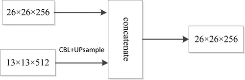
In the prediction network, the Tiny YOLOv3 uses the upsampling to extract feature and strengthen the feature fusion. In Figure 1, the 13 × 13 feature map passes the convolution layer and upsampling layer. This turns the 13 × 13 × 512 feature map into 26 × 26 × 256. The feature map of 26 × 26 also is taken from the earlier in the network and merged with the upsampling feature by concatenation. Finally, the output feature map of 26 × 26 is formed.

Figure 1. The feature fusion of the 26 feature map.

Tiny YOLOv3 divides the input image into N × N grids and predicts the bounding boxes within each grid cell, and the target is detected. Finally, the bounding boxes and confidence for each classification of targets are proposed. The formula is (1) $\begin{array}{r}{C}_i^j=P_r\left(\text{object}\right)\ast {\text{IoU}}_{\text{pred}}^{\text{truth}}\end{array}$(1) where $C_i^j$ refers to the $j$ bounding box of $i$ grid cell, $P_r\left(\text{object}\right)$ is the existence probability of the object . The intersection over union (IoU) is defined as follows: (2) $\begin{array}{r}\text{IoU}=\frac{\text{inter\_area}}{\text{union\_area}}=\frac{B\cap B^{gt}}{B\cup B^{gt}}\end{array}$(2) where, $B^{gt}=(x^{gt},y^{gt},w^{gt},h^{gt})$ represents the position of the ground-truth, and $B=(x,y,w,h)$ represents the position of the predict box. Therefore, the IoU loss function is suggested to be adopted for the IoU metric. (3) $\begin{array}{r}{L}_{\text{IoU}}\text{ = }1-\frac{|B\cap B^{gt}|}{|B\cup B^{gt}|}\end{array}$(3) The loss function of the Tiny YOLOv3 is defined from three aspects: the bounding box position error, the bounding box confidence error and the classification prediction error between the ground truth and the predicted boxes. (4) $\begin{array}{rl}\text{Loss}& ={\lambda }_{\text{coord}}\sum _{i=0}^{s^2}\sum _{j=0}^B{l}_{ij}^{\text{obj}}\left[{(x_i+{\hat{x}}_i)}^2+{(y_i-{\hat{y}}_i)}^2\right]\\ & +{\lambda }_{\text{coord}}\sum _{i=0}^{s^2}\sum _{j=0}^B{l}_{ij}^{\text{obj}}\\ & \times \left[{(\sqrt{w_i}+\sqrt{\widehat{w_i}})}^2+{(\sqrt{h_i}+\sqrt{{\hat{h}}_i})}^2\right]\\ & +{\lambda }_{\text{coord}}\sum _{i=0}^{s^2}\sum _{j=0}^B{l}_{ij}^{\text{noobj}}{(C_i-{\hat{C}}_i)}^2\\ & +{\lambda }_{coord}\sum _{i=0}^{s^2}\sum _{j=0}^B{l}_{ij}^{\text{obj}}{(C_i-{\hat{C}}_i)}^2\\ & +\sum _{i=0}^{s^2}{l}_{ij}^{\text{obj}}\sum _{(c\in \text{class})}{\left(P_i\right(c)-{\hat{P}}_i\left(c\right))}^2\end{array}$(4) where ${\lambda }_{\text{coord}},{\lambda }_{\text{noobj}}$ are the weight parameters and given in advance, the latter is much smaller than the former. $(x_i,y_i,w_i,h_i)$ is the predicted bounding boxes after normalization. $({\hat{x}}_i,{\hat{y}}_i,{\hat{w}}_i,{\hat{h}}_i)$is the ground truth boxes after normalization. $l_{ij}^{\text{obj}}$ determines whether the $j$ bounding box in the $i$ cell grid contains an object. In the Equation (4), the first line represents position and shows that the difference between the actual encoded position of the box and the predicted. And ${\lambda }_{\text{coord}}\sum _{i=0}^{s^2}\sum _{j=0}^B{l}_{ij}^{\text{noobj}}{(C_i-{\hat{C}}_i)}^2$ represents the confidence of no object bounding box, while ${\lambda }_{\text{coord}}\sum _{i=0}^{s^2}\sum _{j=0}^B{l}_{ij}^{\text{obj}}{(C_i-{\hat{C}}_i)}^2$ represents the confidence of the object bounding box. The second line represents the prediction of the confidence box which is the comparison of the confidence value in the actual box prediction results with 1. The third line represents the classification error between the results of predicted and ground truth. In addition, $l_{ij}^{\text{obj}}$ determines that any object central point falls in the cell grid (Figure 2).

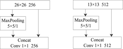
Figure 2. The maxpooling and concatenation of the two scale.

2.2. Enhance feature fusion

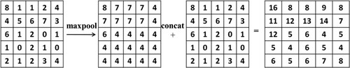
In the maxpooling, the main features are preserved while the parameters and calculation amount are reduced to prevent overfitting and improve the generalization ability of the model. SPP-net uses three different scales for maxpooling. So, the improved Tiny YOLOv3 is based on the SPP-net, it cuts the pooling scale reduces the data processing. But only the maxpooling layer of 5 × 5 is retained. It can greatly increase the receptive field and isolate the most significant contextual features. So an approach is proposed in the improved Tiny YOLOv3 to effectively extract features. The two feature maps are separately made by combining the maxpooling layer. And the pooling kernel is 5 × 5 with the convolution layer with the convolution kernel is 1 × 1. As shown in Figure 3, the maxpooling with 5 × 5 filters and 1 stride. It can greatly increase the receptive field and isolate the most significant contextual features.

Figure 3. The specific implementation of the maxpooling and concatenation.

In the PANet, bottom-up path augmentation is created to shorten information path and enhance feature pyramid with accurate localization signals existing in low-levels. Then, the PANet develops the adaptive feature pooling to recover broken information path between each proposal and all feature levels. This repeated extraction of features and the increase of feature fusion are conducive to better detection of targets. However, the Tiny YOLOv3 only passes the output feature map of 26 × 26 by convolution and concatenation to enhance the feature fusion. Inspired by the principles and observations of the PANet, we propose a new structure, which adds an output feature map of 13 × 13 by upsample to enhance the feature fusion. It proposes the feature map size of 13 × 13 to upsample and downsample the feature map size of 26 × 26, in order to enhance the feature fusion. 26 × 26 feature map passes the zeropadding layer and the convolution layer. This turns the 26 × 26 × 256 feature map into 13 × 13 × 512. We also take a feature map of 13 × 13 from earlier in the network and merge it with the zeropadding features using concatenation. Finally, the output feature map of 13 × 13 is formed. Figure 4 shows the above process.

Figure 4. The output feature map of the 13 × 13 feature scale.

2.3. Improved extraction network

Based on the existing Tiny YOLOv3 network, an improved Tiny YOLOv3 network structure is proposed. In the trunk network, the single-scale maxpooling layer and concatenation and convolution is added to screen the main features and reduce the parameters, and the convolution layer is used to strengthen network and extract the deeper features. The improved Tiny YOLOv3 passes the output feature map of 13 × 13 and 26 × 26 to enhance the feature fusion. By using an input image of 416, the improved Tiny YOLOv3 gets the output feature scales of 13 × 13 and 26 × 26. The improved Tiny YOLOv3 could improve the accuracy of object detection and can detect objects in real-time. The network structure diagram is shown in Figure 5, and the part marked in red is where the improved Tiny YOLOv3 has improved it however the Tiny YOLOv3 did not have that part.

Figure 5. The network structure of the improved Tiny YOLOv3.

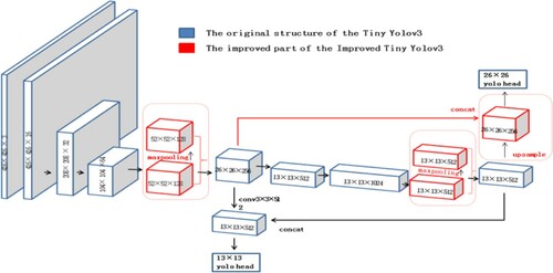
Table 1 lists the different convolution neural network module size. The module size of the YOLOv3 is 246.5M, and the module size of the Tiny YOLOv3 is 33.2M. However, the module size of the improved Tiny YOLOv3 is 55.9M. It is similar to the Tiny YOLOv3, and it is much smaller than YOLOv3. Therefore, the improved Tiny YOLOv3 is also suitable for the real-time detection and other lightweight processors likes FPGA.

Table 1. Different network model size.

Algorithm name	Module size/M
YOLOv3	246.5
Tiny YOLOv3	33.2
Improved TinyYOLOv3	55.9

2.4. Improved loss function

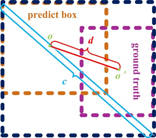
IoU loss function only considers the overlap rate. So, there is an inevitable downside to using IoU loss function for optimization. It only works when the bounding boxes have overlap, and any moving gradient for non-overlapping cases would not be provided. The distance-IoU (DIoU) loss adds a penalty item on the basis of the IoU loss function, which is used to minimize the distance between the central points of two bounding boxes. However, the bounding boxes have three elements: the overlap rate, the central point distance and the aspect ratio. The CIoU loss function is based on the DIoU function. Then the consistency of aspect ratio is imposed to the CIoU loss function to solve this problem.

In Figure 6, $c$ represents the diagonal distance of the minimum closure area that contains both the prediction box and the ground truth, where b and b^gt denote the central points of B and $B^{gt}$, ρ(·) is the Euclidean distance, and c is the diagonal length of the smallest enclosing box covering the two boxes. As shown in Figure 6, the d is the distance between o and o′, and the o is the central of the predict box, and $o^{\mathrm{\prime }}$ is the central of the ground truth. (5) $\begin{array}{r}{R}_{\text{CIoU}}=\frac{{\rho }^2(b,b^{gt})}{c^2}+\alpha \nu \end{array}$(5) where $\alpha$ is the positive trade-off parameter, and $v$ measures the consistency of aspect ratio. The $\alpha$ is defined as (6) $\begin{array}{r}\alpha =\frac{\nu }{1-\text{IoU}+\nu }\end{array}$(6) The $\nu$ is defined as (7) $\begin{array}{r}\nu =\frac{4}{{\pi }^2}(\arctan \frac{{\omega }^{gt}}{h^{gt}}-\arctan \frac{\omega }{h}{)}^2\end{array}$(7) where $\frac{{\omega }^{gt}}{h^{gt}}$ represents the aspect ratio of the prediction box, $\frac{\omega }{h}$ represents the aspect ratio of the real box. The loss function is be defined as (8) $\begin{array}{r}Los{s}_{\text{CIou}}=1-\text{CIoU}=1-\text{IoU}+\frac{{\rho }^2(b,b^{gt})}{c^2}+\alpha \nu \end{array}$(8) The $\frac{\mathrm{\partial }v}{\mathrm{\partial }w}$ and $\frac{\mathrm{\partial }v}{\mathrm{\partial }h}$ should be specified (9) $\begin{array}{rl}\frac{\mathrm{\partial }v}{\mathrm{\partial }w}& =\frac{8}{{\pi }^2}(\arctan \frac{w^{gt}}{h^{gt}}-\arctan \frac{w}{h})\times \frac{h}{w^2+h^2}\\ & \times \frac{\mathrm{\partial }v}{\mathrm{\partial }h}=\frac{8}{{\pi }^2}(\arctan \frac{w^{gt}}{h^{gt}}-\arctan \frac{w}{h})\times \frac{w}{w^2+h^2}\end{array}$(9) where $w^2+h^2$ is a small value for the cases $h$ and $w$ ranging in [0, 1] to yield gradient explosion. Compared with the IoU loss function, CIoU loss function not only has the same overlap rate as the IoU loss function, but also has the central point distance and the aspect ratio that it does not have. In a nutshell, the CIoU loss function makes the bounding boxes regression more stable.

Figure 6. The CIoU loss function for bounding box regression.

2.5. K-means clustering

K-means is a partition-based clustering method and usually used to find the optimal number and size of anchor boxes. It takes the sum of squared errors as the objective function to measure clustering quality, by calculating the distance between each data object with the central of K’s cluster, divide the data into the closest classification, then it will adjust the cluster central and iterate until the cluster central no longer change. The Euclidean distance function is used by traditional K-means clustering method, but the larger boxes have more error clustering than smaller in this method. Therefore, the distance of the improved Tiny YOLOv3 adopted IoU function, the distance function is the following formula: (10) $\begin{array}{r}\text{distance}\left(\text{box,centroid}\right)=1-\text{IoU(box,centroid})\end{array}$(10) where $\text{box}$ represents the collection of the ground truth, $\text{centroid}$ represents the cluster central collection of the bounding boxes, and the $\text{IoU(box,centroid)}$ represents the ratio of the intersection and union of the cluster central of the ground truth and the bounding boxes. However, the higher the IoU is, the higher the correlation and the closer the two boxes are. There are three anchors in every size of feature map. And it is two size feature maps of the improved Tiny YOLOv3. Six cluster values are calculated by training the dataset, and they respectively are (36, 75), (76, 55), (72, 146), (142, 110), (192,243), (459, 401).

3. Experimental results

3.1. Experiment environment

The training experimental environment of the improved Tiny YOLOv3 is implemented in a Python library which called Keras, and the Keras is running on the top of TensorFlow. The experiment is trained in the environment of CPU. The total iteration number is 50, the initial learning rate is 0.001, the batch input quantity is 1, the weight attenuation coefficient is 0.0001, and the patience is 3.

3.2. Image dataset creation

The improved Tiny YOLOv3 uses the self-made dataset. We collect 400 pictures of setscrews and nuts on the conveyor belt, the objects of dataset are marked by using LabelImage software, which can generate the position and classification of the object in training files. There are two classifications of sample in dataset called setscrew and nut. It represents the big object and small object respectively. The real-time detection on the conveyor belt is the detection of the classification and moving objects. To prevent the overfitting, 70% of the dataset are used for training, 10% for validation, and 20% for testing.

3.3. Experimental results and analysis

3.3.1. The method for calculating precision

The dataset is trained and tested in the Tiny YOLOv3 and the improved Tiny YOLOv3. Precisions and recall are usually used to evaluate network performance. And the precisions and recall of each classification in different method are calculated. (11) $\begin{array}{r}\text{Precision}=\frac{\text{TP}}{\text{TP + FP}},\text{Recall}=\frac{\text{TP}}{\text{TP + FN}}\end{array}$(11) where $\text{TP}$ represents the true positive, $\text{FP}$ represents the false positive, and $\text{FN}$ represents the false negative. The average precision (AP) is the area of a graph includes precisions and recall, and the mAP is the mean area of the whole graphs.

3.3.2. The module size and detection speed of the algorithm

As shown in Table 2. For detection speed in GPU running, the fps of Tiny YOLOv3 is 35.5, and the fps of improved Tiny YOLOv3 is 32.5. Though the algorithm proposed in this paper detection speed in GPU is slower 3 fps than Tiny YOLOv3, it still meets the requirements of real-time detection. Because the network structure of improved Tiny YOLOv3 is a little bigger than Tiny YOLOv3.

Table 2. Detection speed of different algorithms.

Algorithm name	GPU fps/(frames·${\text{s}}^{-1}$)	CPU fps/(frames·${\text{s}}^{-1}$)
Tiny YOLOv3	35.5	1.2
Improved Tiny YOLOv3	32.5	1.1

3.3.3. The precision of different algorithms

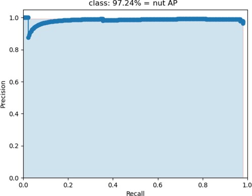
The detection result is shown in Figures 7–10. Figure 7 shows the setscrew AP of the Tiny YOLOv3 is 90.76%, and the nut AP of the Tiny YOLOv3 is 32.18% in Figure 8. In Figure 9, it shows the setscrew AP of the improved Tiny YOLOv3 is 93.88%, whereas Figure 10 shows the nut AP of the improved Tiny YOLOv3 is 97.24%.

Figure 7. The setscrew AP of Tiny YOLOv3.

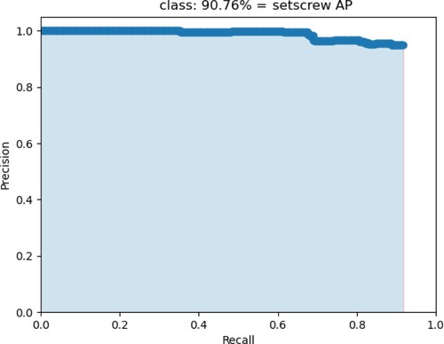
Figure 8. The nut AP of Tiny YOLOv3.

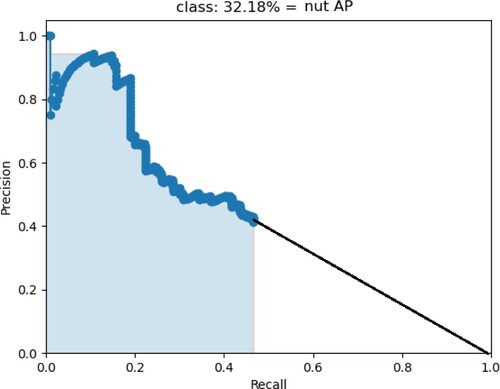
Figure 9. The setscrew AP of improved Tiny YOLOv3.

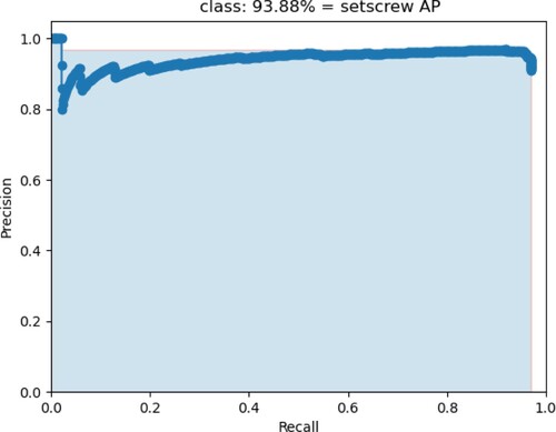
Figure 10. The nut AP of improved Tiny YOLOv3.

In Table 3, the AP of the improved Tiny YOLOv3 is higher than Tiny YOLOv3, whatever classification is setscrew or nut, especially in the detection of nut. In the detection of setscrew, the improved Tiny YOLOv3 is 3.12% higher than Tiny YOLOv3. In the detection of nut, the improved Tiny YOLOv3 is 65.06% higher than Tiny YOLOv3. According to this result, the improved Tiny YOLOv3 can better detect the objects especially in the small objects.

Table 3. The average precision of the different classification.

Algorithm name	Class	AP (%)
Tiny YOLOv3	Setscrew	90.76
Tiny YOLOv3	Nut	32.18
Improved Tiny YOLOv3	Setscrew	93.88
Improved Tiny YOLOv3	Nut	97.24

Figures 11 and 12 show the mAP of the Tiny YOLOv3 and improved Tiny YOLOv3. In Figure 11, the mAP of Tiny YOLOv3 is 61.47%, whereas the mAP of improved Tiny YOLOv3 is 95.56% in Figure 12. The mAP of improved Tiny YOLOv3 is more than Tiny YOLOv3. And the reason is that the improved Tiny YOLOv3 has a better network structure for extracting image features and uses CIoU loss function.

Figure 11. The mAP of Tiny YOLOv3.

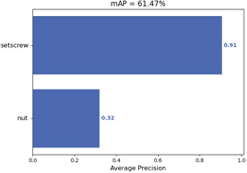
Figure 12. The mAP of improved Tiny YOLOv3.

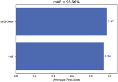
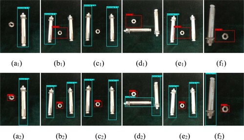
Figure 13 is the real scene detection result of the Tiny YOLOv3 algorithm and improved Tiny YOLOv3 algorithm. (a₁)–(d₁) in Figure 13 is the detection results of the Tiny YOLOv3, and (a₂)–(d₂) in Figure 13 is the detection results of improved Tiny YOLOv3 in the same scene. (e₁) and (e₂) shows the two different detection algorithm results of 30% increase under the current illumination, (f₁) and (f₂) shows the detection result of 30% reduce under current illumination. In detection results of the (a₁) and (c₁), nuts are missed. In the (b₁), (d₁) and (e₁), the setscrews also are missed. No matter how the illumination changes, in the detection algorithm of improved Tiny YOLOv3 all the objects are detected. From the detection results, the improved Tiny YOLOv3 has a good adaptation to the complex illumination variation, and it can detect the object much more accurate than the Tiny YOLOv3 in real-time detection (Figure 13).

Figure 13. The comparison diagram of experimental results.

4. Conclusion

The improved Tiny YOLOv3 enhances the extraction network, and the feature fusion also is strengthened by upsampling and downsampling in two feature map layers. What’s more, the improved Tiny YOLOv3 revised the IoU to CIoU in the loss function. All about this improves the detection accuracy. Although the network model of the improved Tiny YOLOv3 is grown, the accuracy has improved dramatically comparing to the Tiny YOLOv3. The detection speed of improved Tiny YOLOv3 is not slow down so much, and it can be trained in CPU. However, it can still meet the requirement of real-time detection and can be run on small processors like FPGA. After training and testing the dataset, the obtained experiment result shows that the mAP of object detection of improved Tiny YOLOv3 is 95.56%. It’s 34.09% better than the Tiny YOLOv3 in the same sense. In GPU, the fps of the improved Tiny YOLOv3 is 35.5 fps. It is about 3 frames less than the Tiny YOLOv3, but it can still meet the requirements of real-time detection. And the next work is that reducing the size of the model while maintaining the detection accuracy.

Acknowledgements

This work is supported by National Nature Science Foundation under Grant 61603220, 61733009; the Research Fund for the Taishan Scholar Project of Shandong Province of China; SDUST Young Teachers Teaching Talent Training Plan under Grant BJRC20180503, BJRC20190504.

Disclosure statement

No potential conflict of interest was reported by the author(s).

Additional information

Funding

This work was supported by National Natural Science Foundation [grant numbers 61603220, 61733009]; the Research Fund for the Taishan Scholar Project of Shandong Province of China; SDUST Young Teachers Teaching Talent Training Plan [grant numbers BJRC20180503, BJRC20190504].

References

- Dollar, P., Appel, R., & Belongie, S. (2014). Fast feature pyramids for object detection. IEEE Transactions on Pattern Analysis and Machine Intelligence, 36(08), 1532–1545. https://doi.org/https://doi.org/10.1109/TPAMI.2014.2300479
- Girshick, R. (2015, 13–16 December). Fast r-cnn. 2015 IEEE International Conference on Computer Vision (ICCV), Santiago (pp. 1440–1448).
- Girshick, R., Donahue, J., & Darrell, T. (2014, 23–28 June). Rich feature hierarchies for accurate object detection and semantic segmentation. Proceedings of the IEEE Conference on Computer Vision and Pattern Recognition, Columbus (pp. 580–587).
- He, K. M., Gkioxari, G., Dollár, P. & Girshick, R. (2017, 22–29 October). Mask R-CNN. In IEEE international conference on computer vision (ICCV), Venice (pp. 386–397).
- He, K. M., Zhang, X. Y., & Ren, S. Q. (2015). Spatial pyramid pooling in deep convolutional networks for visual recognition. IEEE Transactions on Pattern Analysis and Machine Intelligence, 37(9), 1904–1916. https://doi.org/https://doi.org/10.1109/TPAMI.2015.2389824
- He, K., Zhang, X., Ren, S. & Sun, J. (2016, 27–30 June). Deep residual learning for image recognition. In Proceedings of the IEEE conference on computer vision and pattern recognition, Las Vegas (pp. 770–778).
- Liu, W., Anguelov, D., & Erhan, D. (2016). SSD: Single shot multibox detector. Computer Vision - ECCV 2016, PT I. Lecture Notes in Computer Science, 9905, 21–37. https://doi.org/https://doi.org/10.1007/978-3-319-46448-0_2
- Manju, A., & Valarmathie, P. (2020). Video analytics for semantic substance extraction using opencv in python. Journal of Ambient Intelligence and Humanized Computing. https://doi.org/https://doi.org/10.1007/s12652-020-01780-y
- Mazzia, V., Khaliq, A., & Salvetti, F. (2020). Real-time apple detection system using embedded systems with hardware accelerators: An edge AI application. IEEE ACCESS, 08, 9102–9114. https://doi.org/https://doi.org/10.1109/ACCESS.2020.2964608
- Redmon, J., Divvala, S., & Girshick, R. (2016, 27–30 June). You only look once: Unified, real-time object detection. In Proceedings of the IEEE conference on computer vision and pattern recognition, Las Vegas (pp. 779–788).
- Redmon, J., & Farhadi, A. (2017, 21–26 July). YOLO9000: better, faster, stronger. In Proceedings of the IEEE conference on computer vision and pattern recognition, Honolulu (pp. 6517–6525).
- Redmon, J., & Farhadi, A. (2018). YOLOv3: An incremental improvement. arXiv Preprint arXiv, 1804.02767.
- Ren, S. Q., He, K. M., & Girshick, R. (2017). Faster R-CNN: Towards real-time object detection with region proposal networks. IEEE Transactions on Pattern Analysis and Machine Intelligence, 39(6), 1137–1149. https://doi.org/https://doi.org/10.1109/TPAMI.2016.2577031
- Tian, Y., Yang, G. D., & Wang, Z. (2019). Apple detection during different growth stages in orchards using the improved YOLOv3 model. Computers and Electronics in Agriculture, 157, 417–426. https://doi.org/https://doi.org/10.1016/j.compag.2019.01.012
- Wachs, J. P., Stern, H. I., & Burks, T. (2010). Low and high-level visual feature-based apple detection from multi-modal images. Precision Agriculture, 11(06), 717–735. https://doi.org/https://doi.org/10.1007/s11119-010-9198-x
- Zhang, Y., Shen, Y. L., & Zhang, J. (2019). An improved Tiny YOLOv3 pedestrian detection algorithm. OPTIK, 183, 17–23. https://doi.org/https://doi.org/10.1016/j.ijleo.2019.02.038