Application of a noise reduction method combining AVMD and SVD in natural gas pipeline leakage signal

Abstract

Due to the large amount of noise in pipeline leakage signal, the accuracy of the leakage detection device's judgment will be reduced by direct leakage detection. Therefore, the noise reduction of pipeline leakage signal is critical for preprocessing technology of pipeline leakage detection. A denoising method combining adaptive variational mode decomposition (AVMD) and singular value decomposition (SVD) is proposed in this paper. First, the mode number and the penalty factor of VMD are searched automatically by AVMD. The AVMD algorithm is coupled to a fitness function based on improved refine composite multiscale dispersion entropy (RCMDE). Subsequently, a time–frequency matrix which obtains time–frequency subspace after SVD is constructed for all mode components decomposed by VMD, and the number of effective time–frequency subspaces is determined by the relative change rate of singular values, thereby the denoised signal is achieved. Finally, the experimental results show that the AVMD-SVD method proposed in this paper has the significant denoising effect and strong robustness.

KEYWORDS:

• Variational mode decomposition
• parameter optimization
• signal denoising
• pipeline leakage

1. Introduction

Pipeline is the main mode of transportation for large quantities of natural gas. For long-distance transportation, the pipeline is very cost-effective because it has the advantages of low cost, safety and so on (Muggleton et al., 2020). However, pipeline leakage occurs frequently because of aging, corrosion, and other forms of damage, which poses a great threat to the safe transportation of pipelines (Zhang et al., 2014). Pipeline leakage has a series of adverse effects on the environment, economy, health, and safety. In view of the above facts, accurate detection and early warning of leakage pipelines are very necessary and significant (Liu et al., 2017). The main methods to solve pipeline leakage include: acoustic wave method (Xiao et al., 2019), negative pressure wave detection method (Li, Zheng, et al., 2019), transient model method (Murvay & Silea, 2012), distributed optical fibre method (Muggleton et al., 2020). Considering that the acoustic method has higher sensitivity and stronger adaptability than traditional methods, a lot of research on it have been conducted by experts and scholars. In Liang et al. (2013), the sound principle and source characteristics of pipeline leakage have been studied, then a novel acoustic technology for pipeline leakage detection model has been proposed. In Liu et al. (2015), a leakage detection and location method based on propagation law has been proposed by studying propagation law of attenuation and using correction factor to correct the actual propagation model. However, due to the influence of the complex environment during pipeline transportation, a large amount of noise is mixed into the acoustic signal. Therefore, effectively filtering out the noise in the pipeline leakage signal is of great significance to pipeline leakage detection technology.

In practice, various methods of signals denoising have been investigated. The wavelet transform (WT) method is a practical tool for signal denoising, and it has a wide range of applications in various fields (Huang et al., 2018; Xin et al., 2020). Given that WT has good time–frequency characteristics, nonlinear signal can be denoised effectively. The selection of the mother wavelet and the number of decomposition layers are closely related to the extracted feature information, which is crucial to the denoising performance. The empirical mode decomposition (EMD) (Huang et al., 1998) is a method of adaptively signal decomposition. Lahmiri and Boukadoum (2015) has been decomposed the bio-signal by EMD, assigned a specific weight to each IMF obtained and passed the discrete wavelet transform (DWT) threshold to reduce noise. However, the end effect problem of EMD and the mode aliasing phenomenon need to be optimized. In 2014, Dragomiretskiy and Zosso (2014) proposed variational mode decomposition (VMD). As a new signal decomposition method, the VMD algorithm could overcome the problems of endpoint effects and modal aliasing. Furthermore, VMD makes up for the shortcomings of EMD and has good stability and robustness. If the parameter values $\left[K,\alpha \right]$ of VMD are not set properly, it may cause under-decomposition or over-decomposition. In Yang et al. (2019), the simulated annealing (SA) algorithm has been applied to search for the control parameters of VMD. In Zhang et al. (2018), a method for optimizing the parameter values has been proposed by the grasshopper optimization algorithm (GOA). In Yi et al. (2016), the improved cross-correlation coefficient has been used as the fitness function of the particle swarm optimization (PSO) algorithm, and then the parameters of VMD have been optimized by PSO. In Gu et al. (2020), the grey wolf optimization algorithm (GWOA) using the minimum average envelope entropy as the fitness function has been optimized the control parameters adaptively. This method could accurately identify the frequency of the fault feature. In Lu et al. (2020), VMD has been used in combination with the Bhattacharyya distance based on variance method to optimize the modes. In Li et al. (2020), the maximum envelope kurtosis has been used as an index for optimizing and determining the number of VMD modes. In Zhou and Zhu (2019), an algorithm combining VMD and singular spectrum analysis (SSA) has been used to filter seismic noise. In Zhou et al. (2020), a multi-feature fusion method has been proposed to extract the characteristics of pipeline signal. The effective characteristic parameters have been selected to form the characteristic vector and the support vector machine (SVM) has been used to identify the different pipeline signals. The two-dimensional variational mode decomposition (2D-VMD) and the Hausdorff distance (HD) in Gao et al. (2020) has been presented to denoising oil and gas pipeline images. Singular value decomposition (SVD) is an effective signal denoising method. In Zhao and Jia (2017), in order to extract weak features caused by early failures, a reweighted SVD strategy has been proposed for denoising signal and enhancing the weak feature of signal. In Zhang et al. (2017), higher-order SVD has been investigated to the denoising of diffusion-weighted images. In Li, liu, et al. (2019), a new type of relative change rate of singular value kurtosis (SVK) has been proposed to determine the reconstruction order of singular values.

For the interference brought by artificially set VMD parameters on signal decomposition, a signal denoising method based on the combination of AVMD and SVD has been proposed in this paper. First, input the parameter pair $\left[K,\alpha \right]$ adaptively optimized by the AVMD algorithm into VMD, and decompose a series of intrinsic mode functions (IMFs) for the noise signal. Second, the time–frequency matrix composed of $K$ mode components is subjected to SVD processing. Subsequently, the effective IMFs are selected to reconstruct the signal through the relative change rate of singular values to achieve signal denoising. Finally, the combined method of AVMD and SVD proposed in this paper is used to de-noise the simulation signal and the pipeline leakage signal, respectively. The main contributions of this paper are summarized as follows: (1) the AVMD algorithm is proposed to optimize the mode component number $K$ and penalty factor $\alpha$ of VMD adaptively, so as to avoid the inaccuracy of setting parameters artificially; (2) the improved refine composite multiscale dispersion entropy (RCMDE) is used as the fitness function of the AVMD method and (3) the combination of AVMD and SVD (AVMD-SVD) is applied to denoise the natural gas pipeline leakage signal.

The rest of this paper is arranged as follows. Section 2 states the basic mechanism of VMD and the novel fitness function based on RCMDE, as well as the SVD. Section 3 introduces the AVMD method and AVMD-SVD joint noise reduction method. In Section 4, the simulated and real leakage signal are used to validate the AVMD method, the robustness and superior of the proposed are demonstrated by comparing with several of optimizing parameters methods. In Section 5, the conclusions are summarized.

2. Theoretical basis

2.1. Theory of VMD

The VMD algorithm can decompose the signal $f\left(t\right)$ into $K$ sub-modes, each mode component has its corresponding centre frequency $\omega \left(t\right)$. This method can estimate the frequency bandwidth of each mode component. The specific steps are listed as follows:

1. The analytic signal of each mode component is obtained by Hilbert transform, and then its marginal spectrum is solved.

2. For each mode component, the centre frequency of the mode is estimated according to the exponential hybrid modulation, and the spectrum of the mode is moved to the ‘baseband’.

3. The bandwidth of each mode function is estimated by the Gaussian smoothness and gradient square criterion of demodulation signal. The VMD constrained variational expression obtained through the above steps is given as follows: (1) $\begin{array}{rl}& \underset{\left\{u_k,{\omega }_k\right\}}{min}\left\{\sum _k{∥{\mathrm{\partial }}_t\left[\left(\delta \left(t\right)+\frac{j}{\pi t}\right)\ast u_k\left(t\right)\right]e^{-j{\omega }_{k}t}∥}_2^2\right\}\\ & s.t.\sum _k{u}_k=f\end{array}$(1) where $\left\{u_k\right\}=\left\{u_1,u_2,\dots ,u_K\right\}$ represents the decomposition of signal $f\left(t\right)$ into a set of $K$ IMFs. $\left\{{\omega }_k\right\}=\left\{{\omega }_1,{\omega }_2,\dots ,{\omega }_K\right\}$ is the set of centre frequencies of the decomposed components. $\delta \left(t\right)$ represents the unit impulse function. ${\mathrm{\partial }}_t$ represents the partial derivative concerning for to $t$. ${\sum }_k={\sum }_{k=1}^K$ represents the sum of all mode components.

The quadratic penalty factor $\alpha$ and Lagrange multiplication operator $\lambda$ are used to construct the augmented Lagrange function to transform the above-mentioned constrained variational problem into an unconstrained variational problem, which is specifically expressed as follows: (2) $\begin{array}{rl}& L\left(\left\{u_k\right\},\left\{{\omega }_k\right\},\lambda \right)\\ & =\alpha \sum _k{∥{\mathrm{\partial }}_t\left[\left(\delta \left(t\right)+\frac{j}{\pi t}\right)\ast u_k\left(t\right)\right]e^{-j{\omega }_{k}t}∥}_2^2\\ & +{∥f\left(t\right)-\sum _k{u}_k\left(t\right)∥}_2^2+〈\lambda \left(t\right),f\left(t\right)-\sum _k{u}_k\left(t\right)〉\end{array}$(2)

The Lagrange function of the Equation (2) is transformed into the frequency domain. The frequency domain expressions of the mode component $u_k$ and the centre frequency ${\omega }_k$ are described as follows: (3) $\begin{array}{rl}{\hat{u}}_k^{n+1}\left(\omega \right)& =\frac{\hat{f}\left(\omega \right)-{\sum }_{i\ne k}{\hat{u}}_i\left(\omega \right)+\frac{\hat{\lambda }\left(\omega \right)}{2}}{1+2\alpha {\left(\omega -{\omega }_k\right)}^2}\end{array}$(3) (4) $\begin{array}{rl}{\omega }_k^{n+1}& =\frac{{\int }_0^{\mathrm{\infty }}\omega {|{\hat{u}}_k\left(\omega \right)|}^{2}d\omega }{{\int }_0^{\mathrm{\infty }}{|{\hat{u}}_k\left(\omega \right)|}^{2}d\omega }\end{array}$(4)

1. Using the Alternate Direction Method of Multipliers (ADMM) algorithm to perform a series of iterative optimizations to find the ‘saddle point’ of Equation (2) is the optimal solution of Equation (1), thereby decomposing the signal $f\left(t\right)$ into $K$ IMFs. The implementation steps of the $u_k$ are described as follows:

  Step 1: Initialization $\left\{u_k^1\right\},\left\{{\omega }_k^1\right\},{\hat{\lambda }}^1,n\leftarrow 0$;

  Step 2: $n=n+1$, starting loop;

  Step 3: For $k=1:K$ do;

Update ${\hat{u}}_k$: (5) ${\hat{u}}_k^{n+1}\left(\omega \right)\leftarrow \frac{\begin{array}{c}\hat{f}\left(\omega \right)-{\sum }_{i<k}{\hat{u}}_i^{n+1}\left(\omega \right)\\ -{\sum }_{i>k}{\hat{u}}_i^n\left(\omega \right)+\left({\hat{\lambda }}^n\right(\omega \left)/2\right)\end{array}}{1+2\alpha {\left(\omega -{\omega }_n^k\right)}^2}$(5)

Update ${\omega }_k$: (6) ${\omega }_k^{n+1}\leftarrow \frac{{\int }_0^{\mathrm{\infty }}\omega {|{\hat{u}}_k^{n+1}\left(\omega \right)|}^{2}d\omega }{{\int }_0^{\mathrm{\infty }}{|{\hat{u}}_k^{n+1}\left(\omega \right)|}^{2}d\omega }$(6)

• Step 4: Double promotion for all $\omega \ge 0$: (7) ${\hat{\lambda }}^{n+1}\left(\omega \right)\leftarrow {\hat{\lambda }}^n\left(\omega \right)+\tau \left(\hat{f}\left(\omega \right)-\sum _k{\hat{u}}_k^{n+1}\left(\omega \right)\right)$(7)

• Step 5: Repeat step 2- step 4 until the iteration stop condition is met: (8) ${\sum }_k{||{\hat{u}}_k^{n+1}-{\hat{u}}_k^n||}_2^2/||{\hat{u}}_k^n|{|}_2^2<ϵ$(8) where $ϵ>0$ is the discrimination accuracy, ${\hat{u}}_k$ and ${\omega }_k$ are obtained at the end of the loop, $K$ IMFs with limited bandwidth are obtained by inverse Fourier transform.

2.2. Fitness function based on RCMDE

Entropy, as an index to measure the uncertainty and complexity of time series, is an effective and widely used method. It could measure the non-linear behaviour of the signal and detect the dynamic changes of weak signal. The RCMDE was proposed by Azami et al. (2017). The RCMDE method has significant advantages in feature extraction, calculation errors, and stability.

The RCMDE is defined as the Shannon entropy of the mean value of the discrete mode of the displacement sequence. The $k^{th}$ coarse-grained time series $X=\left\{x_{k,1}^{\left(\tau \right)},x_{k,2}^{\left(\tau \right)},\dots \right\}$ for the mode component $u$ is described as follows: (9) $x_{k,j}^{\left(\tau \right)}=\frac{1}{\tau }\sum _{b=k+\tau (j-1)}^{k+\tau j-1}{u}_b,1\le j\le N,1\le k\le \tau$(9)

For each scale factor $\tau$, RCMDE is defined as follows: (10) $RCMDE\left(x,m,c,d,\tau \right)=-\sum _{\pi =1}^{c^m}\overline{p}\left({\pi }_{v_0\dots v_{m-1}}\right)\cdot \ln \left(\overline{p}\left({\pi }_{v_0\dots v_{m-1}}\right)\right)$(10) where $\overline{p}\left({\pi }_{v_0\dots v_{m-1}}\right)=\left(1/\tau \right){\sum }_1^{\tau }{p}_k^{\left(\tau \right)}$ with the relative frequency of the dispersion pattern $\pi$ in the series $x_k^{\left(\tau \right)}$. The parameters to be set are: embedding dimension $m=3$, category $c=6$, delay $d=1$, and maximum scale factor ${\tau }_{max}=15$. For more information about parameters, see reference Rostaghi and Azami (2016). This refined method of signal processing may reduce information loss effectively and calculation deviation. RCMDE can measure the complexity of the signal. The lower the complexity, the smaller the value of RCMDE. Calculate the RCMDE for each mode component obtained by VMD, that is, 15 entropy values of different scales, and take the variance of the entropy values (VRCMDE). When VRCMDE has a larger value, the mean value of VRCMDE will have a larger value, indicating that the effective components and the noise components can be separated. Equation (12) is the fitness function of the AVMD algorithm. The specific definitions are described as follows: (11) $\begin{array}{rl}\text{VRCMDE}& =\text{var(RCMDE)}\end{array}$(11) (12) $\begin{array}{rl}\text{MVRCMDE}& =\text{mean(VRCMDE)}\end{array}$(12)

2.3. Introduction of SVD

For any dimensional real matrix $A\in R^{m\times n}$, there must be m-order orthogonal matrices $U=\left[u_1,u_2,\dots ,u_m\right]\in R^{m\times m}$ and $V=\left[v_1,v_2,\dots ,v_n\right]\in R^{n\times n}$ satisfy the following formula: (13) $\begin{array}{rl}A& =U\ast S\ast V^T={\lambda }_1{u}_1{v}_1^T+{\lambda }_2{u}_2{v}_2^T+\dots +{\lambda }_q{u}_q{v}_q^T\\ & =\sum _{i=1}^q{\lambda }_i{u}_i{v}_i^T=\sum _{i=1}^q{\lambda }_{i}A{}_i\end{array}$(13) where $S=\left(diag\left({\lambda }_1,{\lambda }_2,\dots ,{\lambda }_q\right),0\right)$,${\lambda }_1,{\lambda }_2,\dots ,{\lambda }_q$ are the singular values of matrix $A$, ${\lambda }_1\ge {\lambda }_2\ge \cdots \ge {\lambda }_q\ge 0$, the rank of matrix $A$:$rank\left(A\right)=q=min\left(m,n\right)$. $A_i=u_i{v}_i^T$ is the sub-matrix.

3. Signal denoising method of AVMD-SVD

3.1. The principle AVMD

In practical applications, the VMD couldn’t decompose adaptively. The number of the decomposition $K$ and penalty factor $\alpha$ are of great importance for decomposing signal by VMD. For under-decomposition: $K$ value is small, and some low-frequency components are regarded as high-frequency components (the $\alpha$ value is small), or the phenomenon of discarding low-frequency components classified as high frequency (the $\alpha$ value is large); for over-decomposition: $K$ value is too large, and several of the modes contain a lot of noise (the $\alpha$ value is small), or mode replication will occur. In this paper, an optimization method is proposed for adaptively optimizing VMD parameters, which searches for the optimal parameter pair $\left[K,\alpha \right]$ automatically. The detailed processes are as follows:

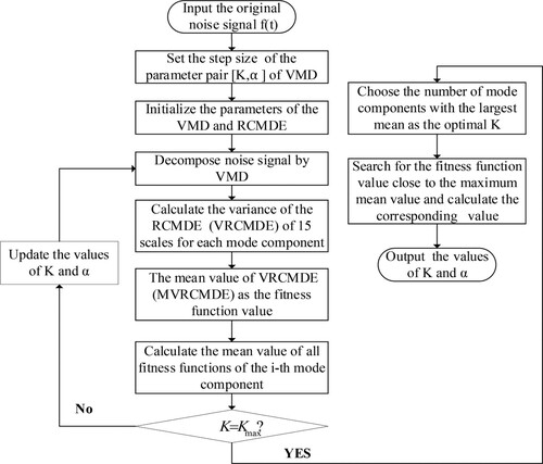
1. Initialize the VMD parameters. Given $K$ value, $\alpha$ value, and the iteration step size. The range of $K$ is an integer of [2,12], and the range of $\alpha$ is [200,6000], and the step size is 50.

2. Set the parameters of RCMDE.

3. Decompose signal by VMD algorithm.

4. The fitness function proposed in this paper is used to iterate the cycle.

5. The fitness function values calculated by the AVMD algorithm are averaged again. That is, calculate the mean value of all fitness function values for each mode component, select the number of mode components corresponding to the largest mean value as the optimal $K$, find the minimum difference between the maximum mean value and the fitness function value, search for the corresponding $\alpha$ value. The formulas for solving the optimal parameters are described as follows: (14) $\begin{array}{rl}\left(\hat{K}\right)& =\underset{\left\{K\right\}}{\arg max}\left(\frac{1}{K}\sum _{i=1}^{K}fitness\left(i\right)\right)\end{array}$(14) (15) $\begin{array}{rl}\left(\hat{\alpha }\right)& =\underset{\left\{\alpha \right\}}{\arg min}{∥fitness\left(i\right)-\frac{1}{\hat{K}}\sum _{i=1}^{\hat{K}}fitness\left(i\right)∥}_2^2\end{array}$(15)

The specific flowchart of the AVMD is shown in Figure 1.

Figure 1. The flowchart of AVMD method optimization parameters.

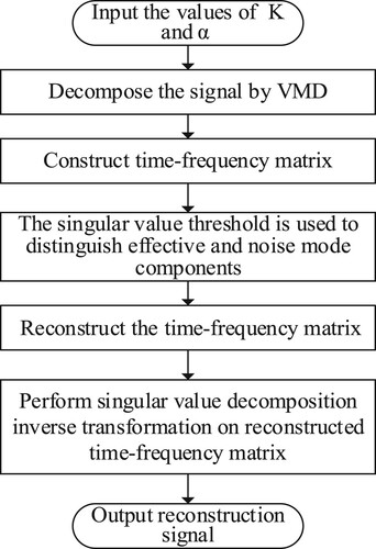
3.2. The AVMD-SVD signal denoising method

SVD is an effective method for signal denoising. In this paper, the signal $x\left(t\right)$ is decomposed by VMD to obtain $K$ IMF components, assuming that the data point of each IMF component is $a_{kn}\left(k=1,2,\cdots ,K;n=1,2,\cdots ,N\right)$, the time–frequency matrix $A$ is expressed as: (16) $A=\left[\begin{array}{cccc}{a}_{11}& a_{12}& \cdots & a_{1n}\\ a_{21}& a_{22}& \cdots & a_{2n}\\ ⋮& ⋮& \ddots & ⋮\\ a_{k1}& a_{k2}& \cdots & a_{kn}\end{array}\right]$(16)

Then, the time–frequency matrix $A$ is subjected to SVD to obtain $K$ time–frequency subspaces and corresponding singular values. The relative change rate of singular values (Wang et al., 2012) is used to determine the number of effective time–frequency subspaces. The inverse singular value transformation of the effective time–frequency matrix is carried out to achieve signal noise reduction. The specific flowchart of the algorithm is as follows Figure 2:

Figure 2. Flowchart based on AVMD-SVD filtering method.

4. Simulation results and analysis

4.1. Simulation test of AVMD-SVD method

In this paper, three different frequency bands of AM and FM signals and a Gaussian white noise signal are combined into a simulation signal to test the accuracy of the AVMD-SVD method. The expression of the simulation signal is following: (17) $\begin{array}{rl}x\left(t\right)& =1.6\sin (2\pi \times f_1\times t)+1.4\cos (2\pi \times f_2\times t)\\ & +1.2\cos (2\pi \times f_3\times t)+\eta \end{array}$(17) where the frequencies of $f_1$,$f_2$,$f_3$ are 2, 20, 200 Hz, respectively. $\eta$ is Gaussian white noise.

The length of the simulated signal is 1024. The experimental results show that the value of RCMDE is smaller, and the complexity of the effective component obtained by VMD decomposition is lower than the noise component. Given that the optimization of the AVMD algorithm is to search randomly, this paper optimizes the parameter pair $\left[K,\alpha \right]$ of VMD for five times. Gaussian white noise with input signal to noise ratio ($SN{R}_{in}$) of 5 and 10 dB is added to the original signal, so as to verify the robustness of AVMD, respectively. It is compared with the VMD parameters optimized by the standard particle swarm optimization (SPSO) algorithm and genetic algorithm (GA) to illustrate the performance of AVMD. The optimization methods all use $fitness$ as the fitness function, and the search range of optimized VMD parameters remains consistent. The optimized parameter pairs of VMD are shown in Tables 1 and 2. The average value of the optimized parameters in the table below is used as the best parameter pair. From Tables 1 and 2, when Gaussian white noise with different $SN{R}_{in}$ is added, the optimal $K$ obtained by AVMD is 4, the variance is small, and there is almost no fluctuation. Since the simulation signal consists of three cosine harmonic signals and a noise component, it can be determined that the VMD parameters optimized by the AVMD method have not been under-decomposition or over-decomposition. The parameter pairs optimized by the SPSO-VMD method with different $SN{R}_{in}$ are [5,2400] and [3,4957], respectively. It can be seen from the variance of the $K$ value that the optimization results fluctuate greatly, and the optimized $\alpha$ value easily falls into the local optimum. The variance of $K$ value optimized by the GA-VMD method is relatively large. Due to the optimized $K$ value differs greatly from the number of mode components of the input signal, over-decomposition may occur. Therefore, the comparison shows that the control parameters of the VMD optimized by the AVMD method proposed in this paper are relatively stable.

Table 1. Optimization results of different methods with $SN{R}_{in}$=5 dB.

$SN{R}_{in}$=5 dB	AVMD		SPSO-VMD		GA-VMD
Sequence number	$K$	$\alpha$	$K$	$\alpha$	$K$	$\alpha$
1	4	3300	5	3072	5	4965
2	4	5850	4	915	8	1698
3	4	800	5	1503	5	1628
4	5	2750	6	4312	5	2866
5	4	3800	4	2196	8	1293
Mean value	4	2260	5	2400	6	2490
Variance	0.2	2.1e+06	0.7	1.8e+06	2.7	2.3e+06

Table 2. Optimization results of different methods with $SN{R}_{in}$=10 dB.

$SN{R}_{in}$=10 dB	AVMD		SPSO-VMD		GA-VMD
Sequence number	$K$	$\alpha$	$K$	$\alpha$	$K$	$\alpha$
1	4	3400	2	5831	9	2958
2	4	4300	4	2747	3	2545
3	4	2300	2	4207	3	4871
4	4	3550	4	6000	9	4110
5	4	3000	4	6000	9	4110
Mean value	4	3310	3	4957	7	3719
Variance	0	5.4 e+05 e+05	1.2	2.1 e+06	10.8	8.9 e+05

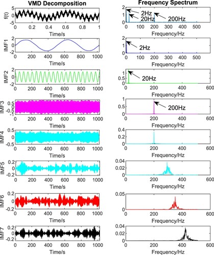
For this purpose, a simulation signal with $SN{R}_{in}$ of 10 dB is taken as an example. The result of the AVMD method to decompose the simulation signal is shown in Figure 3. It can be found that the AVMD method can separate the effective mode components and the noise components completely. The signal is decomposed into 3 effective mode components and 1 noise component. Moreover, the centre frequencies of the effective mode components are 2, 20, and 200 Hz, respectively, which correspond to the frequency of the original signal. There is no phenomenon of under-decomposition or over-decomposition. The result of SPSO optimized VMD is shown in Figure 4. It can be found that VMD decomposes 2 effective mode components and 1 noise component. The mode components with centre frequencies of 2 and 20 Hz are not separated, and under-decomposition occurs. The result of GA optimized VMD is shown in Figure 5. The signal is decomposed into 7 IMFs, and the frequencies of IMFs are sorted from low to high. However, the mode mixing phenomenon occurs in IMF3 and IMF4. Therefore, compared to the SPSO-VMD and GA-VMD methods, the AVMD method could separate the mode components of the signal better.

Figure 3. Decomposition result based on AVMD method.

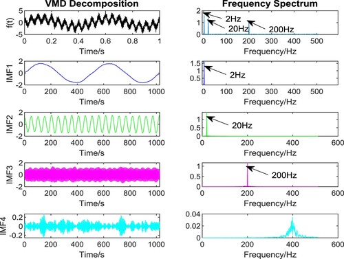
Figure 4. Decomposition result based on SPSO-VMD method.

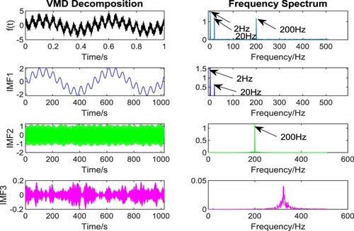
Figure 5. Decomposition result based on GA-VMD method.

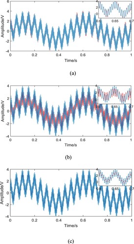
The simulation signal is decomposed into several mode components by the AVMD algorithm. Time–frequency matrix is constructed form the decomposed mode components, and then the time–frequency matrix is decomposed by SVD to obtain the corresponding time–frequency subspaces and singular values. In Figure 6(a), the signal filtered by the AVMD-SVD method retains the spectral characteristics of the simulation signal. While in Figure 6(b), the reconstructed signal based on the SPSO-VMD-SVD method is distorted, and the denoising is invalid. It can be found from Figure 6(c) that the waveform after noise reduction by the GA-VMD-SVD method is also distorted, and the amplitude information of $x\left(t\right)$ is not retained.

Figure 6. Simulation signal denoising results based on different methods. (a) Noise reduction result of simulation signal by AVMD-SVD method (b) Noise reduction result of simulation signal by SPSO-VMD-SVD method (c) Noise reduction result of simulation signal by GA-VMD-SVD method.

4.2. Performance indicators

In this paper, output signal-to-noise ratio ($SN{R}_{out}$), mean square error (MSE), mean absolute error (MAE), and energy loss coefficient (e) (Tang & Wang, 2016) are used to evaluate the denoising effect. The higher the $SN{R}_{out}$, the better the denoising effect. MSE and MAE indicate the closeness of the denoising signal to the pure signal, and lower MSE and MAE indicate that the denoising signal is closer to the pure signal. The AVMD optimization parameter method is carried out with the iterative increase of the number of modes $K$. At the beginning of the calculation, the $K$ value is usually too small. At this time, the reconstructed signal may be very different from the original signal. The smaller the energy loss coefficient, the more the characteristics of the original signal are maintained, and the better the denoising effect. The specific calculation formulas are defined as follows: (18) $\begin{array}{rl}SN{R}_{out}& =10\lg \left(\sum _{i=1}^N{\left(x\left(t\right)\right)}^2/\sum _{i=1}^N{\left(x\left(t\right)-\hat{x}\left(t\right)\right)}^2\right)\end{array}$(18) (19) $\begin{array}{rl}MSE& =\frac{1}{N}\sum _{i=1}^N{\left(x\left(t\right)-\hat{x}\left(t\right)\right)}^2\end{array}$(19) (20) $\begin{array}{rl}MAE& =\frac{1}{N}\sum _{i=1}^N|\left(x\left(t\right)-\hat{x}\left(t\right)\right)|\end{array}$(20) (21) $\begin{array}{rl}e& ={||x\left(t\right)-\hat{x}\left(t\right)|{|}_2^2/||x\left(t\right)||}_2^2\end{array}$(21) where $x\left(t\right)$ is the pure signal, $\hat{x}\left(t\right)$ is the denoising signal, $N$ is the length of the signal.

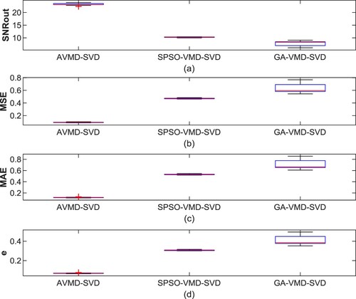
Twenty sets of experiments are carried out with different optimization methods for the simulation signal. Figure 7 shows the results of performance evaluation indicators of different methods for denoising. Compared with denoising methods of SPSO-VMD-SVD and GA-VMD-SVD, the $SN{R}_{out}$ of AVMD-SVD is the highest. The MSE, MAE, and energy loss coefficients of the AVMD-SVD method are all lowest than those of the SPSO-VMD-SVD method and GA-VMD-SVD method, and the fluctuation range is very small.

Figure 7. Denoising performance evaluation of different methods: (a) Box diagram of $SN{R}_{out}$ (b) Box diagram of MSE (c) Box diagram of MAE (d) Box diagram of energy loss coefficient.

4.3. Denoising analysis of pipeline leakage signal

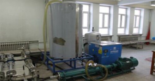
In this paper, the pipeline leakage signal is collected by the natural gas pipeline leak detection simulation experiment platform of Northeast Petroleum University, seeing in Figure 8. The length of the simulated pipeline on the experimental platform is 160m, a pipe diameter of DN50, and a pipe wall thickness of 1 centimetre. In order to simulate a pipeline leakage in the field, the pipeline has a total of 15 leak points, and every two adjacent leak points are separated by 10 metres. The experimental software uses LABVIEW to compile the upper computer, and the data acquisition uses the NI-9215 acquisition board of NI Corporation. The sampling frequency is 3 KHz. Upload the collected data to the computer.

Figure 8. Pipeline leak detection simulation experiment platform.

For the pipeline leakage signal, three methods are used to optimize the parameter pair of the VMD for five times. The specific results of optimizing the parameters of VMD are shown in Table 3. The variance of the parameters optimized by the AVMD method is the smallest, the fluctuation is small, and it has strong robustness. The parameter pair $\left[K,\alpha \right]$ optimized by the AVMD method has the smallest variance, small fluctuation, and strong robustness. The SPSO-VMD method optimizes the variance of the $\alpha$ value and its fluctuation range is large. The variances of $K$ value and $\alpha$ value obtained by GA-VMD method optimization are large, and the robustness of this method is poor. The average values of the VMD parameter pairs optimized by the three methods are used as the initial value parameters of VMD, and the collected pipeline leakage signal is decomposed. Figure 9 is the decomposition effect of the pipeline leakage signal. The sampling frequency of the pipeline leakage signal is 3 kHz. The number of sampling points is 8192. The pipeline leakage signal is decomposed into 3 effective mode components and 7 noise components with centre frequencies of 12, 30, and 131 Hz by the AVMD method. While the SPSO-VMD method can only decompose 1 effective IMF and 1 noise component, the GA-VMD method also decomposes 1 effective IMF and 1 noise component. From the above analysis, it can be concluded that compared with SPSO-VMD and GA-VMD optimization methods, the AVMD method can separate the effective components and the noise components of the signal completely. It shows that AVMD proposed in this paper has better feasibility and superiority. Table 4 shows the results of four performance evaluation indexes after denoising the pipeline leakage signal. The performance evaluation index results of the signal filtering method of the AVMD method are expressed in bold. Through comparison, it is found that the $SN{R}_{out}$ is the highest of AVMD-SVD method, and MSE, MAE, and energy loss coefficient are the lowest of AVMD-SVD method. The AVMD-SVD method has obvious advantages for the denoising of pipeline leakage signal.

Figure 9. Decomposition results of different methods. (a) Decomposition effect of the pipeline leakage signal by the AVMD method (b) Decomposition effect of the pipeline leakage signal by the SPSO-VMD method (c) Decomposition effect of the pipeline leakage signal by the GA-VMD method.

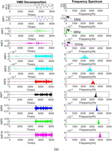
Table 3. Optimization results of pipeline leakage signal.

	AVMD		SPSO-VMD		GA-VMD
Sequence number	$K$	$\alpha$	$K$	$\alpha$	$K$	$\alpha$
1	10	950	2	2240	2	863
2	10	950	2	3110	9	4110
3	10	950	2	3958	2	748
4	10	900	2	3907	2	702
5	10	950	2	3120	2	386
Mean value	10	940	2	2400	3	1362
Variance	0	0.5e+03	0	4.9e+05	9.8	2.4e+06

Table 4. Denoising performance evaluation index of different methods.

Methods	$SN{R}_{out}$	MSE	MAE	Energy loss coefficient
AVMD-SVD	26.1036	0.0025	0.0049	0.0495
SPSO-VMD-SVDD	25.6950	0.0028	0.0051	0.0518
GA-VMD-SVD	25.8980	0.0027	0.0050	0.0506

5. Conclusion

In this paper, a signal denoising method based on the AVMD and SVD has been proposed in order to denoise the leakage signal of pipelines. The control parameters $\left[K,\alpha \right]$ of VMD have been optimized by AVMD. A new adaptive method for selecting VMD parameters has been established by adopting the fitness function based on RCMDE. Compared with other optimization algorithms, it has been shown that the parameters optimized by the AVMD method could make the VMD decomposition obtain more effective mode components, and avoid under-decomposition or over-decomposition. The AVMD-SVD method has been used to filter noisy signals, and it has been applied to natural gas pipeline leakage signal. The experiment has been demonstrated that this method could effectively filter out noise, and retain the original characteristics for leakage signal of pipeline.

Disclosure statement

No potential conflict of interest was reported by the author(s).

Additional information

Funding

This work was supported in part by the National Natural Science Foundation of China [grants numbers 61873058 and NSFC 51575407], China Petroleum Science and Technology Innovation Fund [grant number 2018D-5007-0302], The Natural Science Foundation of Heilongjiang Province [grant number LH2020F005], Youth Science Foundation Project of Northeast Petroleum University [grant number 2018QNL-33], The Project Supported by The Open Fund of The Key Laboratory for Metallurgical Equipment and Control of Ministry of Education in Wuhan University of Science and Technology [grant number MECOF2019B01].

References

- Azami, H., Rostaghi, M., Abásolo, D., & Escudero, J. (2017). Refined composite multiscale dispersion entropy and its application to biomedical signals. IEEE Transactions on Biomedical Engineering, 64(12), 2872–2879. https://doi.org/https://doi.org/10.1109/TBME.2017.2679136
- Dragomiretskiy, K., & Zosso, D. (2014). Variational mode decomposition. IEEE Transactions on Signal Processing, 62(3), 531–544. https://doi.org/https://doi.org/10.1109/TSP.2013.2288675
- Gao, H., Ma, L., Dong, H., Lu, J., & Li, G. (2020). An improved two-dimensional variational mode decomposition algorithm and its application in oil pipeline image. Systems Science & Control Engineering, 8(1), 297–307. https://doi.org/https://doi.org/10.1080/21642583.2020.1756523
- Gu, R., Chen, J., Hong, R., Wang, H., & Wu, W. (2020). Incipient fault diagnosis of rolling bearings based on adaptive variational mode decomposition and teager energy operator. Measurement, 149(2), 106941. https://doi.org/https://doi.org/10.1016/j.measurement.2019.106941
- Huang, H. B., Huang, X. R., Yang, M. L., Lim, T. C., & Ding, W. P. (2018). Identification of vehicle interior noise sources based on wavelet transform and partial coherence analysis. Mechanical Systems and Signal Processing, 109, 247–267. https://doi.org/https://doi.org/10.1016/j.ymssp.2018.02.045
- Huang, N. E., Shen, Z., Long, S. R., Wu, M. C., Shih, H. H., Zheng, Q., … Liu, H. H. (1998). The empirical mode decomposition and the Hilbert spectrum for nonlinear and non-stationary time series analysis. Proceedings of the Royal Society of London. Series A: Mathematical, Physical and Engineering Sciences, 454(1971), 903–995. https://doi.org/https://doi.org/10.1098/rspa.1998.0193
- Lahmiri, S., & Boukadoum, M. (2015). A weighted bio-signal denoising approach using empirical mode decomposition. Biomedical Engineering Letters, 5(2), 131–139. https://doi.org/https://doi.org/10.1007/s13534-015-0182-2
- Li, H., Liu, T., Wu, X., & Chen, Q. (2019). Research on bearing fault feature extraction based on singular value decomposition and optimized frequency band entropy. Mechanical Systems and Signal Processing, 118, 477–502. https://doi.org/https://doi.org/10.1016/j.ymssp.2018.08.056
- Li, H., Liu, T., Wu, X., & Chen, Q. (2020). An optimized VMD method and its applications in bearing fault diagnosis. Measurement, 166(4), 108185. https://doi.org/https://doi.org/10.1016/j.measurement.2020.108185
- Li, J., Zheng, Q., Qian, Z., & Yang, X. (2019). A novel location algorithm for pipeline leakage based on the attenuation of negative pressure wave. Process Safety and Environmental Protection, 123, 309–316. https://doi.org/https://doi.org/10.1016/j.psep.2019.01.010
- Liang, W., Zhang, L., Xu, Q., & Yan, C. (2013). Gas pipeline leakage detection based on acoustic technology. Engineering Failure Analysis, 31, 1–7. https://doi.org/https://doi.org/10.1016/j.engfailanal.2012.10.020
- Liu, C., Li, Y., Fang, L., & Xu, M. (2017). Experimental study on a de-noising system for gas and oil pipelines based on an acoustic leak detection and location method. International Journal of Pressure Vessels and Piping, 151, 20–34. https://doi.org/https://doi.org/10.1016/j.ijpvp.2017.02.001
- Liu, C., Li, Y., Yan, Y., Fu, J., & Zhang, Y. (2015). A new leak location method based on leakage acoustic waves for oil and gas pipelines. Journal of Loss Prevention in the Process Industries, 35, 236–246. https://doi.org/https://doi.org/10.1016/j.jlp.2015.05.006
- Lu, J., Yue, J., Zhu, L., & Li, G. (2020). Variational mode decomposition denoising combined with improved Bhattacharyya distance. Measurement, 151(1), 107283. https://doi.org/https://doi.org/10.1016/j.measurement.2019.107283
- Muggleton, J. M., Hunt, R., Rustighi, E., Lees, G., & Pearce, A. (2020). Gas pipeline leak noise measurements using optical fibre distributed acoustic sensing. Journal of Natural Gas Science and Engineering, 78(1), 103293. https://doi.org/https://doi.org/10.1016/j.jngse.2020.103293
- Murvay, P. S., & Silea, I. (2012). A survey on gas leak detection and localization techniques. Journal of Loss Prevention in the Process Industries, 25(6), 966–973. https://doi.org/https://doi.org/10.1016/j.jlp.2012.05.010
- Rostaghi, M. (2016). Dispersion entropy: A measure for time-series analysis. IEEE Signal Processing Letters, 23(5), 610–614. https://doi.org/https://doi.org/10.1109/LSP.2016.2542881
- Tang, G. J., & Wang, X. L. (2016). An incipient fault diagnosis method for rolling bearing based on improved variational mode decomposition and singular value difference spectrum. Journal of Vibration, Measurement and Diagnosis, 36(4), 700–707. https://doi.org/https://doi.org/10.16450/j.cnki.issn.1004-6801.2016.04.014
- Wang, S. Q., Lin, Y. Y., Meng, Y. D., & Gao, Z. Q. (2012). Model order determination based on singular value decomposition. Zhendong yu Chongji (Journal of Vibration and Shock), 31(15), 87–91.
- Xiao, R., Hu, Q., & Li, J. (2019). Leak detection of gas pipelines using acoustic signals based on wavelet transform and support vector machine. Measurement, 146, 479–489. https://doi.org/https://doi.org/10.1016/j.Measurement.2019.06.050
- Xin, L., Liu, Z., Dou, J., Yang, Z., Zhang, X., & Liu, Z. (2020). A robust white-light interference signal leakage sampling correction method based on wavelet transform. Optics and Lasers in Engineering, 133(1), 106156. https://doi.org/https://doi.org/10.1016/j.optlaseng.2020.106156
- Yang, K., Wang, G., Dong, Y., Zhang, Q., & Sang, L. (2019). Early chatter identification based on an optimized variational mode decomposition. Mechanical Systems and Signal Processing, 115, 238–254. https://doi.org/https://doi.org/10.1016/j.ymssp.2018.05.052
- Yi, C., Lv, Y., & Dang, Z. (2016). A fault diagnosis scheme for rolling bearing based on particle swarm optimization in variational mode decomposition. Shock and Vibration, 2016. Article ID 9372691. https://doi.org/https://doi.org/10.1155/2016/9372691
- Zhang, Y., Chen, S., Li, J., & Jin, S. (2014). Leak detection monitoring system of long distance oil pipeline based on dynamic pressure transmitter. Measurement, 49, 382–389. https://doi.org/https://doi.org/10.1016/j.measurement.2013.12.009
- Zhang, X., Miao, Q., Zhang, H., & Wang, L. (2018). A parameter-adaptive VMD method based on grasshopper optimization algorithm to analyze vibration signals from rotating machinery. Mechanical Systems and Signal Processing, 108, 58–72. https://doi.org/https://doi.org/10.1016/j.ymssp.2017.11.029
- Zhang, X., Peng, J., Xu, M., Yang, W., Zhang, Z., Guo, H., & Feng, Y. (2017). Denoise diffusion-weighted images using higher-order singular value decomposition. Neuroimage, 156, 128–145. https://doi.org/https://doi.org/10.1016/j.neuroimage.2017.04.017
- Zhao, M., & Jia, X. (2017). A novel strategy for signal denoising using reweighted SVD and its applications to weak fault feature enhancement of rotating machinery. Mechanical Systems and Signal Processing, 94, 129–147. https://doi.org/https://doi.org/10.1016/j.ymssp.2017.02.036
- Zhou, Y., Zhang, Y., Yang, D., Lu, J., Dong, H., & Li, G. (2020). Pipeline signal feature extraction with improved VMD and multi-feature fusion. Systems Science & Control Engineering, 8(1), 318–327. https://doi.org/https://doi.org/10.1080/21642583.2020.1765218
- Zhou, Y., & Zhu, Z. (2019). A hybrid method for noise suppression using variational mode decomposition and singular spectrum analysis. Journal of Applied Geophysics, 161, 105–115. https://doi.org/https://doi.org/10.1016/j.jappgeo.2018.10.025