Distributed filtering for delayed nonlinear system with random sensor saturation: a dynamic event-triggered approach

Abstract

This paper is concerned with the distributed filtering problem for a class of delayed nonlinear systems with random sensor saturation (RSS) under a dynamic event-triggered mechanism. The nonlinear function is assumed to satisfy the Lipschitz condition. A dynamic event-triggered mechanism is employed to further reduce the innovation transmission frequencies among the adjacent nodes. Both the Bernoulli distributed random variables and saturation function are employed to model the phenomenon of RSS. The aim of this paper is to design a sub-optimal filter such that the covariance of the filtering error has an upper bound, which is minimized by appropriately computing the filter gain. Furthermore, the error boundedness is analysed and a sufficient criterion is presented to ensure that the filtering error is mean-square bounded. Finally, a numerical example is provided to verify the effectiveness of the proposed filtering algorithm.

Keywords:

• Nonlinear delayed system
• dynamic event-triggered mechanism
• distributed filtering
• RSS

1. Introduction

Wireless sensor network (WSN) can connect a large number of intelligent sensors to work together via the communication networks with limited bandwidth. Compared with the traditional point-to-point sensor system, the WSN has the advantages of scalability, flexibility, low cost and easy installation (Shi et al., 2014), which has been widely used in intelligent transportation (Tacconi et al., 2010; Yousef et al., 2010), process control (Gungor & Hancke, 2009; Sun & El-Farra, 2012), intelligent household, intelligent medical (Hu et al., 2013) and other fields (Ciuonzo et al., 2013; Ciuonzo & Salvo Rossi, 2017). Accordingly, the filtering problem based on WSN has attracted a great deal of attention. To mention a few, the distributed filtering problem has been investigated in Wen et al. (2018) for discrete-time state-saturated systems with random nonlinearity and measurement loss, where the topological structure of sensor network (SN) has been described by a digraph. In Liu et al. (2019), the distributed filtering problem has been handled for a class of continuous-time stochastic systems over SN with Markovian switching topology, and the considered time-varying topology may stochastically changes among a set of disconnected graphs at every sampling instant. To reduce the communication load, in Shen et al. (2020), the distributed recursive filtering scheme has been designed for stochastic discrete systems subject to Round-Robin protocol, and the matrix simplification technique has been used to tackle the problem of topological sparseness of SN. For 2-D systems with measurement degradations over SN, in Wang et al. (2020), the recursive filter has been designed and an upper bound of the error covariance has been constructed by exploiting the stochastic analysis and the mathematical induction approach.

The network-induced phenomena, which are mainly caused by the network characteristics, could worsen the filtering method performance if not handled properly (Walsh & Ye, 2001; Zhang et al., 2001; Hu et al., 2016). At present, the sensor saturation problem has attracted great interest of researchers (Ding et al., 2013; Li et al., 2020; Singh, 2007). Motivated by the widespread sensor saturation problem, in Hu et al. (2012), a probability-guaranteed $H_{\mathrm{\infty }}$ finite-horizon filtering algorithm has been given, where the saturation function has been decomposed into a linear part and a sector-bounded nonlinear part. In fact, the sensor saturation may be affected by some uncertain factors, in consequence, it is more practical to investigate the random sensor saturation (RSS) for large-scale SN. In Wang et al. (2012), a novel sensor measurement model has been established to account for the RSS by using a set of Bernoulli distributed white sequences with known conditional probabilities. In consideration of both variance-constrained and $H_{\mathrm{\infty }}$ performance, the multi-objective filter has been put forward in Li et al. (2020) for multi-rate time-varying systems with RSS.

It is well recognized that the state delays exist in many real-word systems. Thus, many results have been developed to tackle the delays and avoid the great deterioration of system performance (Chen et al., 2019; Chen & Xu, 2014). For example, in (Du et al., 2016), an optimal filtering algorithm has been developed for a class of networked stochastic systems, where both the state delay and missing measurements have been taken into account. On the other hand, the extended Kalman-type recursive filter has been designed in Mao et al. (2019) for a class of nonlinear stochastic systems subject to missing measurement, fixed time-delay and uniform quantization, where the Round-Robin protocol has been employed to regulate the transmissions and lighten the network transmission burden. In Mao et al. (2017), the recursive filtering algorithm has been designed for a class of delayed nonlinear systems with event-based communication protocols, and a time-varying triggered threshold has been introduced to dynamically regulate the networked communications. In particular, the event-triggering mechanism is a sporadic transmission strategy if the current signal meets a prescribed event generator condition. In order to reduce network load, Arzen (1999) proposed event-triggering mechanism and designed a PID controller. Recently, in order to further save network resources, a dynamic event-triggered mechanism has been put forward in Girard (2015) by introducing dynamic auxiliary variables. Subsequently, the comparisons between static and dynamic event-triggered mechanism have been specified in Ge et al. (2019), where the event-triggered weighted matrix has been obtained by a recursive convex optimization algorithm and a distributed set-membership estimator has been designed. Based on the time-varying topology, the recursive distributed filtering problem has been investigated in Li et al. (2020) for nonlinear time-varying systems under a dynamic event-triggered mechanism. Unfortunately, to the best of the authors' knowledge, the recursive filter design problem has not been thoroughly addressed yet for nonlinear delayed systems with dynamic event-triggering mechanism and RSS. Besides, the boundedness analysis is desirable on handling the issue of corresponding distributed filtering.

Motivated by the above analysis, we aim to address the distributed filter design problem for a class of delayed nonlinear systems with RSS under dynamic event-triggered mechanism. Here, the time-invariant delay is considered. The RSS is modelled by the Bernoulli distributed random variable and a saturation function. Moreover, an auxiliary variable that is correlated with innovation is used to construct the dynamic event-triggered mechanism. The contributions of this paper can be highlighted as follows: (i) the proposed time-varying system is fairly comprehensive that covers time delay, delay-dependent nonlinearity and RSS, thereby better reflecting the engineering reality; (ii) the recursive distributed filtering scheme is developed for the delayed system under the dynamic event-triggered communication mechanism; and (iii) a novel sufficient criterion is given to guarantee a bounded variance of filtering errors in the mean square sense.

Notations The notations used throughout this paper are standard. ${\mathbb{R}}^n$ denotes the n-dimensional Euclidean space. $\parallel \cdot \parallel$ is the Euclidean norm of real vectors or the spectral norm of real matrices. For a matrix P, $P^T$ and $P^{-1}$ represent its transpose and inverse, respectively. $\mathbb{E}\left\{x\right\}$ denotes the mathematical expectation of the random variable x. I stands for the identity matrix with appropriate dimension. $\mathrm{t}\mathrm{r}\left\{P\right\}$ represents the trace of matrix P. $\mathrm{d}\mathrm{i}\mathrm{a}\mathrm{g}\{P_1,P_2,\dots ,P_N\}$ represents a block-diagonal matrix with matrices $P_1,P_2,\dots ,P_N$ on the diagonal. Matrices, if their dimensions are not explicitly stated, are assumed to be compatible for algebraic operations.

2. Problem formulation and preliminaries

In this paper, we use a digraph $\mathcal{G}=(\mathcal{V},\mathcal{E},\mathcal{A})$ to describe the communication topology of the considered sensor network. The digraph $\mathcal{G}$ contains a vertex set $\mathcal{V}=\{v_1,v_2,\dots ,v_N\}$, an edge set $\mathcal{E}\subseteq \mathcal{V}\times \mathcal{V}$, and an adjacency matrix $\mathcal{A}=[a_{ij}{]}_{N\times N}$ with nonnegative elements, where N is the number of sensor nodes. Moreover, we assume that $a_{ii}=1$ for all $i\in \mathcal{V}$. The set of neighbours of node $i\in \mathcal{V}$ plus the node itself is denoted by ${\mathcal{N}}_i=\{j\in \mathcal{V}|(i,j)\in \mathcal{E}\}$.

Consider the following discrete time-varying systems with RSS: (1) $\begin{array}{rl}{\overrightarrow{x}}_{k+1}& ={\overrightarrow{A}}_k{\overrightarrow{x}}_k+{\overrightarrow{B}}_{k-\tau }{\overrightarrow{x}}_{k-\tau }+\overrightarrow{f}({\overrightarrow{x}}_k,{\overrightarrow{x}}_{k-\tau })+{\overrightarrow{D}}_k{\overrightarrow{\omega }}_k\end{array}$(1) (2) $\begin{array}{rl}{y}_{i,k}& =(1-{\alpha }_{i,k})\sigma \left(C_{i,k}{\overrightarrow{x}}_k\right)+{\alpha }_{i,k}{C}_{i,k}{\overrightarrow{x}}_k+{\nu }_{i,k}\end{array}$(2) where k is the sampling instant, ${\overrightarrow{x}}_k\in {\mathbb{R}}^n$ represents the state vector to be estimated, the initial state is ${\overrightarrow{x}}_m={\overrightarrow{\phi }}_m$ $(m=-\tau ,-\tau +1,\dots ,0)$, $y_{i,k}\in {\mathbb{R}}^q$ denotes the measurement output of ith sensor, ${\overrightarrow{A}}_k$, ${\overrightarrow{B}}_{k-\tau }$, ${\overrightarrow{D}}_k$, and $C_{i,k}$ are known matrices with appropriate dimensions. ${\overrightarrow{\omega }}_k\in {\mathbb{R}}^p$ and ${\nu }_{i,k}\in {\mathbb{R}}^q$ are zero mean additive noises with covariances ${\overrightarrow{Q}}_k>0$ and $R_{i,k}>0$, respectively. The random variable ${\alpha }_{i,k}$ $(i=1,\dots ,N)$, which describes the phenomenon of RSS, takes value on 0 or 1 with (3) $\mathrm{P}\mathrm{r}\mathrm{o}\mathrm{b}\{{\alpha }_{i,k}=1\}={\overline{\alpha }}_i,\mathrm{P}\mathrm{r}\mathrm{o}\mathrm{b}\{{\alpha }_{i,k}=0\}=1-{\overline{\alpha }}_i$(3) where ${\overline{\alpha }}_i\in [0,1]$ $(i=1,\dots ,N)$ is a known constant. It is assumed that ${\alpha }_{i,k}$, ${\overrightarrow{\omega }}_k$ and ${\nu }_{i,k}$ are mutually independent. The saturation function $\sigma (\cdot )$ is defined as $\sigma \left(s\right)\triangleq \left[{\sigma }_1\right(s_1\left){\sigma }_2\right(s_2)\dots {\sigma }_q(s_q){]}^T$where (4) ${\sigma }_i\left(s_i\right)=\mathrm{s}\mathrm{i}\mathrm{g}\mathrm{n}\left(s_i\right)\mathrm{m}\mathrm{i}\mathrm{n}\{s_{i,\mathrm{m}\mathrm{a}\mathrm{x}},|s_i|\}$(4) and $s_{i,\mathrm{m}\mathrm{a}\mathrm{x}}$ is the ith element of the saturation level vector $s_{\mathrm{m}\mathrm{a}\mathrm{x}}$.

Assumption 2.1

The nonlinear vector function $\overrightarrow{f}(\cdot ,\cdot )\in {\mathbb{R}}^n$ satisfies $f(0,0)=0$ and the following bounded condition: (5) $\begin{array}{rl}& \parallel \overrightarrow{f}(x_1,y_1)-\overrightarrow{f}(x_2,y_2)\parallel \\ & \le \parallel {\overrightarrow{S}}_1(x_1-x_2)\parallel +\parallel {\overrightarrow{S}}_2(y_1-y_2)\parallel \end{array}$(5) with ${\overrightarrow{S}}_1$ and ${\overrightarrow{S}}_2$ are known real constant matrices.

In this paper, the dynamic event-triggered communication protocol is adopted to reduce the network transmission burden. Before presenting a specific event generator function, let us explain some relevant variables. ${\hat{x}}_{i,k|k-1}$ $(i=1,2,\dots ,N)$ denotes the one-step prediction at instant k−1 of node i, and the corresponding innovation ${\tilde{y}}_{i,k}$ can be written as (6) ${\tilde{y}}_{i,k}=y_{i,k}-(1-{\overline{\alpha }}_i)\sigma \left(C_{i,k}{\hat{x}}_{i,k|k-1}\right)-{\overline{\alpha }}_i{C}_{i,k}{\hat{x}}_{i,k|k-1}.$(6) Let $b_{i,t}$ represent the last triggering time corresponding to the instant k, and therefore ${\tilde{y}}_{i,b_{i,t}}$ is the innovation at $b_{i,t}$. Next, the dynamic event generator function is proposed as follows: (7) $\psi ({\theta }_i,r_{i,k},{\sigma }_i,{\eta }_{i,k})={\theta }_i(\parallel r_{i,k}\parallel -{\sigma }_i)-{\eta }_{i,k}$(7) where $r_{i,k}={\tilde{y}}_{i,k}-{\tilde{y}}_{i,b_{i,t}}$, ${\sigma }_i$ and ${\theta }_i$ are given positive scalars. The auxiliary offset variable ${\eta }_{i,k}\in \mathbb{R}$ in (7(7) $\psi ({\theta }_i,r_{i,k},{\sigma }_i,{\eta }_{i,k})={\theta }_i(\parallel r_{i,k}\parallel -{\sigma }_i)-{\eta }_{i,k}$(7) ) satisfies the following equation: (8) ${\eta }_{i,k+1}={\lambda }_i{\eta }_{i,k}+{\sigma }_i-\parallel r_{i,k}\parallel ,{\eta }_{0,i}={\overline{\eta }}_{0,i}$(8) where the initial state ${\overline{\eta }}_{0,i}\ge 0$ is a known constant. In (7(7) $\psi ({\theta }_i,r_{i,k},{\sigma }_i,{\eta }_{i,k})={\theta }_i(\parallel r_{i,k}\parallel -{\sigma }_i)-{\eta }_{i,k}$(7) ) and (8(8) ${\eta }_{i,k+1}={\lambda }_i{\eta }_{i,k}+{\sigma }_i-\parallel r_{i,k}\parallel ,{\eta }_{0,i}={\overline{\eta }}_{0,i}$(8) ), ${\theta }_i$ and ${\lambda }_i$ are prescribed positive scalars satisfying (9) $0<{\lambda }_i<1,{\theta }_i{\lambda }_i\ge 1.$(9) The innovation of the ith node will be transmitted to the corresponding nodes to update the innovation recorded by its zero-order holder, if and only if, the function $\psi (\cdot ,\cdot ,\cdot ,\cdot )\ge 0$. Therefore, we define the triggered instant sequence of node i by $0=b_{i,0}<b_{i,1}<\cdots <b_{i,t}<\cdots$, which is determined iteratively by (10) $b_{i,t+1}=\mathrm{i}\mathrm{n}\mathrm{f}\{k|k>b_{i,t},\psi ({\theta }_i,r_{i,k},{\sigma }_i,{\eta }_{i,k})\ge 0\}.$(10) Then, the signal used to update the local estimation can be written as follows: (11) ${\overline{\tilde{y}}}_{i,k}={\tilde{y}}_{i,b_{i,t}},k\in \{b_{i,t},b_{i,t}+1,\dots ,b_{i,t+1}-1\}.$(11)

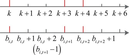
Remark 2.1

Now, we explain the differences between k and $b_{i,t}$ in order to make the event-triggered mechanism to be understood easily. For example, it can be seen from Figure 1 that k represents the sampling instant of the sensor nodes, while k, k + 3 and k + 4 are the triggered instants of the ith node, respectively. Accordingly, $b_{i,t}$ emphasizes the sense of nearest triggered instant and $b_{i,t+1}$ is the next triggered instant.

Figure 1. Triggered instants.

Lemma 2.1

Ge et al., 2019

For prescribed positive scalars ${\lambda }_i$ and ${\theta }_i$ satisfying (9(9) $0<{\lambda }_i<1,{\theta }_i{\lambda }_i\ge 1.$(9) ), the auxiliary offset variable (12) ${\eta }_{i,k}\ge 0$(12) holds for all $k\in \mathbb{N}$.

Remark 2.2

Note that the dynamic event-triggered mechanism can dynamically adjust the communication frequency. Compared to the static event-triggered function $z(r_{i,k},{\sigma }_i)=\parallel r_{i,k}-{\sigma }_i\parallel$, the auxiliary variable ${\eta }_{i,k}$ in (7(7) $\psi ({\theta }_i,r_{i,k},{\sigma }_i,{\eta }_{i,k})={\theta }_i(\parallel r_{i,k}\parallel -{\sigma }_i)-{\eta }_{i,k}$(7) ) described by (8(8) ${\eta }_{i,k+1}={\lambda }_i{\eta }_{i,k}+{\sigma }_i-\parallel r_{i,k}\parallel ,{\eta }_{0,i}={\overline{\eta }}_{0,i}$(8) ) can be seen as the estimation of $z(r_{i,k},{\sigma }_i)$. ${\theta }_i$ is a parameter that is used to adjust the trigger frequency. The dynamic event-triggered mechanism can further reduce the consumption of communication resources. It is easy to see that the impact of ${\eta }_{i,k}$ to $\psi ({\theta }_i,r_{i,k},{\sigma }_i,{\eta }_{i,k})$ is negligible when ${\theta }_i\to +\mathrm{\infty }$. Consequently, the dynamic event-triggered function degenerates into the static event-triggered function. On the other hand, the threshold ${\sigma }_i$ of static event-triggered mechanism is time-invariant. By introducing an offset variable generated through the auxiliary systems, the threshold of dynamic event-triggered mechanism is varying and the interval $b_{i,t+1}-b_{i,t}$ is dynamically adjusted.

For systems (1(1) $\begin{array}{rl}{\overrightarrow{x}}_{k+1}& ={\overrightarrow{A}}_k{\overrightarrow{x}}_k+{\overrightarrow{B}}_{k-\tau }{\overrightarrow{x}}_{k-\tau }+\overrightarrow{f}({\overrightarrow{x}}_k,{\overrightarrow{x}}_{k-\tau })+{\overrightarrow{D}}_k{\overrightarrow{\omega }}_k\end{array}$(1) )–(2(2) $\begin{array}{rl}{y}_{i,k}& =(1-{\alpha }_{i,k})\sigma \left(C_{i,k}{\overrightarrow{x}}_k\right)+{\alpha }_{i,k}{C}_{i,k}{\overrightarrow{x}}_k+{\nu }_{i,k}\end{array}$(2) ), the recursive filters to be designed are of the following forms: (13) $\begin{array}{rl}{\hat{x}}_{i,k+1|k}& ={\overrightarrow{A}}_k{\hat{x}}_{i,k|k}+{\overrightarrow{B}}_{k-\tau }{\hat{x}}_{i,k-\tau |k-\tau }\\ & +\overrightarrow{f}({\hat{x}}_{i,k|k},{\hat{x}}_{i,k-\tau |k-\tau }),\end{array}$(13) (14) $\begin{array}{rl}{\hat{x}}_{i,k+1|k+1}& ={\hat{x}}_{i,k+1|k}+\sum _{j\in {\mathcal{N}}_i}{a}_{ij}{K}_{ij,k+1}{\overline{\tilde{y}}}_{j,k+1}\end{array}$(14) where $K_{ij,k+1}$ are the filter parameters to be designed.

Remark 2.3

Compared with the existing results (e.g. Mao et al. (2019), Mao et al. (2017) and Li et al. (2020)), the recursive filtering algorithm to be given has the following features: (i) a new distributed filtering scheme is given for nonlinear delayed systems with RSS and dynamic event-triggered mechanism in a unified framework; (ii) the nonlinear disturbance influenced by both current and delayed information is common in engineering case and the related influences are considered when designing the filter; and (iii) the available information of time delay and dynamic event-triggered mechanism is employed in the filter with hope to compensate the corresponding impacts. Viewed from another perspective, compared to linear matrix inequality method, the advantages of recursive method lie in its potential in the online applications.

Remark 2.4

The problem of the distributed filtering for discrete time-varying delayed system with dynamic event-triggered mechanism in sensor network has very important practical significance in the target tracking field over the underwater sensor networks (USNs). Firstly, in Yu and Choi (2014), a distributed filtering scheme has been given based on sensor network transmission, which can overcome the defects of underwater centralized fusion target tracking algorithm. Secondly, the working conditions and environments of the sensor node are not ideal, and the changes of temperature, salinity, depth and pressure of sea would inevitably cause time delay. Therefore, the study of filtering problem of delayed systems is more suitable from the practical engineering viewpoint. Finally, the sensor nodes in USNs use batteries to provide the energy. Special underwater environment makes it is hard to replace the depleted batteries, that is, the service life of USNs often depends on the life span of the sensor nodes. In Sun et al. (2018), an event-triggered mechanism that adaptively adjusts the sampling interval has been put forward for target tracking over USNs. Overall, the concerned distributed filtering problem has important significance from the engineering background.

Lemma 2.2

Wen et al., 2018

For $\mathrm{\forall }x,y\in \mathbb{R}$, there exists a real number ${\text{β}}_i\in [0,1]$ such that ${\sigma }_i\left(x\right)-{\sigma }_i\left(y\right)={\text{β}}_i(x-y)$where the saturation function ${\sigma }_i(\cdot )$ $(i=1,2,\dots ,q)$ isdefined in (4(4) ${\sigma }_i\left(s_i\right)=\mathrm{s}\mathrm{i}\mathrm{g}\mathrm{n}\left(s_i\right)\mathrm{m}\mathrm{i}\mathrm{n}\{s_{i,\mathrm{m}\mathrm{a}\mathrm{x}},|s_i|\}$(4) ).

Lemma 2.3

Wen et al., 2018

Let $A=[a_{ij}{]}_{p\times p}$ be a real-valued matrix and $B=\mathrm{d}\mathrm{i}\mathrm{a}\mathrm{g}\{b_1,b_2,\dots ,b_p\}$ be a diagonal random matrix. Then, one has $\mathbb{E}\left\{BA{B}^T\right\}=\mathbb{E}\{B\ast B\}\circ A$where ° is the Hadamard product and $\mathbb{E}\{B\ast B\}$ is defined as $\begin{array}{r}\mathbb{E}\{B\ast B\}=\left[\begin{array}{cccc}\mathbb{E}\left\{b_1^2\right\}& \mathbb{E}\left\{b_1{b}_2\right\}& \dots & \mathbb{E}\left\{b_1{b}_p\right\}\\ \mathbb{E}\left\{b_2{b}_1\right\}& \mathbb{E}\left\{b_2^2\right\}& \dots & \mathbb{E}\left\{b_2{b}_p\right\}\\ ⋮& ⋮& ⋮& ⋮\\ \mathbb{E}\left\{b_p{b}_1\right\}& \mathbb{E}\left\{b_p{b}_2\right\}& \dots & \mathbb{E}\left\{b_p^2\right\}\end{array}\right].\end{array}$

Lemma 2.4

Xie et al., 1994

For any given vectors $X,Y\in {\mathbb{R}}^n$ and a positive scalar $ϵ>0$, the following inequality holds: $X{Y}^T+Y{X}^T\le ϵX{X}^T+{ϵ}^{-1}Y{Y}^T.$

The main objective of this paper is to design a set of distributed filters based on local estimation and triggered innovations ${\overline{\tilde{y}}}_{i,k}(i\in {\mathcal{N}}_i)$ such that an upper bound of filtering error covariance is obtained and the desired filter gain is provided to minimize such an upper bound at each time step. Furthermore, a sufficient condition is given to guarantee the mean-square boundedness of the filtering error.

3. Main results

In this section, the forms of one-step prediction error covariance and filtering error covariance are given firstly. Then, the upper bound on the filtering error covariance is calculated by employing the stochastic analysis technique. Moreover, the desired filtering gain is constructed based on the solutions to Riccati-like matrix difference equations. Finally, the boundedness analysis of filtering error is also discussed.

3.1. Design of the filter gain

For node i, let ${\tilde{x}}_{i,k+1|k}={\overrightarrow{x}}_{k+1}-{\hat{x}}_{i,k+1|k}$ be the one-step prediction error and ${\tilde{x}}_{i,k+1|k+1}={\overrightarrow{x}}_{k+1}-{\hat{x}}_{i,k+1|k+1}$ represent the filter error. According to (1(1) $\begin{array}{rl}{\overrightarrow{x}}_{k+1}& ={\overrightarrow{A}}_k{\overrightarrow{x}}_k+{\overrightarrow{B}}_{k-\tau }{\overrightarrow{x}}_{k-\tau }+\overrightarrow{f}({\overrightarrow{x}}_k,{\overrightarrow{x}}_{k-\tau })+{\overrightarrow{D}}_k{\overrightarrow{\omega }}_k\end{array}$(1) ), (2(2) $\begin{array}{rl}{y}_{i,k}& =(1-{\alpha }_{i,k})\sigma \left(C_{i,k}{\overrightarrow{x}}_k\right)+{\alpha }_{i,k}{C}_{i,k}{\overrightarrow{x}}_k+{\nu }_{i,k}\end{array}$(2) ), (13(13) $\begin{array}{rl}{\hat{x}}_{i,k+1|k}& ={\overrightarrow{A}}_k{\hat{x}}_{i,k|k}+{\overrightarrow{B}}_{k-\tau }{\hat{x}}_{i,k-\tau |k-\tau }\\ & +\overrightarrow{f}({\hat{x}}_{i,k|k},{\hat{x}}_{i,k-\tau |k-\tau }),\end{array}$(13) ) and (14(14) $\begin{array}{rl}{\hat{x}}_{i,k+1|k+1}& ={\hat{x}}_{i,k+1|k}+\sum _{j\in {\mathcal{N}}_i}{a}_{ij}{K}_{ij,k+1}{\overline{\tilde{y}}}_{j,k+1}\end{array}$(14) ), one has (15) $\begin{array}{rl}{\tilde{x}}_{i,k+1|k}& ={\overrightarrow{A}}_k{\tilde{x}}_{i,k|k}+{\overrightarrow{B}}_{k-\tau }{\tilde{x}}_{i,k-\tau |k-\tau }\\ & +{\tilde{\overrightarrow{f}}}_k+{\overrightarrow{D}}_k{\overrightarrow{\omega }}_k,\end{array}$(15) (16) $\begin{array}{rl}{\tilde{x}}_{i,k+1|k+1}& ={\tilde{x}}_{i,k+1|k}-\sum _{j\in {\mathcal{N}}_i}{a}_{ij}{K}_{ij,k+1}{\overline{\tilde{y}}}_{j,k+1}\end{array}$(16) where ${\tilde{\overrightarrow{f}}}_k=\overrightarrow{f}({\overrightarrow{x}}_k,{\overrightarrow{x}}_{k-\tau })-\overrightarrow{f}({\hat{x}}_{i,k|k},{\hat{x}}_{i,k-\tau |k-\tau })$. Adding the following zero terms $\begin{array}{rl}& {\overline{\alpha }}_j{C}_{j,k+1}{\overrightarrow{x}}_{k+1}-{\overline{\alpha }}_j{C}_{j,k+1}{\overrightarrow{x}}_{k+1},\\ & (1-{\overline{\alpha }}_j)\sigma \left(C_{j,k+1}{\overrightarrow{x}}_{k+1}\right)-(1-{\overline{\alpha }}_j)\sigma \left(C_{j,k+1}{\overrightarrow{x}}_{k+1}\right)\end{array}$ into the right-hand side of (16(16) $\begin{array}{rl}{\tilde{x}}_{i,k+1|k+1}& ={\tilde{x}}_{i,k+1|k}-\sum _{j\in {\mathcal{N}}_i}{a}_{ij}{K}_{ij,k+1}{\overline{\tilde{y}}}_{j,k+1}\end{array}$(16) ) and employing Lemma 2.2, we have (17) $\begin{array}{rl}{\tilde{x}}_{i,k+1|k+1}& ={\tilde{x}}_{i,k+1|k}-\sum _{j\in {\mathcal{N}}_i}{a}_{ij}{K}_{ij,k+1}\left\{(1-{\overline{\alpha }}_j){\text{β}}^{\left(j\right)}\right.\\ & \times C_{j,k+1}{\tilde{x}}_{j,k+1|k}+({\overline{\alpha }}_j-{\alpha }_{j,k+1})\sigma (C_{j,k+1}\\ & \times {\overrightarrow{x}}_{k+1})+{\overline{\alpha }}_j{C}_{j,k+1}{\tilde{x}}_{j,k+1|k}+({\alpha }_{j,k+1}-{\overline{\alpha }}_j)\\ & \left.\times C_{j,k+1}{\overrightarrow{x}}_{k+1}+{\nu }_{j,k+1}-r_{j,k+1}\right\}\end{array}$(17) where ${\text{β}}^{\left(j\right)}=\mathrm{d}\mathrm{i}\mathrm{a}\mathrm{g}\{{\text{β}}_1^{\left(j\right)},{\text{β}}_2^{\left(j\right)},\dots ,{\text{β}}_n^{\left(j\right)}\}$, ${\text{β}}_s^{\left(j\right)}(s=1,2,\dots ,n)\in [0,1]$.

For notational simplicity, we set (18) $\begin{array}{rl}& {\tilde{x}}_{k+1|k}\triangleq {\mathrm{c}\mathrm{o}\mathrm{l}}_N\left\{{\tilde{x}}_{i,k+1|k}\right\},x_k\triangleq {\mathrm{c}\mathrm{o}\mathrm{l}}_N\left\{{\overrightarrow{x}}_k\right\},\\ & {\tilde{x}}_{k+1|k+1}\triangleq {\mathrm{c}\mathrm{o}\mathrm{l}}_N\left\{{\tilde{x}}_{i,k+1|k+1}\right\},{\tilde{f}}_k\triangleq {\mathrm{c}\mathrm{o}\mathrm{l}}_N\left\{{\tilde{\overrightarrow{f}}}_k\right\},\\ & {\omega }_k\triangleq {\mathrm{c}\mathrm{o}\mathrm{l}}_N\left\{{\overrightarrow{\omega }}_k\right\},{\nu }_k\triangleq {\mathrm{c}\mathrm{o}\mathrm{l}}_N\left\{{\nu }_{i,k}\right\},r_k\triangleq {\mathrm{c}\mathrm{o}\mathrm{l}}_N\left\{r_{i,k}\right\},\\ & T_i\triangleq {\mathrm{d}\mathrm{i}\mathrm{a}\mathrm{g}}_N\{a_{i1}I,a_{i2}I,\dots ,a_{iN}I\},A_k\triangleq {\mathrm{d}\mathrm{i}\mathrm{a}\mathrm{g}}_N\left\{{\overrightarrow{A}}_k\right\},\\ & B_{k-\tau }\triangleq {\mathrm{d}\mathrm{i}\mathrm{a}\mathrm{g}}_N\left\{{\overrightarrow{B}}_{k-\tau }\right\},D_k\triangleq {\mathrm{d}\mathrm{i}\mathrm{a}\mathrm{g}}_N\left\{{\overrightarrow{D}}_k\right\},\\ & C_k\triangleq {\mathrm{d}\mathrm{i}\mathrm{a}\mathrm{g}}_N\left\{C_{i,k}\right\},K_k\triangleq [K_{ij,k}{]}_{N\times N},\\ & {\alpha }_k\triangleq {\mathrm{d}\mathrm{i}\mathrm{a}\mathrm{g}}_N\left\{{\alpha }_{i,k}I\right\},\overline{\alpha }\triangleq {\mathrm{d}\mathrm{i}\mathrm{a}\mathrm{g}}_N\left\{{\overline{\alpha }}_{i}I\right\},\\ & \text{β}\triangleq {\mathrm{d}\mathrm{i}\mathrm{a}\mathrm{g}}_N\left\{{\text{β}}^{\left(i\right)}\right\},R_k\triangleq \mathrm{d}\mathrm{i}\mathrm{a}\mathrm{g}\left\{R_{i,k}\right\},\\ & Q_k\triangleq \{{\overrightarrow{Q}}_k{\}}_{N\times N},S_1\triangleq {\mathrm{d}\mathrm{i}\mathrm{a}\mathrm{g}}_N\{{\overrightarrow{S}}_1\},\\ & S_2\triangleq {\mathrm{d}\mathrm{i}\mathrm{a}\mathrm{g}}_N\left\{{\overrightarrow{S}}_2\right\},\\ & f(x_k,x_{k-\tau })\triangleq {\mathrm{c}\mathrm{o}\mathrm{l}}_N\left\{\overrightarrow{f}\right({\overrightarrow{x}}_k,{\overrightarrow{x}}_{k-\tau }\left)\right\},\\ & H_i\triangleq \mathrm{d}\mathrm{i}\mathrm{a}\mathrm{g}\{\underset{i-1}{\underbrace{0,\dots ,0}},I,\underset{N-i}{\underbrace{0,\dots ,0}}\}.\end{array}$(18) Based on the above notations, Equations (15(15) $\begin{array}{rl}{\tilde{x}}_{i,k+1|k}& ={\overrightarrow{A}}_k{\tilde{x}}_{i,k|k}+{\overrightarrow{B}}_{k-\tau }{\tilde{x}}_{i,k-\tau |k-\tau }\\ & +{\tilde{\overrightarrow{f}}}_k+{\overrightarrow{D}}_k{\overrightarrow{\omega }}_k,\end{array}$(15) ) and (17(17) $\begin{array}{rl}{\tilde{x}}_{i,k+1|k+1}& ={\tilde{x}}_{i,k+1|k}-\sum _{j\in {\mathcal{N}}_i}{a}_{ij}{K}_{ij,k+1}\left\{(1-{\overline{\alpha }}_j){\text{β}}^{\left(j\right)}\right.\\ & \times C_{j,k+1}{\tilde{x}}_{j,k+1|k}+({\overline{\alpha }}_j-{\alpha }_{j,k+1})\sigma (C_{j,k+1}\\ & \times {\overrightarrow{x}}_{k+1})+{\overline{\alpha }}_j{C}_{j,k+1}{\tilde{x}}_{j,k+1|k}+({\alpha }_{j,k+1}-{\overline{\alpha }}_j)\\ & \left.\times C_{j,k+1}{\overrightarrow{x}}_{k+1}+{\nu }_{j,k+1}-r_{j,k+1}\right\}\end{array}$(17) ) can be rewritten as follows: (19) $\begin{array}{rl}& {\tilde{x}}_{k+1|k}\\ & =A_k{\tilde{x}}_{k|k}+B_{k-\tau }{\tilde{x}}_{k-\tau |k-\tau }+{\tilde{f}}_k+D_k{\omega }_k,\end{array}$(19) (20) $\begin{array}{rl}& {\tilde{x}}_{k+1|k+1}\\ & ={\mathrm{\Lambda }}_{k+1}{\tilde{x}}_{k+1|k}-G_{k+1}\left[(\overline{\alpha }-{\alpha }_{k+1})\sigma \left(C_{k+1}{x}_{k+1}\right)\right.\\ & \left.-(\overline{\alpha }-{\alpha }_{k+1})C_{k+1}{x}_{k+1}+{\nu }_{k+1}-r_{k+1}\right]\end{array}$(20) where ${\mathrm{\Lambda }}_{k+1}=I-G_{k+1}\left[\right(I-\overline{\alpha })\text{β}+\overline{\alpha }]C_{k+1}$, and $G_{k+1}=\sum _{i=1}^N{H}_i{K}_{k+1}{T}_i$.

For the sake of simplifying the calculation, we denote the state covariance of system (1(1) $\begin{array}{rl}{\overrightarrow{x}}_{k+1}& ={\overrightarrow{A}}_k{\overrightarrow{x}}_k+{\overrightarrow{B}}_{k-\tau }{\overrightarrow{x}}_{k-\tau }+\overrightarrow{f}({\overrightarrow{x}}_k,{\overrightarrow{x}}_{k-\tau })+{\overrightarrow{D}}_k{\overrightarrow{\omega }}_k\end{array}$(1) ) by ${\overrightarrow{X}}_k\triangleq \mathbb{E}\left\{{\overrightarrow{x}}_k{\overrightarrow{x}}_k^T\right\}$. Similarly, the covariance of augmented system state $x_k$ mentioned in (18(18) $\begin{array}{rl}& {\tilde{x}}_{k+1|k}\triangleq {\mathrm{c}\mathrm{o}\mathrm{l}}_N\left\{{\tilde{x}}_{i,k+1|k}\right\},x_k\triangleq {\mathrm{c}\mathrm{o}\mathrm{l}}_N\left\{{\overrightarrow{x}}_k\right\},\\ & {\tilde{x}}_{k+1|k+1}\triangleq {\mathrm{c}\mathrm{o}\mathrm{l}}_N\left\{{\tilde{x}}_{i,k+1|k+1}\right\},{\tilde{f}}_k\triangleq {\mathrm{c}\mathrm{o}\mathrm{l}}_N\left\{{\tilde{\overrightarrow{f}}}_k\right\},\\ & {\omega }_k\triangleq {\mathrm{c}\mathrm{o}\mathrm{l}}_N\left\{{\overrightarrow{\omega }}_k\right\},{\nu }_k\triangleq {\mathrm{c}\mathrm{o}\mathrm{l}}_N\left\{{\nu }_{i,k}\right\},r_k\triangleq {\mathrm{c}\mathrm{o}\mathrm{l}}_N\left\{r_{i,k}\right\},\\ & T_i\triangleq {\mathrm{d}\mathrm{i}\mathrm{a}\mathrm{g}}_N\{a_{i1}I,a_{i2}I,\dots ,a_{iN}I\},A_k\triangleq {\mathrm{d}\mathrm{i}\mathrm{a}\mathrm{g}}_N\left\{{\overrightarrow{A}}_k\right\},\\ & B_{k-\tau }\triangleq {\mathrm{d}\mathrm{i}\mathrm{a}\mathrm{g}}_N\left\{{\overrightarrow{B}}_{k-\tau }\right\},D_k\triangleq {\mathrm{d}\mathrm{i}\mathrm{a}\mathrm{g}}_N\left\{{\overrightarrow{D}}_k\right\},\\ & C_k\triangleq {\mathrm{d}\mathrm{i}\mathrm{a}\mathrm{g}}_N\left\{C_{i,k}\right\},K_k\triangleq [K_{ij,k}{]}_{N\times N},\\ & {\alpha }_k\triangleq {\mathrm{d}\mathrm{i}\mathrm{a}\mathrm{g}}_N\left\{{\alpha }_{i,k}I\right\},\overline{\alpha }\triangleq {\mathrm{d}\mathrm{i}\mathrm{a}\mathrm{g}}_N\left\{{\overline{\alpha }}_{i}I\right\},\\ & \text{β}\triangleq {\mathrm{d}\mathrm{i}\mathrm{a}\mathrm{g}}_N\left\{{\text{β}}^{\left(i\right)}\right\},R_k\triangleq \mathrm{d}\mathrm{i}\mathrm{a}\mathrm{g}\left\{R_{i,k}\right\},\\ & Q_k\triangleq \{{\overrightarrow{Q}}_k{\}}_{N\times N},S_1\triangleq {\mathrm{d}\mathrm{i}\mathrm{a}\mathrm{g}}_N\{{\overrightarrow{S}}_1\},\\ & S_2\triangleq {\mathrm{d}\mathrm{i}\mathrm{a}\mathrm{g}}_N\left\{{\overrightarrow{S}}_2\right\},\\ & f(x_k,x_{k-\tau })\triangleq {\mathrm{c}\mathrm{o}\mathrm{l}}_N\left\{\overrightarrow{f}\right({\overrightarrow{x}}_k,{\overrightarrow{x}}_{k-\tau }\left)\right\},\\ & H_i\triangleq \mathrm{d}\mathrm{i}\mathrm{a}\mathrm{g}\{\underset{i-1}{\underbrace{0,\dots ,0}},I,\underset{N-i}{\underbrace{0,\dots ,0}}\}.\end{array}$(18) ) could be written as $X_k\triangleq \mathbb{E}\left\{x_k{x}_k^T\right\}$.

Lemma 3.1

For given positive scalars ${ϵ}_i$ $(i=1,2,3,4)$, the sequence of matrices $\{X_k{\}}_{k=-\tau }^{\mathrm{\infty }}$ is always bounded by the solution to the following recursive equation: (21) $\begin{array}{rl}{\overline{X}}_{k+1}& =(1+{ϵ}_1+{ϵ}_2)A_k{\overline{X}}_k{A}_k^T+(1+{ϵ}_1^{-1}+{ϵ}_3)\\ & \times B_{k-\tau }{\overline{X}}_{k-\tau }{B}_{k-\tau }^T+(1+{ϵ}_2^{-1}+{ϵ}_3^{-1}){\mathrm{\Omega }}_k\\ & +D_k{Q}_k{D}_k^T\end{array}$(21) where $\begin{array}{rl}{\mathrm{\Omega }}_k& =\mathrm{t}\mathrm{r}\left\{\left(1+{ϵ}_4\right)\left(S_1{\overline{X}}_k{S}_1^T\right)+(1+{ϵ}_4^{-1})\left(S_2{\overline{X}}_{k-\tau }{S}_2^T\right)\right\}I,\end{array}$with the initial value ${\overline{X}}_m=X_m(m=-\tau ,-\tau +1,\dots ,0)$, that is to say, $X_k\le {\overline{X}}_k$.

Proof.

From Equation (18(18) $\begin{array}{rl}& {\tilde{x}}_{k+1|k}\triangleq {\mathrm{c}\mathrm{o}\mathrm{l}}_N\left\{{\tilde{x}}_{i,k+1|k}\right\},x_k\triangleq {\mathrm{c}\mathrm{o}\mathrm{l}}_N\left\{{\overrightarrow{x}}_k\right\},\\ & {\tilde{x}}_{k+1|k+1}\triangleq {\mathrm{c}\mathrm{o}\mathrm{l}}_N\left\{{\tilde{x}}_{i,k+1|k+1}\right\},{\tilde{f}}_k\triangleq {\mathrm{c}\mathrm{o}\mathrm{l}}_N\left\{{\tilde{\overrightarrow{f}}}_k\right\},\\ & {\omega }_k\triangleq {\mathrm{c}\mathrm{o}\mathrm{l}}_N\left\{{\overrightarrow{\omega }}_k\right\},{\nu }_k\triangleq {\mathrm{c}\mathrm{o}\mathrm{l}}_N\left\{{\nu }_{i,k}\right\},r_k\triangleq {\mathrm{c}\mathrm{o}\mathrm{l}}_N\left\{r_{i,k}\right\},\\ & T_i\triangleq {\mathrm{d}\mathrm{i}\mathrm{a}\mathrm{g}}_N\{a_{i1}I,a_{i2}I,\dots ,a_{iN}I\},A_k\triangleq {\mathrm{d}\mathrm{i}\mathrm{a}\mathrm{g}}_N\left\{{\overrightarrow{A}}_k\right\},\\ & B_{k-\tau }\triangleq {\mathrm{d}\mathrm{i}\mathrm{a}\mathrm{g}}_N\left\{{\overrightarrow{B}}_{k-\tau }\right\},D_k\triangleq {\mathrm{d}\mathrm{i}\mathrm{a}\mathrm{g}}_N\left\{{\overrightarrow{D}}_k\right\},\\ & C_k\triangleq {\mathrm{d}\mathrm{i}\mathrm{a}\mathrm{g}}_N\left\{C_{i,k}\right\},K_k\triangleq [K_{ij,k}{]}_{N\times N},\\ & {\alpha }_k\triangleq {\mathrm{d}\mathrm{i}\mathrm{a}\mathrm{g}}_N\left\{{\alpha }_{i,k}I\right\},\overline{\alpha }\triangleq {\mathrm{d}\mathrm{i}\mathrm{a}\mathrm{g}}_N\left\{{\overline{\alpha }}_{i}I\right\},\\ & \text{β}\triangleq {\mathrm{d}\mathrm{i}\mathrm{a}\mathrm{g}}_N\left\{{\text{β}}^{\left(i\right)}\right\},R_k\triangleq \mathrm{d}\mathrm{i}\mathrm{a}\mathrm{g}\left\{R_{i,k}\right\},\\ & Q_k\triangleq \{{\overrightarrow{Q}}_k{\}}_{N\times N},S_1\triangleq {\mathrm{d}\mathrm{i}\mathrm{a}\mathrm{g}}_N\{{\overrightarrow{S}}_1\},\\ & S_2\triangleq {\mathrm{d}\mathrm{i}\mathrm{a}\mathrm{g}}_N\left\{{\overrightarrow{S}}_2\right\},\\ & f(x_k,x_{k-\tau })\triangleq {\mathrm{c}\mathrm{o}\mathrm{l}}_N\left\{\overrightarrow{f}\right({\overrightarrow{x}}_k,{\overrightarrow{x}}_{k-\tau }\left)\right\},\\ & H_i\triangleq \mathrm{d}\mathrm{i}\mathrm{a}\mathrm{g}\{\underset{i-1}{\underbrace{0,\dots ,0}},I,\underset{N-i}{\underbrace{0,\dots ,0}}\}.\end{array}$(18) ), Equation (1(1) $\begin{array}{rl}{\overrightarrow{x}}_{k+1}& ={\overrightarrow{A}}_k{\overrightarrow{x}}_k+{\overrightarrow{B}}_{k-\tau }{\overrightarrow{x}}_{k-\tau }+\overrightarrow{f}({\overrightarrow{x}}_k,{\overrightarrow{x}}_{k-\tau })+{\overrightarrow{D}}_k{\overrightarrow{\omega }}_k\end{array}$(1) ) can be rewritten as a compact form as follows: (22) $x_{k+1}=A_k{x}_k+B_{k-\tau }{x}_{k-\tau }+f(x_k,x_{k-\tau })+D_k{\omega }_k.$(22) Based on Lemmas 2.2, 2.4 and (22(22) $x_{k+1}=A_k{x}_k+B_{k-\tau }{x}_{k-\tau }+f(x_k,x_{k-\tau })+D_k{\omega }_k.$(22) ), $X_{k+1}$ can be calculated by (23) $\begin{array}{rl}& \mathbb{E}\left\{x_{k+1}{x}_{k+1}^T\right\}\\ & =\mathbb{E}\left\{(A_k{x}_k+B_{k-\tau }{x}_{k-\tau }+f(x_k,x_{k-\tau })+D_k{\omega }_k)\right.\\ & \left.\times (A_k{x}_k+B_{k-\tau }{x}_{k-\tau }+f(x_k,x_{k-\tau })+D_k{\omega }_k{)}^T\right\}\\ & =\mathbb{E}\left\{A_k{x}_k{x}_k^T{A}_k^T+A_k{x}_k{x}_{k-\tau }^T{B}_{k-\tau }^T+A_k{x}_k{f}^T(x_k,x_{k-\tau })\right.\\ & +A_k{x}_k{\omega }_k^T{D}_k^T+B_{k-\tau }{x}_{k-\tau }{x}_k^T{A}_k^T+B_{k-\tau }{x}_{k-\tau }{x}_{k-\tau }^T\\ & \times B_{k-\tau }^T+B_{k-\tau }{x}_{k-\tau }{f}^T(x_k,x_{k-\tau })+B_{k-\tau }{x}_{k-\tau }{\omega }_k^T\\ & \times D_k^T+f(x_k,x_{k-\tau })x_k^T{A}_k^T+f(x_k,x_{k-\tau })x_{k-\tau }^T{B}_{k-\tau }^T\\ & +f(x_k,x_{k-\tau })f^T(x_k,x_{k-\tau })+f(x_k,x_{k-\tau }){\omega }_k^T{D}_k^T\\ & +D_k{\omega }_k{x}_k^T{A}_k^T+D_k{\omega }_k{x}_{k-\tau }^T{B}_{k-\tau }^T\\ & \left.+D_k{\omega }_k{f}^T(x_k,x_{k-\tau })+D_k{\omega }_k{\omega }_k^T{D}_k^T\right\}.\end{array}$(23) It is not difficult to see that the terms (24) $\begin{array}{rl}& \mathbb{E}\left\{A_k{x}_k{\omega }_k^T{D}_k^T\right\},\mathbb{E}\left\{f\right(x_k,x_{k-\tau }\left){\omega }_k^T{D}_k^T\right\},\\ & \mathbb{E}\left\{B_{k-\tau }{x}_{k-\tau }{\omega }_k^T{D}_k^T\right\}\end{array}$(24) and their transpositions are equal to zero. Then, it follows from (22(22) $x_{k+1}=A_k{x}_k+B_{k-\tau }{x}_{k-\tau }+f(x_k,x_{k-\tau })+D_k{\omega }_k.$(22) )–(24(24) $\begin{array}{rl}& \mathbb{E}\left\{A_k{x}_k{\omega }_k^T{D}_k^T\right\},\mathbb{E}\left\{f\right(x_k,x_{k-\tau }\left){\omega }_k^T{D}_k^T\right\},\\ & \mathbb{E}\left\{B_{k-\tau }{x}_{k-\tau }{\omega }_k^T{D}_k^T\right\}\end{array}$(24) ) and Lemma 2.4 that $\begin{array}{rl}\mathbb{E}\left\{x_{k+1}{x}_{k+1}^T\right\}& \le (1+{ϵ}_1+{ϵ}_2)A_k\mathbb{E}\left\{x_k{x}_k^T\right\}{A}_k^T\\ & +(1+{ϵ}_1^{-1}+{ϵ}_3)B_{k-\tau }\mathbb{E}\left\{x_{k-\tau }{x}_{k-\tau }^T\right\}\\ & \times B_{k-\tau }^T+(1+{ϵ}_2^{-1}+{ϵ}_3^{-1})\\ & \times \mathbb{E}\left\{f(x_k,x_{k-\tau })f^T(x_k,x_{k-\tau })\right\}\\ & +D_k{Q}_k{D}_k^T.\end{array}$ Subsequently, in view of (5(5) $\begin{array}{rl}& \parallel \overrightarrow{f}(x_1,y_1)-\overrightarrow{f}(x_2,y_2)\parallel \\ & \le \parallel {\overrightarrow{S}}_1(x_1-x_2)\parallel +\parallel {\overrightarrow{S}}_2(y_1-y_2)\parallel \end{array}$(5) ) and Lemma 2.4, we obtain (25) $\begin{array}{rl}& \mathbb{E}\left\{f(x_k,x_{k-\tau })f^T(x_k,x_{k-\tau })\right\}\\ & \le \mathbb{E}\left\{f^T(x_k,x_{k-\tau })f(x_k,x_{k-\tau })\right\}I\\ & =\mathbb{E}\{\parallel f(x_k,x_{k-\tau }\left){\parallel }^2\right\}I\\ & \le \mathbb{E}\left\{{\left(\parallel S_1{x}_k\parallel +\parallel S_2{x}_{k-\tau }\parallel \right)}^2\right\}I\\ & \le \mathbb{E}\left\{\right(1+{ϵ}_4)\parallel S_1{x}_k{\parallel }^2+(1+{ϵ}_4^{-1})\parallel S_2{x}_{k-\tau }{\parallel }^2\}I\\ & =\mathbb{E}\left\{\right(1+{ϵ}_4)\mathrm{t}\mathrm{r}\left\{S_1{x}_k{x}_k^T{S}_1^T\right\}\\ & +(1+{ϵ}_4^{-1})\mathrm{t}\mathrm{r}\left\{S_2{x}_{k-\tau }{x}_{k-\tau }^T{S}_2^T\right\}\}I\\ & =\mathrm{t}\mathrm{r}\left\{(1+{ϵ}_4)S_1\mathbb{E}\left\{x_k{x}_k^T\right\}{S}_1^T\right.\\ & \left.+(1+{ϵ}_4^{-1})S_2\mathbb{E}\left\{x_{k-\tau }{x}_{k-\tau }^T\right\}{S}_2^T\right\}I.\end{array}$(25) Then, based on the mathematical induction approach, we have $X_k\le {\overline{X}}_k.\text{■}$

Lemma 3.2

Li et al., 2020

For given positive scalars ${ϵ}_i$ $(i=5,6)$, under the assumption that ${\lambda }_i{\theta }_i>1$, if the following recursion equation $\begin{array}{rl}{\overline{\mathcal{L}}}_{i,k+1}& \triangleq \left((1+{ϵ}_5)(1+{ϵ}_6){\lambda }_i^2+(1+{\theta }_i)(1+{ϵ}_5^{-1}){\theta }_i^{-2}\right)\\ & \times {\overline{\mathcal{L}}}_{i,k}+\left((1+{ϵ}_5)(1+{ϵ}_6^{-1})+(1+{ϵ}_5^{-1})\right.\\ & \left.(1+{\theta }_i^{-1})\right){\sigma }_i^2\end{array}$has a solution ${\overline{\mathcal{L}}}_{i,k}$ with the initial value ${\overline{\mathcal{L}}}_{i,0}=\mathbb{E}\left\{{\eta }_{i,0}{\eta }_{i,0}^T\right\}$, then ${\overline{\mathcal{L}}}_{i,k}$ is the upper bound of $\mathbb{E}\left\{{\eta }_{i,k}{\eta }_{i,k}^T\right\}$.

Lemma 3.3

Given the error covariance $P_{k|k}>0$ at step k, the recursion of the one-step prediction error covariance has the following form (26) $\begin{array}{rl}{P}_{k+1|k}& =A_k{P}_{k|k}{A}_k^T+B_{k-\tau }{P}_{k-\tau |k-\tau }{B}_{k-\tau }^T+\mathbb{E}\left\{{\tilde{f}}_k{\tilde{f}}_k^T\right\}\\ & +D_k{Q}_k{D}_k^T+\mathbb{E}\{{\mathcal{A}}_k+{\mathcal{A}}_k^T\}+\mathbb{E}\{{\mathcal{B}}_k+{\mathcal{B}}_k^T\}\\ & +\mathbb{E}\{{\mathcal{C}}_k+{\mathcal{C}}_k^T\}\end{array}$(26) where (27) $\begin{array}{rl}& {\mathcal{A}}_k\triangleq A_k{\tilde{x}}_{k|k}{\tilde{x}}_{k-\tau |k-\tau }^T{B}_{k-\tau }^T,{\mathcal{B}}_k\triangleq A_k{\tilde{x}}_{k|k}{\tilde{f}}_k^T,\\ & {\mathcal{C}}_k\triangleq B_{k-\tau }{\tilde{x}}_{k-\tau |k-\tau }{\tilde{f}}_k^T.\end{array}$(27)

Proof.

It follows from (19(19) $\begin{array}{rl}& {\tilde{x}}_{k+1|k}\\ & =A_k{\tilde{x}}_{k|k}+B_{k-\tau }{\tilde{x}}_{k-\tau |k-\tau }+{\tilde{f}}_k+D_k{\omega }_k,\end{array}$(19) ) that (28) $\begin{array}{rl}{P}_{k+1|k}& =\mathbb{E}\left\{{\tilde{x}}_{k+1|k}{\tilde{x}}_{k+1|k}^T\right\}\\ & =\mathbb{E}\left\{\left(A_k{\tilde{x}}_{k|k}+B_{k-\tau }{\tilde{x}}_{k-\tau |k-\tau }+{\tilde{f}}_k+D_k{\omega }_k\right)\right.\\ & \times \left.{\left(A_k{\tilde{x}}_{k|k}+B_{k-\tau }{\tilde{x}}_{k-\tau |k-\tau }+{\tilde{f}}_k+D_k{\omega }_k\right)}^T\right\}\\ & =A_k{P}_{k|k}{A}_k^T+B_{k-\tau }{P}_{k-\tau |k-\tau }{B}_{k-\tau }^T+\mathbb{E}\left\{{\tilde{f}}_k{\tilde{f}}_k^T\right\}\\ & +D_k{Q}_k{D}_k^T+\mathbb{E}\{A_k{\tilde{x}}_{k|k}{\tilde{x}}_{k-\tau |k-\tau }^T{B}_{k-\tau }^T\\ & +\left(A_k{\tilde{x}}_{k|k}{\tilde{x}}_{k-\tau |k-\tau }^T{B}_{k-\tau }^T{)}^T\right\}+\mathbb{E}\{A_k{\tilde{x}}_{k|k}{\tilde{f}}_k^T\\ & +\left(A_k{\tilde{x}}_{k|k}{\tilde{f}}_k^T{)}^T\right\}+\mathbb{E}\{B_{k-\tau }{x}_{k-\tau |k-\tau }{\tilde{f}}_k^T\\ & +\left(B_{k-\tau }{x}_{k-\tau |k-\tau }{\tilde{f}}_k^T{)}^T\right\}+\mathbb{E}\{{\mathcal{D}}_{1,k}+{\mathcal{D}}_{1,k}^T\}\\ & +\mathbb{E}\{{\mathcal{D}}_{2,k}+{\mathcal{D}}_{2,k}^T\}+\mathbb{E}\{{\mathcal{D}}_{3,k}+{\mathcal{D}}_{3,k}^T\}\end{array}$(28) where (29) $\begin{array}{rl}& {\mathcal{D}}_{1,k}\triangleq A_k{\tilde{x}}_{k|k}{\omega }_k^T{D}_k^T,{\mathcal{D}}_{2,k}\triangleq B_{k-\tau }{x}_{k-\tau |k-\tau }{\omega }_k^T{D}_k^T,\\ & {\mathcal{D}}_{3,k}\triangleq {\tilde{f}}_k{\omega }_k^T{D}_k^T.\end{array}$(29) According to the statistical properties of ${\omega }_k$, the terms ${\mathcal{D}}_{i,k}(i=1,2,3)$ are equal to zero, then (26(26) $\begin{array}{rl}{P}_{k+1|k}& =A_k{P}_{k|k}{A}_k^T+B_{k-\tau }{P}_{k-\tau |k-\tau }{B}_{k-\tau }^T+\mathbb{E}\left\{{\tilde{f}}_k{\tilde{f}}_k^T\right\}\\ & +D_k{Q}_k{D}_k^T+\mathbb{E}\{{\mathcal{A}}_k+{\mathcal{A}}_k^T\}+\mathbb{E}\{{\mathcal{B}}_k+{\mathcal{B}}_k^T\}\\ & +\mathbb{E}\{{\mathcal{C}}_k+{\mathcal{C}}_k^T\}\end{array}$(26) ) is true.

Lemma 3.4

The covariance matrix $P_{k+1|k+1}$ of estimation error can be obtained by the following recursion: (30) $\begin{array}{rl}{P}_{k+1|k+1}& ={\mathrm{\Lambda }}_{k+1}{P}_{k+1|k}{\mathrm{\Lambda }}_{k+1}^T+\mathbb{E}\left\{G_{k+1}(\overline{\alpha }-{\alpha }_{k+1})\right.\\ & \times \sigma \left(C_{k+1}{x}_{k+1}\right)\sigma \left(C_{k+1}{x}_{k+1}{)}^T\right(\overline{\alpha }-{\alpha }_{k+1}{)}^T\\ & \times \left.G_{k+1}^T\right\}+\mathbb{E}\left\{G_{k+1}(\overline{\alpha }-{\alpha }_{k+1})C_{k+1}{x}_{k+1}\right.\\ & \left.\times x_{k+1}^T{C}_{k+1}^T(\overline{\alpha }-{\alpha }_{k+1}{)}^T{G}_{k+1}^T\right\}+G_{k+1}\\ & \times R_{k+1}{G}_{k+1}^T+\mathbb{E}\left\{G_{k+1}{r}_{k+1}{r}_{k+1}^T{G}_{k+1}^T\right\}\\ & +\mathbb{E}\{{\mathcal{E}}_{k+1}+{\mathcal{E}}_{k+1}^T\}+\mathbb{E}\{{\mathcal{F}}_{k+1}+{\mathcal{F}}_{k+1}^T\}\\ & +\mathbb{E}\{{\mathcal{M}}_{k+1}+{\mathcal{M}}_{k+1}^T\}\end{array}$(30) where $\begin{array}{rl}{\mathcal{E}}_{k+1}& \triangleq -{\mathrm{\Lambda }}_{k+1}{\tilde{x}}_{k+1|k}{r}_{k+1}^T{G}_{k+1}^T,\\ {\mathcal{F}}_{k+1}& \triangleq -G_{k+1}(\overline{\alpha }-{\alpha }_{k+1})\sigma \left(C_{k+1}{x}_{k+1}\right)\\ & x_{k+1}^T{C}_{k+1}^T(\overline{\alpha }-{\alpha }_{k+1}{)}^T{G}_{k+1}^T,\\ {\mathcal{M}}_{k+1}& \triangleq -G_{k+1}{\nu }_{k+1}{r}_{k+1}^T{G}_{k+1}^T.\end{array}$

Proof.

In terms of (20(20) $\begin{array}{rl}& {\tilde{x}}_{k+1|k+1}\\ & ={\mathrm{\Lambda }}_{k+1}{\tilde{x}}_{k+1|k}-G_{k+1}\left[(\overline{\alpha }-{\alpha }_{k+1})\sigma \left(C_{k+1}{x}_{k+1}\right)\right.\\ & \left.-(\overline{\alpha }-{\alpha }_{k+1})C_{k+1}{x}_{k+1}+{\nu }_{k+1}-r_{k+1}\right]\end{array}$(20) ), it is easy to see that (31) $\begin{array}{rl}{P}_{k+1|k+1}& ={\mathrm{\Lambda }}_{k+1}{P}_{k+1|k}{\mathrm{\Lambda }}_{k+1}^T+\mathbb{E}\left\{G_{k+1}(\overline{\alpha }-{\alpha }_{k+1})\right.\\ & \times \sigma \left(C_{k+1}{x}_{k+1}\right)\sigma \left(C_{k+1}{x}_{k+1}{)}^T\right(\overline{\alpha }-{\alpha }_{k+1}{)}^T\\ & \left.G_{k+1}^T\right\}+\mathbb{E}\left\{G_{k+1}(\overline{\alpha }-{\alpha }_{k+1})C_{k+1}{x}_{k+1}\right.\\ & \times \left.x_{k+1}^T{C}_{k+1}^T(\overline{\alpha }-{\alpha }_{k+1}{)}^T{G}_{k+1}^T\right\}+G_{k+1}{R}_{k+1}\\ & \times G_{k+1}^T+\mathbb{E}\left\{G_{k+1}{r}_{k+1}{r}_{k+1}^T{G}_{k+1}^T\right\}+\mathbb{E}\left\{\right.\\ & -{\mathrm{\Lambda }}_{k+1}{\tilde{x}}_{k+1|k}{r}_{k+1}^T{G}_{k+1}^T-\left({\mathrm{\Lambda }}_{k+1}{\tilde{x}}_{k+1|k}{r}_{k+1}^T\right.\\ & \times \left.{\left.G_{k+1}^T\right)}^T\right\}+\mathbb{E}\left\{-G_{k+1}(\overline{\alpha }-{\alpha }_{k+1})\right.\\ & \times \sigma \left(C_{k+1}{x}_{k+1}\right)x_{k+1}^T{C}_{k+1}^T(\overline{\alpha }-{\alpha }_{k+1}{)}^T{G}_{k+1}^T\\ & -\left(G_{k+1}(\overline{\alpha }-{\alpha }_{k+1})\right.\sigma \left(C_{k+1}{x}_{k+1}\right)\\ & \times \left.{\left.x_{k+1}^T{C}_{k+1}^T(\overline{\alpha }-{\alpha }_{k+1}{)}^T{G}_{k+1}^T\right)}^T\right\}\\ & +\mathbb{E}\left\{-G_{k+1}{\nu }_{k+1}{r}_{k+1}^T{G}_{k+1}^T-\left(G_{k+1}{\nu }_{k+1}\right.\right.\\ & \times \left.{\left.r_{k+1}^T{G}_{k+1}^T\right)}^T\right\}+\mathbb{E}\{{\mathcal{D}}_{4,k+1}+{\mathcal{D}}_{4,k+1}^T\}\\ & +\mathbb{E}\{{\mathcal{D}}_{5,k+1}+{\mathcal{D}}_{5,k+1}^T\}+\mathbb{E}\{{\mathcal{D}}_{6,k+1}\\ & +{\mathcal{D}}_{6,k+1}^T\}+\mathbb{E}\{{\mathcal{D}}_{7,k+1}+{\mathcal{D}}_{7,k+1}^T\}\\ & +\mathbb{E}\{{\mathcal{D}}_{8,k+1}+{\mathcal{D}}_{8,k+1}^T\}+\mathbb{E}\{{\mathcal{D}}_{9,k+1}\\ & +{\mathcal{D}}_{9,k+1}^T\}+\mathbb{E}\{{\mathcal{D}}_{10,k+1}+{\mathcal{D}}_{10,k+1}^T\}\end{array}$(31) where $\begin{array}{rl}{\mathcal{D}}_{4,k+1}& \triangleq -{\mathrm{\Lambda }}_{k+1}{\tilde{x}}_{k+1|k}\sigma \left(C_{k+1}{x}_{k+1}{)}^T\right(\overline{\alpha }-{\alpha }_{k+1}{)}^T{G}_{k+1}^T,\\ {\mathcal{D}}_{5,k+1}& \triangleq {\mathrm{\Lambda }}_{k+1}{\tilde{x}}_{k+1|k}{x}_{k+1}^T{C}_{k+1}^T(\overline{\alpha }-{\alpha }_{k+1}{)}^T{G}_{k+1}^T,\\ {\mathcal{D}}_{6,k+1}& \triangleq -{\mathrm{\Lambda }}_{k+1}{\tilde{x}}_{k+1|k}{\nu }_{k+1}^T{G}_{k+1}^T,\\ {\mathcal{D}}_{7,k+1}& \triangleq G_{k+1}(\overline{\alpha }-{\alpha }_{k+1})\sigma \left(C_{k+1}{x}_{k+1}\right){\nu }_{k+1}^T{G}_{k+1}^T,\\ {\mathcal{D}}_{8,k+1}& \triangleq -G_{k+1}(\overline{\alpha }-{\alpha }_{k+1})\sigma \left(C_{k+1}{x}_{k+1}\right)r_{k+1}^T{G}_{k+1}^T,\\ {\mathcal{D}}_{9,k+1}& \triangleq -G_{k+1}(\overline{\alpha }-{\alpha }_{k+1})C_{k+1}{x}_{k+1}{\nu }_{k+1}^T{G}_{k+1}^T,\\ {\mathcal{D}}_{10,k+1}& \triangleq G_{k+1}(\overline{\alpha }-{\alpha }_{k+1})C_{k+1}{x}_{k+1}{r}_{k+1}^T{G}_{k+1}^T.\end{array}$Notice that ${\alpha }_k$ is independent with ${\omega }_k$ and ${\nu }_k$ and the expectation of $(\overline{\alpha }-{\alpha }_{k+1})$ is a zero matrix, so ${\mathcal{D}}_{i,k+1}$ $(i=4,5,6,7,8,9,10)$ are equal to zero. Consequently, the result in (26(26) $\begin{array}{rl}{P}_{k+1|k}& =A_k{P}_{k|k}{A}_k^T+B_{k-\tau }{P}_{k-\tau |k-\tau }{B}_{k-\tau }^T+\mathbb{E}\left\{{\tilde{f}}_k{\tilde{f}}_k^T\right\}\\ & +D_k{Q}_k{D}_k^T+\mathbb{E}\{{\mathcal{A}}_k+{\mathcal{A}}_k^T\}+\mathbb{E}\{{\mathcal{B}}_k+{\mathcal{B}}_k^T\}\\ & +\mathbb{E}\{{\mathcal{C}}_k+{\mathcal{C}}_k^T\}\end{array}$(26) ) can be obtained easily.

It is noted that the filtering error covariance contains unknown terms, hence it is difficult to design the filter gain and ensure the minimization of the trace of the resulted filtering error covariance. In what follows, we derive an upper bound of filtering error covariance, and the trace of the upper bound is minimized by designing proper filter gain matrix at each time step.

Theorem 3.1

For given positive scalars ${ϵ}_i$ $(i=7,\dots ,13)$, consider the covariance matrices of the one-step prediction error and the filtering error in (19(19) $\begin{array}{rl}& {\tilde{x}}_{k+1|k}\\ & =A_k{\tilde{x}}_{k|k}+B_{k-\tau }{\tilde{x}}_{k-\tau |k-\tau }+{\tilde{f}}_k+D_k{\omega }_k,\end{array}$(19) ) and (20(20) $\begin{array}{rl}& {\tilde{x}}_{k+1|k+1}\\ & ={\mathrm{\Lambda }}_{k+1}{\tilde{x}}_{k+1|k}-G_{k+1}\left[(\overline{\alpha }-{\alpha }_{k+1})\sigma \left(C_{k+1}{x}_{k+1}\right)\right.\\ & \left.-(\overline{\alpha }-{\alpha }_{k+1})C_{k+1}{x}_{k+1}+{\nu }_{k+1}-r_{k+1}\right]\end{array}$(20) ), and assume that the following two discrete-time Riccati-like difference equations: (32) $\begin{array}{rl}{\mathrm{\Phi }}_{k+1|k}& =(1+{ϵ}_7+{ϵ}_8)A_k{\mathrm{\Phi }}_{k|k}{A}_k^T+(1+{ϵ}_9+{ϵ}_7^{-1})\\ & \times B_{k-\tau }{\mathrm{\Phi }}_{k-\tau |k-\tau }{B}_{k-\tau }^T+(1+{ϵ}_8^{-1}+{ϵ}_9^{-1})\\ & \times {\mathrm{\Omega }}_k^{\left(2\right)}+D_k{Q}_k{D}_k^T,\end{array}$(32) (33) $\begin{array}{rl}{\mathrm{\Phi }}_{k+1|k+1}& =(1+{ϵ}_{11}){\mathrm{\Lambda }}_{k+1}{\mathrm{\Phi }}_{k+1|k}{\mathrm{\Lambda }}_{k+1}^T+(1+{ϵ}_{12})\\ & \times {\lambda }_{\mathrm{m}\mathrm{a}\mathrm{x}}\left(F_{k+1}\circ {\overline{S}}_{\mathrm{m}\mathrm{a}\mathrm{x}}\right)G_{k+1}{G}_{k+1}^T\\ & +(1+{ϵ}_{12}^{-1}){\lambda }_{\mathrm{m}\mathrm{a}\mathrm{x}}\left(F_{k+1}\circ \left(C_{k+1}{M}_{k+1}^{\left(2\right)}{C}_{k+1}^T\right)\right)\\ & \times G_{k+1}{G}_{k+1}^T+(1+{ϵ}_{11}^{-1})\left(\sum _{i=1}^N{b}_{i,k+1}\right)G_{k+1}\\ & \times G_{k+1}^T+G_{k+1}(I-{\mathrm{{\rm Y}}}_{k+1})R_{k+1}{G}_{k+1}^T\end{array}$(33) where $\begin{array}{rl}{F}_{k+1}& =\mathbb{E}\left\{\right(\overline{\alpha }-{\alpha }_{k+1})\ast (\overline{\alpha }-{\alpha }_{k+1}{)}^T\}=\overline{\alpha }-{\overline{\alpha }}^2,{\mathrm{\Omega }}_k^{\left(2\right)}\\ & =\mathrm{t}\mathrm{r}\left\{(1+{ϵ}_{10})\left(S_1{\mathrm{\Phi }}_{k|k}{S}_1^T\right)\right.\\ & \left.+(1+{ϵ}_{10}^{-1})\left(S_2{\mathrm{\Phi }}_{k-\tau |k-\tau }{S}_2^T\right)\right\}I,M_{k+1}^{\left(2\right)}\\ & =\mathrm{m}\mathrm{i}\mathrm{n}\left\{(1+{ϵ}_{13}){\mathrm{\Phi }}_{k+1|k}\right.\\ & \left.+(1+{ϵ}_{13}^{-1}){\hat{x}}_{k+1|k}{\hat{x}}_{k+1|k}^T,{\overline{X}}_{k+1}\right\},b_{i,k+1}\\ & =\frac{1+{\theta }_i}{{\theta }_i^2}{\overline{\mathcal{L}}}_{i,k+1}+(1+{\theta }_i^{-1}){\sigma }_i^2,{\overline{S}}_{\mathrm{m}\mathrm{a}\mathrm{x}}\\ & =\left[\underset{N}{\underbrace{s_{\mathrm{m}\mathrm{a}\mathrm{x}}^T,\dots ,s_{\mathrm{m}\mathrm{a}\mathrm{x}}^T}}{]}^T\right[\underset{N}{\underbrace{s_{\mathrm{m}\mathrm{a}\mathrm{x}}^T,\dots ,s_{\mathrm{m}\mathrm{a}\mathrm{x}}^T}}],\end{array}$under the initial condition ${\mathrm{\Phi }}_{m|m}=P_{m|m}$ $(m=-\tau ,-\tau +1,\dots ,0)$, have symmetric positive definite solutions. Then, the matrix ${\mathrm{\Phi }}_{k+1|k+1}$ is an upper bound of $P_{k+1|k+1}$, i.e. $P_{k+1|k+1}\le {\mathrm{\Phi }}_{k+1|k+1}.$

Proof.

First, we handle the crossed terms of right hand side of (26(26) $\begin{array}{rl}{P}_{k+1|k}& =A_k{P}_{k|k}{A}_k^T+B_{k-\tau }{P}_{k-\tau |k-\tau }{B}_{k-\tau }^T+\mathbb{E}\left\{{\tilde{f}}_k{\tilde{f}}_k^T\right\}\\ & +D_k{Q}_k{D}_k^T+\mathbb{E}\{{\mathcal{A}}_k+{\mathcal{A}}_k^T\}+\mathbb{E}\{{\mathcal{B}}_k+{\mathcal{B}}_k^T\}\\ & +\mathbb{E}\{{\mathcal{C}}_k+{\mathcal{C}}_k^T\}\end{array}$(26) ). In light of Lemma 2.4, we have (34) $\begin{array}{rl}\mathbb{E}\{{\mathcal{A}}_k+{\mathcal{A}}_k^T\}& \le {ϵ}_7{A}_k{P}_{k|k}{A}_k^T+{ϵ}_7^{-1}{B}_{k-\tau }{P}_{k-\tau |k-\tau }{B}_{k-\tau }^T,\\ \mathbb{E}\{{\mathcal{C}}_k+{\mathcal{C}}_k^T\}& \le {ϵ}_9{B}_{k-\tau }{P}_{k-\tau |k-\tau }{B}_{k-\tau }^T+{ϵ}_9^{-1}\mathbb{E}\left\{{\tilde{f}}_k{\tilde{f}}_k^T\right\},\\ \mathbb{E}\{{\mathcal{B}}_k+{\mathcal{B}}_k^T\}& \le {ϵ}_8{A}_k{P}_{k|k}{A}_k^T+{ϵ}_8^{-1}\mathbb{E}\left\{{\tilde{f}}_k{\tilde{f}}_k^T\right\},\end{array}$(34) where ${ϵ}_i(i=7,8,9)$ are positive scalars. It follows from (34(34) $\begin{array}{rl}\mathbb{E}\{{\mathcal{A}}_k+{\mathcal{A}}_k^T\}& \le {ϵ}_7{A}_k{P}_{k|k}{A}_k^T+{ϵ}_7^{-1}{B}_{k-\tau }{P}_{k-\tau |k-\tau }{B}_{k-\tau }^T,\\ \mathbb{E}\{{\mathcal{C}}_k+{\mathcal{C}}_k^T\}& \le {ϵ}_9{B}_{k-\tau }{P}_{k-\tau |k-\tau }{B}_{k-\tau }^T+{ϵ}_9^{-1}\mathbb{E}\left\{{\tilde{f}}_k{\tilde{f}}_k^T\right\},\\ \mathbb{E}\{{\mathcal{B}}_k+{\mathcal{B}}_k^T\}& \le {ϵ}_8{A}_k{P}_{k|k}{A}_k^T+{ϵ}_8^{-1}\mathbb{E}\left\{{\tilde{f}}_k{\tilde{f}}_k^T\right\},\end{array}$(34) ) that (35) $\begin{array}{rl}{P}_{k+1|k}& \le (1+{ϵ}_7+{ϵ}_8)A_k{P}_{k|k}{A}_k^T+(1+{ϵ}_9+{ϵ}_7^{-1})B_{k-\tau }\\ & \times P_{k-\tau |k-\tau }{B}_{k-\tau }^T+(1+{ϵ}_8^{-1}+{ϵ}_9^{-1})\mathbb{E}\left\{{\tilde{f}}_k{\tilde{f}}_k^T\right\}\\ & +D_k{Q}_k{D}_k^T.\end{array}$(35) According to similar method of (25(25) $\begin{array}{rl}& \mathbb{E}\left\{f(x_k,x_{k-\tau })f^T(x_k,x_{k-\tau })\right\}\\ & \le \mathbb{E}\left\{f^T(x_k,x_{k-\tau })f(x_k,x_{k-\tau })\right\}I\\ & =\mathbb{E}\{\parallel f(x_k,x_{k-\tau }\left){\parallel }^2\right\}I\\ & \le \mathbb{E}\left\{{\left(\parallel S_1{x}_k\parallel +\parallel S_2{x}_{k-\tau }\parallel \right)}^2\right\}I\\ & \le \mathbb{E}\left\{\right(1+{ϵ}_4)\parallel S_1{x}_k{\parallel }^2+(1+{ϵ}_4^{-1})\parallel S_2{x}_{k-\tau }{\parallel }^2\}I\\ & =\mathbb{E}\left\{\right(1+{ϵ}_4)\mathrm{t}\mathrm{r}\left\{S_1{x}_k{x}_k^T{S}_1^T\right\}\\ & +(1+{ϵ}_4^{-1})\mathrm{t}\mathrm{r}\left\{S_2{x}_{k-\tau }{x}_{k-\tau }^T{S}_2^T\right\}\}I\\ & =\mathrm{t}\mathrm{r}\left\{(1+{ϵ}_4)S_1\mathbb{E}\left\{x_k{x}_k^T\right\}{S}_1^T\right.\\ & \left.+(1+{ϵ}_4^{-1})S_2\mathbb{E}\left\{x_{k-\tau }{x}_{k-\tau }^T\right\}{S}_2^T\right\}I.\end{array}$(25) ), one has (36) $\begin{array}{rl}\mathbb{E}\left\{{\tilde{f}}_k{\tilde{f}}_k^T\right\}& \le \mathbb{E}\left\{{\tilde{f}}_k^T{\tilde{f}}_k\right\}I\\ & =\mathbb{E}\{\parallel {\tilde{f}}_k{\parallel }^2\}I\\ & \le \mathbb{E}\left\{{\left(\parallel S_1{\tilde{x}}_{k|k}\parallel +\parallel S_2{\tilde{x}}_{k-\tau |k-\tau }\parallel \right)}^2\right\}I\\ & \le \mathbb{E}\left\{(1+{ϵ}_{10})\parallel S_1{\tilde{x}}_{k|k}{\parallel }^2+(1+{ϵ}_{10}^{-1})\right.\\ & \times \left.\parallel S_2{\tilde{x}}_{k-\tau |k-\tau }{\parallel }^2\right\}I\\ & =\mathbb{E}\left\{(1+{ϵ}_{10})\mathrm{t}\mathrm{r}\left\{S_1{\tilde{x}}_{k|k}{\tilde{x}}_{k|k}^T{S}_1^T\right\}+(1+{ϵ}_{10}^{-1})\right.\\ & \times \left.\mathrm{t}\mathrm{r}\left\{S_2{\tilde{x}}_{k-\tau |k-\tau }{\tilde{x}}_{k-\tau |k-\tau }^T{S}_2^T\right\}\right\}I\\ & =\mathrm{t}\mathrm{r}\left\{(1+{ϵ}_{10})S_1{P}_{k|k}{S}_1^T\right.\\ & \left.+(1+{ϵ}_{10}^{-1})S_2{P}_{k-\tau |k-\tau }{S}_2^T\right\}I.\end{array}$(36) From (35(35) $\begin{array}{rl}{P}_{k+1|k}& \le (1+{ϵ}_7+{ϵ}_8)A_k{P}_{k|k}{A}_k^T+(1+{ϵ}_9+{ϵ}_7^{-1})B_{k-\tau }\\ & \times P_{k-\tau |k-\tau }{B}_{k-\tau }^T+(1+{ϵ}_8^{-1}+{ϵ}_9^{-1})\mathbb{E}\left\{{\tilde{f}}_k{\tilde{f}}_k^T\right\}\\ & +D_k{Q}_k{D}_k^T.\end{array}$(35) ) and (36(36) $\begin{array}{rl}\mathbb{E}\left\{{\tilde{f}}_k{\tilde{f}}_k^T\right\}& \le \mathbb{E}\left\{{\tilde{f}}_k^T{\tilde{f}}_k\right\}I\\ & =\mathbb{E}\{\parallel {\tilde{f}}_k{\parallel }^2\}I\\ & \le \mathbb{E}\left\{{\left(\parallel S_1{\tilde{x}}_{k|k}\parallel +\parallel S_2{\tilde{x}}_{k-\tau |k-\tau }\parallel \right)}^2\right\}I\\ & \le \mathbb{E}\left\{(1+{ϵ}_{10})\parallel S_1{\tilde{x}}_{k|k}{\parallel }^2+(1+{ϵ}_{10}^{-1})\right.\\ & \times \left.\parallel S_2{\tilde{x}}_{k-\tau |k-\tau }{\parallel }^2\right\}I\\ & =\mathbb{E}\left\{(1+{ϵ}_{10})\mathrm{t}\mathrm{r}\left\{S_1{\tilde{x}}_{k|k}{\tilde{x}}_{k|k}^T{S}_1^T\right\}+(1+{ϵ}_{10}^{-1})\right.\\ & \times \left.\mathrm{t}\mathrm{r}\left\{S_2{\tilde{x}}_{k-\tau |k-\tau }{\tilde{x}}_{k-\tau |k-\tau }^T{S}_2^T\right\}\right\}I\\ & =\mathrm{t}\mathrm{r}\left\{(1+{ϵ}_{10})S_1{P}_{k|k}{S}_1^T\right.\\ & \left.+(1+{ϵ}_{10}^{-1})S_2{P}_{k-\tau |k-\tau }{S}_2^T\right\}I.\end{array}$(36) ), one has (37) $\begin{array}{rl}{P}_{k+1|k}& \le (1+{ϵ}_7+{ϵ}_8)A_k{P}_{k|k}{A}_k^T+(1+{ϵ}_9+{ϵ}_7^{-1})\\ & \times B_{k-\tau }{P}_{k-\tau |k-\tau }{B}_{k-\tau }^T+D_k{Q}_k{D}_k^T\\ & +(1+{ϵ}_8^{-1}+{ϵ}_9^{-1})\mathrm{t}\mathrm{r}\left\{(1+{ϵ}_{10})\left(S_1{P}_{k|k}{S}_1^T\right)\right.\\ & \left.+(1+{ϵ}_{10}^{-1})\left(S_2{P}_{k-\tau |k-\tau }{S}_2^T\right)\right\}I.\end{array}$(37) Secondly, we are ready to deal with the crossed terms of the right hand side of (30(30) $\begin{array}{rl}{P}_{k+1|k+1}& ={\mathrm{\Lambda }}_{k+1}{P}_{k+1|k}{\mathrm{\Lambda }}_{k+1}^T+\mathbb{E}\left\{G_{k+1}(\overline{\alpha }-{\alpha }_{k+1})\right.\\ & \times \sigma \left(C_{k+1}{x}_{k+1}\right)\sigma \left(C_{k+1}{x}_{k+1}{)}^T\right(\overline{\alpha }-{\alpha }_{k+1}{)}^T\\ & \times \left.G_{k+1}^T\right\}+\mathbb{E}\left\{G_{k+1}(\overline{\alpha }-{\alpha }_{k+1})C_{k+1}{x}_{k+1}\right.\\ & \left.\times x_{k+1}^T{C}_{k+1}^T(\overline{\alpha }-{\alpha }_{k+1}{)}^T{G}_{k+1}^T\right\}+G_{k+1}\\ & \times R_{k+1}{G}_{k+1}^T+\mathbb{E}\left\{G_{k+1}{r}_{k+1}{r}_{k+1}^T{G}_{k+1}^T\right\}\\ & +\mathbb{E}\{{\mathcal{E}}_{k+1}+{\mathcal{E}}_{k+1}^T\}+\mathbb{E}\{{\mathcal{F}}_{k+1}+{\mathcal{F}}_{k+1}^T\}\\ & +\mathbb{E}\{{\mathcal{M}}_{k+1}+{\mathcal{M}}_{k+1}^T\}\end{array}$(30) ). Again, it follows from Lemma 2.4 that (38) $\begin{array}{rl}& \mathbb{E}\{{\mathcal{E}}_{k+1}+{\mathcal{E}}_{k+1}^T\}\\ & \le {ϵ}_{11}{\mathrm{\Lambda }}_{k+1}{P}_{k+1|k}{\mathrm{\Lambda }}_{k+1}^T\\ & +{ϵ}_{11}^{-1}{G}_{k+1}\mathbb{E}\left\{r_{k+1}{r}_{k+1}^T\right\}{G}_{k+1}^T,\\ & \mathbb{E}\{{\mathcal{F}}_{k+1}+{\mathcal{F}}_{k+1}^T\}\\ & \le {ϵ}_{12}{G}_{k+1}\mathbb{E}\left\{\right(\overline{\alpha }-{\alpha }_{k+1}\left)\sigma \right(C_{k+1}{x}_{k+1})\\ & \times \sigma \left(C_{k+1}{x}_{k+1}{)}^T(\overline{\alpha }-{\alpha }_{k+1}{)}^T\right\}{G}_{k+1}^T\\ & +{ϵ}_{12}^{-1}{G}_{k+1}\mathbb{E}\left\{\right(\overline{\alpha }-{\alpha }_{k+1})C_{k+1}{x}_{k+1}\\ & \times x_{k+1}^T{C}_{k+1}^T(\overline{\alpha }-{\alpha }_{k+1}{)}^T\}{G}_{k+1}^T.\end{array}$(38) Review the expression of $r_{i,k+1}$ $(i=1,2,\dots ,N)$ in (7(7) $\psi ({\theta }_i,r_{i,k},{\sigma }_i,{\eta }_{i,k})={\theta }_i(\parallel r_{i,k}\parallel -{\sigma }_i)-{\eta }_{i,k}$(7) ) and the innovation ${\overline{\tilde{y}}}_{i,k+1}$ in (11(11) ${\overline{\tilde{y}}}_{i,k}={\tilde{y}}_{i,b_{i,t}},k\in \{b_{i,t},b_{i,t}+1,\dots ,b_{i,t+1}-1\}.$(11) ), if $k+1=b_{i,t+1}$, the innovation of node i will be transmitted, therefore ${\overline{\tilde{y}}}_{i,k+1}={\tilde{y}}_{i,b_{i,t+1}}$ and $r_{i,k+1}=0$, otherwise $\mathbb{E}\left\{r_{i,k+1}{\nu }_{i,k+1}^T\right\}=R_{i,k+1}$. Furthermore, ${\nu }_{i,k+1}$ are independent of each other, we obtain (39) $\mathbb{E}\left\{r_{i,k+1}{\nu }_{j,k+1}^T\right\}=R_{i,k+1}{\delta }_{i,j}(1-{\delta }_{k+1,b_{i,t+1}})$(39) where ${\delta }_{i,j}$ is the Kronecker delta function. Subsequently, we rewrite (39(39) $\mathbb{E}\left\{r_{i,k+1}{\nu }_{j,k+1}^T\right\}=R_{i,k+1}{\delta }_{i,j}(1-{\delta }_{k+1,b_{i,t+1}})$(39) ) as a compact form (40) $\mathbb{E}\left\{r_{k+1}{\nu }_{k+1}^T\right\}={\mathrm{{\rm Y}}}_{k+1}{R}_{k+1}$(40) where ${\mathrm{{\rm Y}}}_{k+1}={\mathrm{d}\mathrm{i}\mathrm{a}\mathrm{g}}_N\left\{\right(1-{\delta }_{k+1,b_{i,t+1}}\left)I\right\}$. Also, $\mathbb{E}\left\{{\mathcal{M}}_{k+1}\right\}$ can be derived as follows: (41) $\mathbb{E}\left\{{\mathcal{M}}_{k+1}\right\}=-G_{k+1}{\mathrm{{\rm Y}}}_{k+1}{R}_{k+1}{G}_{k+1}^T.$(41) It follows from (38)–(41(41) $\mathbb{E}\left\{{\mathcal{M}}_{k+1}\right\}=-G_{k+1}{\mathrm{{\rm Y}}}_{k+1}{R}_{k+1}{G}_{k+1}^T.$(41) ) that (42) $\begin{array}{rl}{P}_{k+1|k+1}& \le (1+{ϵ}_{11}){\mathrm{\Lambda }}_{k+1}{P}_{k+1|k}{\mathrm{\Lambda }}_{k+1}^T+(1+{ϵ}_{12})\\ & \times \mathbb{E}\left\{G_{k+1}(\overline{\alpha }-{\alpha }_{k+1})\sigma \left(C_{k+1}{x}_{k+1}\right)\right.\\ & \left.\times \sigma (C_{k+1}{x}_{k+1}{)}^T(\overline{\alpha }-{\alpha }_{k+1}{)}^T{G}_{k+1}^T\right\}\\ & +(1+{ϵ}_{12}^{-1})\mathbb{E}\left\{G_{k+1}(\overline{\alpha }-{\alpha }_{k+1})C_{k+1}{x}_{k+1}\right.\\ & \times \left.x_{k+1}^T{C}_{k+1}^T(\overline{\alpha }-{\alpha }_{k+1}{)}^T{G}_{k+1}^T\right\}\\ & +(1+{ϵ}_{11}^{-1})\mathbb{E}\left\{G_{k+1}{r}_{k+1}{r}_{k+1}^T{G}_{k+1}^T\right\}\\ & +G_{k+1}(I-{\mathrm{{\rm Y}}}_{k+1})R_{k+1}{G}_{k+1}^T.\end{array}$(42) Employing Lemmas 2.2 and 2.3, the second term on the right-hand side of (42(42) $\begin{array}{rl}{P}_{k+1|k+1}& \le (1+{ϵ}_{11}){\mathrm{\Lambda }}_{k+1}{P}_{k+1|k}{\mathrm{\Lambda }}_{k+1}^T+(1+{ϵ}_{12})\\ & \times \mathbb{E}\left\{G_{k+1}(\overline{\alpha }-{\alpha }_{k+1})\sigma \left(C_{k+1}{x}_{k+1}\right)\right.\\ & \left.\times \sigma (C_{k+1}{x}_{k+1}{)}^T(\overline{\alpha }-{\alpha }_{k+1}{)}^T{G}_{k+1}^T\right\}\\ & +(1+{ϵ}_{12}^{-1})\mathbb{E}\left\{G_{k+1}(\overline{\alpha }-{\alpha }_{k+1})C_{k+1}{x}_{k+1}\right.\\ & \times \left.x_{k+1}^T{C}_{k+1}^T(\overline{\alpha }-{\alpha }_{k+1}{)}^T{G}_{k+1}^T\right\}\\ & +(1+{ϵ}_{11}^{-1})\mathbb{E}\left\{G_{k+1}{r}_{k+1}{r}_{k+1}^T{G}_{k+1}^T\right\}\\ & +G_{k+1}(I-{\mathrm{{\rm Y}}}_{k+1})R_{k+1}{G}_{k+1}^T.\end{array}$(42) ) satisfies (43) $\begin{array}{rl}& \mathbb{E}\left\{G_{k+1}(\overline{\alpha }-{\alpha }_{k+1})\sigma \left(C_{k+1}{x}_{k+1}\right)\right.\\ & \times \left.\sigma \left(C_{k+1}{x}_{k+1}{)}^T\right(\overline{\alpha }-{\alpha }_{k+1}{)}^T{G}_{k+1}^T\right\}\\ & \le \mathbb{E}\left\{{\lambda }_{\mathrm{m}\mathrm{a}\mathrm{x}}\left((\overline{\alpha }-{\alpha }_{k+1})\sigma \left(C_{k+1}{x}_{k+1}\right)\right.\right.\\ & \left.\left.\sigma \left(C_{k+1}{x}_{k+1}{)}^T\right(\overline{\alpha }-{\alpha }_{k+1}{)}^T\right)\right\}{G}_{k+1}{G}_{k+1}^T\\ & \le {\lambda }_{\mathrm{m}\mathrm{a}\mathrm{x}}\left(\mathbb{E}\left\{\right(\overline{\alpha }-{\alpha }_{k+1})\ast (\overline{\alpha }-{\alpha }_{k+1}{)}^T\}\right.\\ & \left.\circ \left(\sigma \left(C_{k+1}{x}_{k+1}\right)\sigma (C_{k+1}{x}_{k+1}{)}^T\right)\right)G_{k+1}{G}_{k+1}^T\\ & \le {\lambda }_{\mathrm{m}\mathrm{a}\mathrm{x}}\left(\mathbb{E}\left\{\right(\overline{\alpha }-{\alpha }_{k+1})\ast (\overline{\alpha }-{\alpha }_{k+1}{)}^T\}\right.\\ & \left.\circ \left(\left[\underset{N}{\underbrace{s_{\mathrm{m}\mathrm{a}\mathrm{x}}^T,\dots ,s_{\mathrm{m}\mathrm{a}\mathrm{x}}^T}}{]}^T\right[\underset{N}{\underbrace{s_{\mathrm{m}\mathrm{a}\mathrm{x}}^T,\dots ,s_{\mathrm{m}\mathrm{a}\mathrm{x}}^T}}]\right)\right)\\ & \times G_{k+1}{G}_{k+1}^T\end{array}$(43) where $\sigma \left(C_{i,k+1}{\overrightarrow{x}}_{k+1}\right)\le s_{\mathrm{m}\mathrm{a}\mathrm{x}}^i$ $(i=1,2,\dots ,N)$.

Similarly, as in (43(43) $\begin{array}{rl}& \mathbb{E}\left\{G_{k+1}(\overline{\alpha }-{\alpha }_{k+1})\sigma \left(C_{k+1}{x}_{k+1}\right)\right.\\ & \times \left.\sigma \left(C_{k+1}{x}_{k+1}{)}^T\right(\overline{\alpha }-{\alpha }_{k+1}{)}^T{G}_{k+1}^T\right\}\\ & \le \mathbb{E}\left\{{\lambda }_{\mathrm{m}\mathrm{a}\mathrm{x}}\left((\overline{\alpha }-{\alpha }_{k+1})\sigma \left(C_{k+1}{x}_{k+1}\right)\right.\right.\\ & \left.\left.\sigma \left(C_{k+1}{x}_{k+1}{)}^T\right(\overline{\alpha }-{\alpha }_{k+1}{)}^T\right)\right\}{G}_{k+1}{G}_{k+1}^T\\ & \le {\lambda }_{\mathrm{m}\mathrm{a}\mathrm{x}}\left(\mathbb{E}\left\{\right(\overline{\alpha }-{\alpha }_{k+1})\ast (\overline{\alpha }-{\alpha }_{k+1}{)}^T\}\right.\\ & \left.\circ \left(\sigma \left(C_{k+1}{x}_{k+1}\right)\sigma (C_{k+1}{x}_{k+1}{)}^T\right)\right)G_{k+1}{G}_{k+1}^T\\ & \le {\lambda }_{\mathrm{m}\mathrm{a}\mathrm{x}}\left(\mathbb{E}\left\{\right(\overline{\alpha }-{\alpha }_{k+1})\ast (\overline{\alpha }-{\alpha }_{k+1}{)}^T\}\right.\\ & \left.\circ \left(\left[\underset{N}{\underbrace{s_{\mathrm{m}\mathrm{a}\mathrm{x}}^T,\dots ,s_{\mathrm{m}\mathrm{a}\mathrm{x}}^T}}{]}^T\right[\underset{N}{\underbrace{s_{\mathrm{m}\mathrm{a}\mathrm{x}}^T,\dots ,s_{\mathrm{m}\mathrm{a}\mathrm{x}}^T}}]\right)\right)\\ & \times G_{k+1}{G}_{k+1}^T\end{array}$(43) ), we obtain (44) $\begin{array}{rl}& \mathbb{E}\left\{G_{k+1}(\overline{\alpha }-{\alpha }_{k+1})C_{k+1}{x}_{k+1}\right.\end{array}$(44) (45) $\begin{array}{rl}& \left.\times x_{k+1}^T{C}_{k+1}^T(\overline{\alpha }-{\alpha }_{k+1}{)}^T{G}_{k+1}^T\right\}\\ & \le {\lambda }_{\mathrm{m}\mathrm{a}\mathrm{x}}\left(\mathbb{E}\left\{\right(\overline{\alpha }-{\alpha }_{k+1})\ast (\overline{\alpha }-{\alpha }_{k+1}{)}^T\}\right.\\ & \left.\circ \left(C_{k+1}{X}_{k+1}{C}_{k+1}^T\right)\right)G_{k+1}{G}_{k+1}^T.\end{array}$(45) With the definition of ${\tilde{x}}_{k+1|k}$ and Lemma 2.4, we obtain (46) $\begin{array}{rl}& \mathbb{E}\left\{x_{k+1}{x}_{k+1}^T\right\}\\ & \le \mathbb{E}\left\{\left({\tilde{x}}_{k+1|k}+{\hat{x}}_{k+1|k}\right){\left({\tilde{x}}_{k+1|k}+{\hat{x}}_{k+1|k}\right)}^T\right\}\\ & \le (1+{ϵ}_{13})P_{k+1|k}+(1+{ϵ}_{13}^{-1}){\hat{x}}_{k+1|k}{\hat{x}}_{k+1|k}^T.\end{array}$(46) In terms of (21(21) $\begin{array}{rl}{\overline{X}}_{k+1}& =(1+{ϵ}_1+{ϵ}_2)A_k{\overline{X}}_k{A}_k^T+(1+{ϵ}_1^{-1}+{ϵ}_3)\\ & \times B_{k-\tau }{\overline{X}}_{k-\tau }{B}_{k-\tau }^T+(1+{ϵ}_2^{-1}+{ϵ}_3^{-1}){\mathrm{\Omega }}_k\\ & +D_k{Q}_k{D}_k^T\end{array}$(21) ), (45(45) $\begin{array}{rl}& \left.\times x_{k+1}^T{C}_{k+1}^T(\overline{\alpha }-{\alpha }_{k+1}{)}^T{G}_{k+1}^T\right\}\\ & \le {\lambda }_{\mathrm{m}\mathrm{a}\mathrm{x}}\left(\mathbb{E}\left\{\right(\overline{\alpha }-{\alpha }_{k+1})\ast (\overline{\alpha }-{\alpha }_{k+1}{)}^T\}\right.\\ & \left.\circ \left(C_{k+1}{X}_{k+1}{C}_{k+1}^T\right)\right)G_{k+1}{G}_{k+1}^T.\end{array}$(45) ) and (46(46) $\begin{array}{rl}& \mathbb{E}\left\{x_{k+1}{x}_{k+1}^T\right\}\\ & \le \mathbb{E}\left\{\left({\tilde{x}}_{k+1|k}+{\hat{x}}_{k+1|k}\right){\left({\tilde{x}}_{k+1|k}+{\hat{x}}_{k+1|k}\right)}^T\right\}\\ & \le (1+{ϵ}_{13})P_{k+1|k}+(1+{ϵ}_{13}^{-1}){\hat{x}}_{k+1|k}{\hat{x}}_{k+1|k}^T.\end{array}$(46) ), we have (47) $\begin{array}{rl}& \mathbb{E}\left\{G_{k+1}(\overline{\alpha }-{\alpha }_{k+1})C_{k+1}{x}_{k+1}\right.\\ & \left.x_{k+1}^T{C}_{k+1}^T(\overline{\alpha }-{\alpha }_{k+1}{)}^T{G}_{k+1}^T\right\}\\ & \le {\lambda }_{\mathrm{m}\mathrm{a}\mathrm{x}}\left(\mathbb{E}\left\{(\overline{\alpha }-{\alpha }_{k+1})\ast (\overline{\alpha }-{\alpha }_{k+1}{)}^T\right\}\right.\\ & \left.\circ \left(C_{k+1}{M}_{k+1}{C}_{k+1}^T\right)\right)G_{k+1}{G}_{k+1}^T\end{array}$(47) where (48) $\begin{array}{rl}{M}_{k+1}& =\mathrm{m}\mathrm{i}\mathrm{n}\left\{(1+{ϵ}_{13})P_{k+1|k}\right.\\ & \left.+(1+{ϵ}_{13}^{-1}){\hat{x}}_{k+1|k}{\hat{x}}_{k+1|k}^T,{\overline{X}}_{k+1}\right\}.\end{array}$(48) Next, from (6(6) ${\tilde{y}}_{i,k}=y_{i,k}-(1-{\overline{\alpha }}_i)\sigma \left(C_{i,k}{\hat{x}}_{i,k|k-1}\right)-{\overline{\alpha }}_i{C}_{i,k}{\hat{x}}_{i,k|k-1}.$(6) ), we obtain (49) $\begin{array}{rl}& \mathbb{E}\left\{r_{k+1}{r}_{k+1}^T\right\}\\ & \le \mathbb{E}\left\{r_{k+1}^T{r}_{k+1}\right\}I\\ & \le \sum _{i=1}^N\parallel r_{i,k+1}{\parallel }^{2}I\\ & \le \sum _{i=1}^N\left(\frac{1+{\theta }_i}{{\theta }_i^2}\mathbb{E}\left\{{\eta }_{i,k+1}{\eta }_{i,k+1}^T\right\}+(1+{\theta }_i^{-1}){\sigma }_i^2\right)I\\ & \le \sum _{i=1}^N\left(\frac{1+{\theta }_i}{{\theta }_i^2}{\overline{\mathcal{L}}}_{i,k+1}+(1+{\theta }_i^{-1}){\sigma }_i^2\right)I.\end{array}$(49) From (42(42) $\begin{array}{rl}{P}_{k+1|k+1}& \le (1+{ϵ}_{11}){\mathrm{\Lambda }}_{k+1}{P}_{k+1|k}{\mathrm{\Lambda }}_{k+1}^T+(1+{ϵ}_{12})\\ & \times \mathbb{E}\left\{G_{k+1}(\overline{\alpha }-{\alpha }_{k+1})\sigma \left(C_{k+1}{x}_{k+1}\right)\right.\\ & \left.\times \sigma (C_{k+1}{x}_{k+1}{)}^T(\overline{\alpha }-{\alpha }_{k+1}{)}^T{G}_{k+1}^T\right\}\\ & +(1+{ϵ}_{12}^{-1})\mathbb{E}\left\{G_{k+1}(\overline{\alpha }-{\alpha }_{k+1})C_{k+1}{x}_{k+1}\right.\\ & \times \left.x_{k+1}^T{C}_{k+1}^T(\overline{\alpha }-{\alpha }_{k+1}{)}^T{G}_{k+1}^T\right\}\\ & +(1+{ϵ}_{11}^{-1})\mathbb{E}\left\{G_{k+1}{r}_{k+1}{r}_{k+1}^T{G}_{k+1}^T\right\}\\ & +G_{k+1}(I-{\mathrm{{\rm Y}}}_{k+1})R_{k+1}{G}_{k+1}^T.\end{array}$(42) )–(49(49) $\begin{array}{rl}& \mathbb{E}\left\{r_{k+1}{r}_{k+1}^T\right\}\\ & \le \mathbb{E}\left\{r_{k+1}^T{r}_{k+1}\right\}I\\ & \le \sum _{i=1}^N\parallel r_{i,k+1}{\parallel }^{2}I\\ & \le \sum _{i=1}^N\left(\frac{1+{\theta }_i}{{\theta }_i^2}\mathbb{E}\left\{{\eta }_{i,k+1}{\eta }_{i,k+1}^T\right\}+(1+{\theta }_i^{-1}){\sigma }_i^2\right)I\\ & \le \sum _{i=1}^N\left(\frac{1+{\theta }_i}{{\theta }_i^2}{\overline{\mathcal{L}}}_{i,k+1}+(1+{\theta }_i^{-1}){\sigma }_i^2\right)I.\end{array}$(49) ), one has $\begin{array}{rl}{P}_{k+1|k+1}& \le (1+{ϵ}_{11}){\mathrm{\Lambda }}_{k+1}{P}_{k+1|k}{\mathrm{\Lambda }}_{k+1}^T+(1+{ϵ}_{12})\\ & \times {\lambda }_{\mathrm{m}\mathrm{a}\mathrm{x}}\left(\mathbb{E}\left\{(\overline{\alpha }-{\alpha }_{k+1})\ast (\overline{\alpha }-{\alpha }_{k+1}{)}^T\right\}\right.\\ & \left.\circ \left([s_{\mathrm{m}\mathrm{a}\mathrm{x}}^1,\dots ,s_{\mathrm{m}\mathrm{a}\mathrm{x}}^N{]}^T[s_{\mathrm{m}\mathrm{a}\mathrm{x}}^{1T},\dots ,s_{\mathrm{m}\mathrm{a}\mathrm{x}}^{NT}]\right)\right)\\ & \times G_{k+1}{G}_{k+1}^T+(1+{ϵ}_{12}^{-1}){\lambda }_{\mathrm{m}\mathrm{a}\mathrm{x}}\left(\mathbb{E}\left\{(\overline{\alpha }-{\alpha }_{k+1})\right.\right.\\ & \left.\left.\ast (\overline{\alpha }-{\alpha }_{k+1}{)}^T\right\}\circ \left(C_{k+1}{M}_{k+1}{C}_{k+1}^T\right)\right)\\ & \times G_{k+1}{G}_{k+1}^T+(1+{ϵ}_{11}^{-1})\sum _{i=1}^N\left(\frac{1+{\theta }_i}{{\theta }_i^2}{\overline{\mathcal{L}}}_{i,k+1}\right.\\ & \left.\phantom{\frac{1+{\theta }_i}{{\theta }_i^2}}+(1+{\theta }_i^{-1}){\sigma }_i^2\right)G_{k+1}{G}_{k+1}^T\\ & +G_{k+1}(I-{\mathrm{{\rm Y}}}_{k+1})R_{k+1}{G}_{k+1}^T.\end{array}$Therefore, we have $P_{k+1|k+1}\le {\mathrm{\Phi }}_{k+1|k+1},$and this completes the proof.

Next, we are now ready to minimize the upper bound ${\mathrm{\Phi }}_{k+1|k+1}$ by appropriately designing the filter parameters. To proceed, let us define the following useful notations: (50) $\begin{array}{rl}{d}_{k+1}& \triangleq (1+{ϵ}_{12}){\lambda }_{\mathrm{m}\mathrm{a}\mathrm{x}}\left(F_{k+1}\circ {\overline{S}}_{\mathrm{m}\mathrm{a}\mathrm{x}}\right)\\ & +(1+{ϵ}_{12}^{-1}){\lambda }_{\mathrm{m}\mathrm{a}\mathrm{x}}\left(F_{k+1}\circ \left(C_{k+1}{M}_{k+1}^{\left(2\right)}{C}_{k+1}^T\right)\right)\\ & +(1+{ϵ}_{11}^{-1})\sum _{i=1}^N{b}_{i,k+1},\\ {\mathcal{Y}}_{k+1}& \triangleq (1+{ϵ}_{11})\left[(I-\overline{\alpha })\text{β}+\overline{\alpha }\right]C_{k+1}\\ & \times {\mathrm{\Phi }}_{k+1|k}{C}_{k+1}^T{\left[(I-\overline{\alpha })\text{β}+\overline{\alpha }\right]}^T+d_{k+1}I\\ & +(I-{\mathrm{{\rm Y}}}_{k+1})R_{k+1},\\ {\mathcal{W}}_{k+1}& \triangleq (1+{ϵ}_{11}){\mathrm{\Phi }}_{k+1|k}^T{C}_{k+1}^T{\left[(I-\overline{\alpha })\text{β}+\overline{\alpha }\right]}^T\\ & \triangleq [{\mathcal{W}}_{k+1}^{\left(i\right)}{]}_{N\times 1},\\ {\overline{K}}_{k+1}^{\left(i\right)}& \triangleq {\mathcal{W}}_{k+1}^{\left(i\right)}{\overline{\iota }}_i({\overline{\iota }}_i^T{\mathcal{Y}}_{k+1}{\overline{\iota }}_i{)}^{-1}{\overline{\iota }}_i^T\triangleq [{\overline{K}}_{ij,k+1}{]}_{1\times N},\\ {\iota }_i& \triangleq \mathrm{d}\mathrm{i}\mathrm{a}\mathrm{g}\left\{\sqrt{a_{ij}}I\right\},K_{k+1}\triangleq [K_{k+1}^{\left(i\right)}{]}_{N\times 1},\\ K_{k+1}^{\left(i\right)}& \triangleq [K_{ij,k+1}{]}_{1\times N}\end{array}$(50) where the notation ${\overline{\iota }}_i$ is employed to denote the new matrix after removing all the zero columns of ${\iota }_i$.

Theorem 3.2

Consider the distributed filter (13(13) $\begin{array}{rl}{\hat{x}}_{i,k+1|k}& ={\overrightarrow{A}}_k{\hat{x}}_{i,k|k}+{\overrightarrow{B}}_{k-\tau }{\hat{x}}_{i,k-\tau |k-\tau }\\ & +\overrightarrow{f}({\hat{x}}_{i,k|k},{\hat{x}}_{i,k-\tau |k-\tau }),\end{array}$(13) ), (14(14) $\begin{array}{rl}{\hat{x}}_{i,k+1|k+1}& ={\hat{x}}_{i,k+1|k}+\sum _{j\in {\mathcal{N}}_i}{a}_{ij}{K}_{ij,k+1}{\overline{\tilde{y}}}_{j,k+1}\end{array}$(14) ) and the upper bound ${\mathrm{\Phi }}_{k+1|k+1}$ determined by (33(33) $\begin{array}{rl}{\mathrm{\Phi }}_{k+1|k+1}& =(1+{ϵ}_{11}){\mathrm{\Lambda }}_{k+1}{\mathrm{\Phi }}_{k+1|k}{\mathrm{\Lambda }}_{k+1}^T+(1+{ϵ}_{12})\\ & \times {\lambda }_{\mathrm{m}\mathrm{a}\mathrm{x}}\left(F_{k+1}\circ {\overline{S}}_{\mathrm{m}\mathrm{a}\mathrm{x}}\right)G_{k+1}{G}_{k+1}^T\\ & +(1+{ϵ}_{12}^{-1}){\lambda }_{\mathrm{m}\mathrm{a}\mathrm{x}}\left(F_{k+1}\circ \left(C_{k+1}{M}_{k+1}^{\left(2\right)}{C}_{k+1}^T\right)\right)\\ & \times G_{k+1}{G}_{k+1}^T+(1+{ϵ}_{11}^{-1})\left(\sum _{i=1}^N{b}_{i,k+1}\right)G_{k+1}\\ & \times G_{k+1}^T+G_{k+1}(I-{\mathrm{{\rm Y}}}_{k+1})R_{k+1}{G}_{k+1}^T\end{array}$(33) ). The parameters $K_{k+1}$ of filter (14(14) $\begin{array}{rl}{\hat{x}}_{i,k+1|k+1}& ={\hat{x}}_{i,k+1|k}+\sum _{j\in {\mathcal{N}}_i}{a}_{ij}{K}_{ij,k+1}{\overline{\tilde{y}}}_{j,k+1}\end{array}$(14) ) achieving the minimization of $\mathrm{t}\mathrm{r}\left\{{\mathrm{\Phi }}_{k+1|k+1}\right\}$ are given by (51) $\begin{array}{r}{K}_{ij,k+1}=\left\{\begin{array}{lll}0& \mathrm{i}\mathrm{f}& a_{ij}=0\\ {\overline{K}}_{ij,k+1}{a}_{ij}^{-1}& \mathrm{i}\mathrm{f}& a_{ij}\ne 0\end{array}\right.\end{array}$(51) where ${\overline{K}}_{ij,k+1}$ is given by (50(50) $\begin{array}{rl}{d}_{k+1}& \triangleq (1+{ϵ}_{12}){\lambda }_{\mathrm{m}\mathrm{a}\mathrm{x}}\left(F_{k+1}\circ {\overline{S}}_{\mathrm{m}\mathrm{a}\mathrm{x}}\right)\\ & +(1+{ϵ}_{12}^{-1}){\lambda }_{\mathrm{m}\mathrm{a}\mathrm{x}}\left(F_{k+1}\circ \left(C_{k+1}{M}_{k+1}^{\left(2\right)}{C}_{k+1}^T\right)\right)\\ & +(1+{ϵ}_{11}^{-1})\sum _{i=1}^N{b}_{i,k+1},\\ {\mathcal{Y}}_{k+1}& \triangleq (1+{ϵ}_{11})\left[(I-\overline{\alpha })\text{β}+\overline{\alpha }\right]C_{k+1}\\ & \times {\mathrm{\Phi }}_{k+1|k}{C}_{k+1}^T{\left[(I-\overline{\alpha })\text{β}+\overline{\alpha }\right]}^T+d_{k+1}I\\ & +(I-{\mathrm{{\rm Y}}}_{k+1})R_{k+1},\\ {\mathcal{W}}_{k+1}& \triangleq (1+{ϵ}_{11}){\mathrm{\Phi }}_{k+1|k}^T{C}_{k+1}^T{\left[(I-\overline{\alpha })\text{β}+\overline{\alpha }\right]}^T\\ & \triangleq [{\mathcal{W}}_{k+1}^{\left(i\right)}{]}_{N\times 1},\\ {\overline{K}}_{k+1}^{\left(i\right)}& \triangleq {\mathcal{W}}_{k+1}^{\left(i\right)}{\overline{\iota }}_i({\overline{\iota }}_i^T{\mathcal{Y}}_{k+1}{\overline{\iota }}_i{)}^{-1}{\overline{\iota }}_i^T\triangleq [{\overline{K}}_{ij,k+1}{]}_{1\times N},\\ {\iota }_i& \triangleq \mathrm{d}\mathrm{i}\mathrm{a}\mathrm{g}\left\{\sqrt{a_{ij}}I\right\},K_{k+1}\triangleq [K_{k+1}^{\left(i\right)}{]}_{N\times 1},\\ K_{k+1}^{\left(i\right)}& \triangleq [K_{ij,k+1}{]}_{1\times N}\end{array}$(50) ).

Proof.

According to (33(33) $\begin{array}{rl}{\mathrm{\Phi }}_{k+1|k+1}& =(1+{ϵ}_{11}){\mathrm{\Lambda }}_{k+1}{\mathrm{\Phi }}_{k+1|k}{\mathrm{\Lambda }}_{k+1}^T+(1+{ϵ}_{12})\\ & \times {\lambda }_{\mathrm{m}\mathrm{a}\mathrm{x}}\left(F_{k+1}\circ {\overline{S}}_{\mathrm{m}\mathrm{a}\mathrm{x}}\right)G_{k+1}{G}_{k+1}^T\\ & +(1+{ϵ}_{12}^{-1}){\lambda }_{\mathrm{m}\mathrm{a}\mathrm{x}}\left(F_{k+1}\circ \left(C_{k+1}{M}_{k+1}^{\left(2\right)}{C}_{k+1}^T\right)\right)\\ & \times G_{k+1}{G}_{k+1}^T+(1+{ϵ}_{11}^{-1})\left(\sum _{i=1}^N{b}_{i,k+1}\right)G_{k+1}\\ & \times G_{k+1}^T+G_{k+1}(I-{\mathrm{{\rm Y}}}_{k+1})R_{k+1}{G}_{k+1}^T\end{array}$(33) ), the trace of ${\mathrm{\Phi }}_{k+1|k+1}$ can be given as follows: (52) $\begin{array}{rl}& \mathrm{t}\mathrm{r}\left\{{\mathrm{\Phi }}_{k+1|k+1}\right\}\\ & =(1+{ϵ}_{11})\mathrm{t}\mathrm{r}\left\{\left(I-G_{k+1}\left[\right(I-\overline{\alpha })\text{β}+\overline{\alpha }]\right.\right.\\ & \times \left.C_{k+1}\right){\mathrm{\Phi }}_{k+1|k}\left(I-G_{k+1}\left[\right(I-\overline{\alpha })\text{β}+\overline{\alpha }]\right.\\ & \left.{\left.C_{k+1}\right)}^T\right\}+\left((1+{ϵ}_{12}){\lambda }_{\mathrm{m}\mathrm{a}\mathrm{x}}\left(F_{k+1}\circ {\overline{S}}_{\mathrm{m}\mathrm{a}\mathrm{x}}\right)\right.\\ & +(1+{ϵ}_{12}^{-1}){\lambda }_{\mathrm{m}\mathrm{a}\mathrm{x}}\left(F_{k+1}\circ \left(C_{k+1}{M}_{k+1}^{\left(2\right)}{C}_{k+1}^T\right)\right)\\ & \left.+(1+{ϵ}_{11}^{-1})\left(\sum _{i=1}^N{b}_{i,k+1}\right)\right)\mathrm{t}\mathrm{r}\left\{G_{k+1}{G}_{k+1}^T\right\}\\ & +\mathrm{t}\mathrm{r}\left\{G_{k+1}(I-{\mathrm{{\rm Y}}}_{k+1})R_{k+1}{G}_{k+1}^T\right\}.\end{array}$(52) From the property $\mathrm{t}\mathrm{r}\left\{AB\right\}=\mathrm{t}\mathrm{r}\left\{BA\right\}$ and the specialization of $H_i$ in (18(18) $\begin{array}{rl}& {\tilde{x}}_{k+1|k}\triangleq {\mathrm{c}\mathrm{o}\mathrm{l}}_N\left\{{\tilde{x}}_{i,k+1|k}\right\},x_k\triangleq {\mathrm{c}\mathrm{o}\mathrm{l}}_N\left\{{\overrightarrow{x}}_k\right\},\\ & {\tilde{x}}_{k+1|k+1}\triangleq {\mathrm{c}\mathrm{o}\mathrm{l}}_N\left\{{\tilde{x}}_{i,k+1|k+1}\right\},{\tilde{f}}_k\triangleq {\mathrm{c}\mathrm{o}\mathrm{l}}_N\left\{{\tilde{\overrightarrow{f}}}_k\right\},\\ & {\omega }_k\triangleq {\mathrm{c}\mathrm{o}\mathrm{l}}_N\left\{{\overrightarrow{\omega }}_k\right\},{\nu }_k\triangleq {\mathrm{c}\mathrm{o}\mathrm{l}}_N\left\{{\nu }_{i,k}\right\},r_k\triangleq {\mathrm{c}\mathrm{o}\mathrm{l}}_N\left\{r_{i,k}\right\},\\ & T_i\triangleq {\mathrm{d}\mathrm{i}\mathrm{a}\mathrm{g}}_N\{a_{i1}I,a_{i2}I,\dots ,a_{iN}I\},A_k\triangleq {\mathrm{d}\mathrm{i}\mathrm{a}\mathrm{g}}_N\left\{{\overrightarrow{A}}_k\right\},\\ & B_{k-\tau }\triangleq {\mathrm{d}\mathrm{i}\mathrm{a}\mathrm{g}}_N\left\{{\overrightarrow{B}}_{k-\tau }\right\},D_k\triangleq {\mathrm{d}\mathrm{i}\mathrm{a}\mathrm{g}}_N\left\{{\overrightarrow{D}}_k\right\},\\ & C_k\triangleq {\mathrm{d}\mathrm{i}\mathrm{a}\mathrm{g}}_N\left\{C_{i,k}\right\},K_k\triangleq [K_{ij,k}{]}_{N\times N},\\ & {\alpha }_k\triangleq {\mathrm{d}\mathrm{i}\mathrm{a}\mathrm{g}}_N\left\{{\alpha }_{i,k}I\right\},\overline{\alpha }\triangleq {\mathrm{d}\mathrm{i}\mathrm{a}\mathrm{g}}_N\left\{{\overline{\alpha }}_{i}I\right\},\\ & \text{β}\triangleq {\mathrm{d}\mathrm{i}\mathrm{a}\mathrm{g}}_N\left\{{\text{β}}^{\left(i\right)}\right\},R_k\triangleq \mathrm{d}\mathrm{i}\mathrm{a}\mathrm{g}\left\{R_{i,k}\right\},\\ & Q_k\triangleq \{{\overrightarrow{Q}}_k{\}}_{N\times N},S_1\triangleq {\mathrm{d}\mathrm{i}\mathrm{a}\mathrm{g}}_N\{{\overrightarrow{S}}_1\},\\ & S_2\triangleq {\mathrm{d}\mathrm{i}\mathrm{a}\mathrm{g}}_N\left\{{\overrightarrow{S}}_2\right\},\\ & f(x_k,x_{k-\tau })\triangleq {\mathrm{c}\mathrm{o}\mathrm{l}}_N\left\{\overrightarrow{f}\right({\overrightarrow{x}}_k,{\overrightarrow{x}}_{k-\tau }\left)\right\},\\ & H_i\triangleq \mathrm{d}\mathrm{i}\mathrm{a}\mathrm{g}\{\underset{i-1}{\underbrace{0,\dots ,0}},I,\underset{N-i}{\underbrace{0,\dots ,0}}\}.\end{array}$(18) ), one has $\mathrm{t}\mathrm{r}\left\{H_{i}Z{H}_j^T\right\}=\mathrm{t}\mathrm{r}\left\{H_i{H}_j^{T}Z\right\}=0,\mathrm{i}\mathrm{f}i\ne j$where Z is a matrix of appropriate dimension. Then, (52(52) $\begin{array}{rl}& \mathrm{t}\mathrm{r}\left\{{\mathrm{\Phi }}_{k+1|k+1}\right\}\\ & =(1+{ϵ}_{11})\mathrm{t}\mathrm{r}\left\{\left(I-G_{k+1}\left[\right(I-\overline{\alpha })\text{β}+\overline{\alpha }]\right.\right.\\ & \times \left.C_{k+1}\right){\mathrm{\Phi }}_{k+1|k}\left(I-G_{k+1}\left[\right(I-\overline{\alpha })\text{β}+\overline{\alpha }]\right.\\ & \left.{\left.C_{k+1}\right)}^T\right\}+\left((1+{ϵ}_{12}){\lambda }_{\mathrm{m}\mathrm{a}\mathrm{x}}\left(F_{k+1}\circ {\overline{S}}_{\mathrm{m}\mathrm{a}\mathrm{x}}\right)\right.\\ & +(1+{ϵ}_{12}^{-1}){\lambda }_{\mathrm{m}\mathrm{a}\mathrm{x}}\left(F_{k+1}\circ \left(C_{k+1}{M}_{k+1}^{\left(2\right)}{C}_{k+1}^T\right)\right)\\ & \left.+(1+{ϵ}_{11}^{-1})\left(\sum _{i=1}^N{b}_{i,k+1}\right)\right)\mathrm{t}\mathrm{r}\left\{G_{k+1}{G}_{k+1}^T\right\}\\ & +\mathrm{t}\mathrm{r}\left\{G_{k+1}(I-{\mathrm{{\rm Y}}}_{k+1})R_{k+1}{G}_{k+1}^T\right\}.\end{array}$(52) ) can be rewritten as (53) $\begin{array}{rl}& \mathrm{t}\mathrm{r}\left\{{\mathrm{\Phi }}_{k+1|k+1}\right\}\\ & =(1+{ϵ}_{11})\mathrm{t}\mathrm{r}\left\{{\mathrm{\Phi }}_{k+1|k}-\sum _{i=1}^N{H}_i{K}_{k+1}{T}_i\right.\\ & \times \left[\right(I-\overline{\alpha })\text{β}+\overline{\alpha }]C_{k+1}{\mathrm{\Phi }}_{k+1|k}-{\mathrm{\Phi }}_{k+1|k}\\ & \times {\left(\sum _{i=1}^N{H}_i{K}_{k+1}{T}_i\left[(I-\overline{\alpha })\text{β}+\overline{\alpha }\right]C_{k+1}\right)}^T\\ & +\sum _{i=1}^N{H}_i{K}_{k+1}{T}_i\left[\right(I-\overline{\alpha })\text{β}+\overline{\alpha }]C_{k+1}\\ & \times {\mathrm{\Phi }}_{k+1|k}\left(H_i{K}_{k+1}{T}_i\right.\left.{\left.\phantom{\sum _{i=1}^N}\left[\right(I-\overline{\alpha })\text{β}+\overline{\alpha }]C_{k+1}\right)}^T\right\}\\ & +\left((1+{ϵ}_{12}){\lambda }_{\mathrm{m}\mathrm{a}\mathrm{x}}\left(F_{k+1}\circ {\overline{S}}_{\mathrm{m}\mathrm{a}\mathrm{x}}\right)\right.\\ & +(1+{ϵ}_{12}^{-1}){\lambda }_{\mathrm{m}\mathrm{a}\mathrm{x}}\left(F_{k+1}\right.\left.\circ \left(C_{k+1}{M}_{k+1}^{\left(2\right)}{C}_{k+1}^T\right)\right)\\ & +(1+{ϵ}_{11}^{-1})\left.\left(\sum _{i=1}^N{b}_{i,k+1}\right)\right)\mathrm{t}\mathrm{r}\left\{\sum _{i=1}^N{H}_i{K}_{k+1}{T}_i\right.\\ & \times \left.\phantom{\sum _{i=1}^N}{T}_i^T{K}_{k+1}^T{H}_i\right\}+\mathrm{t}\mathrm{r}\left\{\sum _{i=1}^N{H}_i{K}_{k+1}{T}_i\right.\\ & \times \left.\phantom{\sum _{i=1}^N}(I-{\mathrm{{\rm Y}}}_{k+1})R_{k+1}{T}_i{K}_{k+1}^T{H}_i\right\}.\end{array}$(53) Calculating the partial derivative of the trace of (53(53) $\begin{array}{rl}& \mathrm{t}\mathrm{r}\left\{{\mathrm{\Phi }}_{k+1|k+1}\right\}\\ & =(1+{ϵ}_{11})\mathrm{t}\mathrm{r}\left\{{\mathrm{\Phi }}_{k+1|k}-\sum _{i=1}^N{H}_i{K}_{k+1}{T}_i\right.\\ & \times \left[\right(I-\overline{\alpha })\text{β}+\overline{\alpha }]C_{k+1}{\mathrm{\Phi }}_{k+1|k}-{\mathrm{\Phi }}_{k+1|k}\\ & \times {\left(\sum _{i=1}^N{H}_i{K}_{k+1}{T}_i\left[(I-\overline{\alpha })\text{β}+\overline{\alpha }\right]C_{k+1}\right)}^T\\ & +\sum _{i=1}^N{H}_i{K}_{k+1}{T}_i\left[\right(I-\overline{\alpha })\text{β}+\overline{\alpha }]C_{k+1}\\ & \times {\mathrm{\Phi }}_{k+1|k}\left(H_i{K}_{k+1}{T}_i\right.\left.{\left.\phantom{\sum _{i=1}^N}\left[\right(I-\overline{\alpha })\text{β}+\overline{\alpha }]C_{k+1}\right)}^T\right\}\\ & +\left((1+{ϵ}_{12}){\lambda }_{\mathrm{m}\mathrm{a}\mathrm{x}}\left(F_{k+1}\circ {\overline{S}}_{\mathrm{m}\mathrm{a}\mathrm{x}}\right)\right.\\ & +(1+{ϵ}_{12}^{-1}){\lambda }_{\mathrm{m}\mathrm{a}\mathrm{x}}\left(F_{k+1}\right.\left.\circ \left(C_{k+1}{M}_{k+1}^{\left(2\right)}{C}_{k+1}^T\right)\right)\\ & +(1+{ϵ}_{11}^{-1})\left.\left(\sum _{i=1}^N{b}_{i,k+1}\right)\right)\mathrm{t}\mathrm{r}\left\{\sum _{i=1}^N{H}_i{K}_{k+1}{T}_i\right.\\ & \times \left.\phantom{\sum _{i=1}^N}{T}_i^T{K}_{k+1}^T{H}_i\right\}+\mathrm{t}\mathrm{r}\left\{\sum _{i=1}^N{H}_i{K}_{k+1}{T}_i\right.\\ & \times \left.\phantom{\sum _{i=1}^N}(I-{\mathrm{{\rm Y}}}_{k+1})R_{k+1}{T}_i{K}_{k+1}^T{H}_i\right\}.\end{array}$(53) ) with respect to $K_{k+1}$ and letting it be zero, we have (54) $\begin{array}{rl}& \frac{\mathrm{\partial }}{\mathrm{\partial }{K}_{k+1}}\mathrm{t}\mathrm{r}\left\{{\mathrm{\Phi }}_{k+1|k+1}\right\}\\ & =-2(1+{ϵ}_{11})\sum _{i=1}^N{H}_i{\mathrm{\Phi }}_{k+1|k}^T{C}_{k+1}^T\left[\right(I-\overline{\alpha })\text{β}+\overline{\alpha }{]}^T{T}_i\\ & +2(1+{ϵ}_{11})\sum _{i=1}^N{H}_i{K}_{k+1}{T}_i\left[\right(I-\overline{\alpha })\text{β}+\overline{\alpha }]C_{k+1}\\ & \times {\mathrm{\Phi }}_{k+1|k}{C}_{k+1}^T\left[\right(I-\overline{\alpha })\text{β}+\overline{\alpha }{]}^T{T}_i+2\sum _{i=1}^N{H}_i{K}_{k+1}{T}_i\\ & \times \left(d_{k+1}I\right)T_i+2\sum _{i=1}^N{H}_i{K}_{k+1}{T}_i(I-{\mathrm{{\rm Y}}}_{k+1})R_{k+1}{T}_i\\ & =-2\sum _{i=1}^N{H}_i{\mathcal{W}}_{k+1}{T}_i+2\sum _{i=1}^N{H}_i{K}_{k+1}{T}_i{\mathcal{Y}}_{k+1}{T}_i\\ & =0.\end{array}$(54) Recalling the definition of $H_i$, we can rewrite (54(54) $\begin{array}{rl}& \frac{\mathrm{\partial }}{\mathrm{\partial }{K}_{k+1}}\mathrm{t}\mathrm{r}\left\{{\mathrm{\Phi }}_{k+1|k+1}\right\}\\ & =-2(1+{ϵ}_{11})\sum _{i=1}^N{H}_i{\mathrm{\Phi }}_{k+1|k}^T{C}_{k+1}^T\left[\right(I-\overline{\alpha })\text{β}+\overline{\alpha }{]}^T{T}_i\\ & +2(1+{ϵ}_{11})\sum _{i=1}^N{H}_i{K}_{k+1}{T}_i\left[\right(I-\overline{\alpha })\text{β}+\overline{\alpha }]C_{k+1}\\ & \times {\mathrm{\Phi }}_{k+1|k}{C}_{k+1}^T\left[\right(I-\overline{\alpha })\text{β}+\overline{\alpha }{]}^T{T}_i+2\sum _{i=1}^N{H}_i{K}_{k+1}{T}_i\\ & \times \left(d_{k+1}I\right)T_i+2\sum _{i=1}^N{H}_i{K}_{k+1}{T}_i(I-{\mathrm{{\rm Y}}}_{k+1})R_{k+1}{T}_i\\ & =-2\sum _{i=1}^N{H}_i{\mathcal{W}}_{k+1}{T}_i+2\sum _{i=1}^N{H}_i{K}_{k+1}{T}_i{\mathcal{Y}}_{k+1}{T}_i\\ & =0.\end{array}$(54) ) as (55) $K_{k+1}^{\left(i\right)}{T}_i{\mathcal{Y}}_{k+1}{T}_i={\mathcal{W}}_{k+1}^{\left(i\right)}{T}_i,i=1,2,\dots ,N.$(55) Noting $T_i={\overline{\iota }}_i{\overline{\iota }}_i^T$ and substituting it into (55(55) $K_{k+1}^{\left(i\right)}{T}_i{\mathcal{Y}}_{k+1}{T}_i={\mathcal{W}}_{k+1}^{\left(i\right)}{T}_i,i=1,2,\dots ,N.$(55) ), we get (56) $K_{k+1}^{\left(i\right)}{\overline{\iota }}_i{\overline{\iota }}_i^T{\mathcal{Y}}_{k+1}{\overline{\iota }}_i{\overline{\iota }}_i^T={\mathcal{W}}_{k+1}^{\left(i\right)}{\overline{\iota }}_i{\overline{\iota }}_i^T.$(56) Since the matrix ${\overline{\iota }}_i^T$ has full row rank, we obtain (57) $K_{k+1}^{\left(i\right)}{\overline{\iota }}_i{\overline{\iota }}_i^T{\mathcal{Y}}_{k+1}{\overline{\iota }}_i={\mathcal{W}}_{k+1}^{\left(i\right)}{\overline{\iota }}_i.$(57) Subsequently, note that matrix ${\overline{\iota }}_i^T{\mathcal{Y}}_{k+1}{\overline{\iota }}_i$ is invertible, we have (58) $K_{k+1}^{\left(i\right)}{\overline{\iota }}_i={\mathcal{W}}_{k+1}^{\left(i\right)}{\overline{\iota }}_i{\left({\overline{\iota }}_i^T{\mathcal{Y}}_{k+1}{\overline{\iota }}_i\right)}^{-1}.$(58) Post-multiplying both sides of (58(58) $K_{k+1}^{\left(i\right)}{\overline{\iota }}_i={\mathcal{W}}_{k+1}^{\left(i\right)}{\overline{\iota }}_i{\left({\overline{\iota }}_i^T{\mathcal{Y}}_{k+1}{\overline{\iota }}_i\right)}^{-1}.$(58) ) by ${\overline{\iota }}_i^T$, one has (59) $K_{k+1}^{\left(i\right)}{\overline{\iota }}_i{\overline{\iota }}_i^T={\mathcal{W}}_{k+1}^{\left(i\right)}{\overline{\iota }}_i{\left({\overline{\iota }}_i^T{\mathcal{Y}}_{k+1}{\overline{\iota }}_i\right)}^{-1}{\overline{\iota }}_i^T$(59) and recalling the definition of ${\overline{K}}_{k+1}^i$ and $T_i$ in (50(50) $\begin{array}{rl}{d}_{k+1}& \triangleq (1+{ϵ}_{12}){\lambda }_{\mathrm{m}\mathrm{a}\mathrm{x}}\left(F_{k+1}\circ {\overline{S}}_{\mathrm{m}\mathrm{a}\mathrm{x}}\right)\\ & +(1+{ϵ}_{12}^{-1}){\lambda }_{\mathrm{m}\mathrm{a}\mathrm{x}}\left(F_{k+1}\circ \left(C_{k+1}{M}_{k+1}^{\left(2\right)}{C}_{k+1}^T\right)\right)\\ & +(1+{ϵ}_{11}^{-1})\sum _{i=1}^N{b}_{i,k+1},\\ {\mathcal{Y}}_{k+1}& \triangleq (1+{ϵ}_{11})\left[(I-\overline{\alpha })\text{β}+\overline{\alpha }\right]C_{k+1}\\ & \times {\mathrm{\Phi }}_{k+1|k}{C}_{k+1}^T{\left[(I-\overline{\alpha })\text{β}+\overline{\alpha }\right]}^T+d_{k+1}I\\ & +(I-{\mathrm{{\rm Y}}}_{k+1})R_{k+1},\\ {\mathcal{W}}_{k+1}& \triangleq (1+{ϵ}_{11}){\mathrm{\Phi }}_{k+1|k}^T{C}_{k+1}^T{\left[(I-\overline{\alpha })\text{β}+\overline{\alpha }\right]}^T\\ & \triangleq [{\mathcal{W}}_{k+1}^{\left(i\right)}{]}_{N\times 1},\\ {\overline{K}}_{k+1}^{\left(i\right)}& \triangleq {\mathcal{W}}_{k+1}^{\left(i\right)}{\overline{\iota }}_i({\overline{\iota }}_i^T{\mathcal{Y}}_{k+1}{\overline{\iota }}_i{)}^{-1}{\overline{\iota }}_i^T\triangleq [{\overline{K}}_{ij,k+1}{]}_{1\times N},\\ {\iota }_i& \triangleq \mathrm{d}\mathrm{i}\mathrm{a}\mathrm{g}\left\{\sqrt{a_{ij}}I\right\},K_{k+1}\triangleq [K_{k+1}^{\left(i\right)}{]}_{N\times 1},\\ K_{k+1}^{\left(i\right)}& \triangleq [K_{ij,k+1}{]}_{1\times N}\end{array}$(50) ), we obtain (60) $K_{k+1}^{\left(i\right)}{T}_i={\overline{K}}_{k+1}^{\left(i\right)}.$(60) Therefore, the proof is completed.

3.2. Boundedness analysis

In what follows, we will present the sufficient condition to guarantee the mean-square boundedness of the filtering error. Accordingly, an assumption is introduced to facilitate further derivations.

Assumption 3.1

There are positive real numbers $\overline{a}$, $\overline{b}$, $\overline{s}$, ${\overline{s}}_1$, ${\overline{s}}_2$, $\overline{d}$, $\overline{q}$, $\underset{\_}{q}$,$\overline{c}$, $\underset{\_}{c}$, $\overline{h}$, $\underset{\_}{h}$, $\overline{m}$, $\overline{r}$, ${\overline{l}}_i$, $\underset{\_}{\theta }$ and $\overline{\sigma }$ such that the following conditions: (61) $\begin{array}{rl}& \parallel {\overrightarrow{A}}_k\parallel \le \overline{a},\parallel {\overrightarrow{B}}_{k-\tau }\parallel \le \overline{b},\mathrm{t}\mathrm{r}\left\{S_1{S}_1^T\right\}\le {\overline{s}}_1,\\ & \mathrm{t}\mathrm{r}\left\{S_2{S}_2^T\right\}\le {\overline{s}}_2,\parallel {\overrightarrow{D}}_k\parallel \le \overline{d},\underset{\_}{c}\le \parallel C_{i,k}\parallel \le \overline{c},\\ & \parallel {\overline{\mathcal{L}}}_{i,k}\parallel \le {\overline{l}}_i,\underset{\_}{\theta }\le {\theta }_i,{\sigma }_i\le \overline{\sigma },\underset{\_}{q}I\le Q_k\le \overline{q}I,\\ & \underset{\_}{h}\le ∥\left[\right(I-\overline{\alpha })\text{β}+\overline{\alpha }]∥\le \overline{h},R_k\le \overline{r}I,{\overline{l}}_i\le \overline{l},\\ & \parallel {\overline{\overrightarrow{X}}}_k\parallel \le \overline{m}\end{array}$(61) hold for all $i=1,\dots ,N$.

To begin, we define some notations: (62) $\begin{array}{rl}{v}_1& \triangleq (1+{ϵ}_7+{ϵ}_8){\overline{a}}^2+(1+{ϵ}_8^{-1}+{ϵ}_9^{-1})(1+{ϵ}_{10}){\overline{s}}_1,\\ v_2& \triangleq (1+{ϵ}_9+{ϵ}_7^{-1}){\overline{b}}^2+(1+{ϵ}_8^{-1}+{ϵ}_9^{-1})(1+{ϵ}_{10}^{-1}){\overline{s}}_2,\\ \overline{g}& \triangleq N\frac{\overline{c}\overline{h}}{{\underset{\_}{h}}^2{\underset{\_}{c}}^2},\overline{\lambda }\triangleq 1+\overline{g}\overline{m}\overline{c}.\end{array}$(62)

Theorem 3.3

Consider the time-varying systems (1(1) $\begin{array}{rl}{\overrightarrow{x}}_{k+1}& ={\overrightarrow{A}}_k{\overrightarrow{x}}_k+{\overrightarrow{B}}_{k-\tau }{\overrightarrow{x}}_{k-\tau }+\overrightarrow{f}({\overrightarrow{x}}_k,{\overrightarrow{x}}_{k-\tau })+{\overrightarrow{D}}_k{\overrightarrow{\omega }}_k\end{array}$(1) )–(2(2) $\begin{array}{rl}{y}_{i,k}& =(1-{\alpha }_{i,k})\sigma \left(C_{i,k}{\overrightarrow{x}}_k\right)+{\alpha }_{i,k}{C}_{i,k}{\overrightarrow{x}}_k+{\nu }_{i,k}\end{array}$(2) ) with the designed filters as in (13(13) $\begin{array}{rl}{\hat{x}}_{i,k+1|k}& ={\overrightarrow{A}}_k{\hat{x}}_{i,k|k}+{\overrightarrow{B}}_{k-\tau }{\hat{x}}_{i,k-\tau |k-\tau }\\ & +\overrightarrow{f}({\hat{x}}_{i,k|k},{\hat{x}}_{i,k-\tau |k-\tau }),\end{array}$(13) )–(14(14) $\begin{array}{rl}{\hat{x}}_{i,k+1|k+1}& ={\hat{x}}_{i,k+1|k}+\sum _{j\in {\mathcal{N}}_i}{a}_{ij}{K}_{ij,k+1}{\overline{\tilde{y}}}_{j,k+1}\end{array}$(14) ) with filter gain (51(51) $\begin{array}{r}{K}_{ij,k+1}=\left\{\begin{array}{lll}0& \mathrm{i}\mathrm{f}& a_{ij}=0\\ {\overline{K}}_{ij,k+1}{a}_{ij}^{-1}& \mathrm{i}\mathrm{f}& a_{ij}\ne 0\end{array}\right.\end{array}$(51) ). Under Assumption 3.1, the filtering error ${\tilde{x}}_{k+1|k+1}$ is mean-square bounded, i.e. (63) $\underset{k\in \mathcal{N}}{\mathrm{s}\mathrm{u}\mathrm{p}}\sum _{i=1}^N\mathbb{E}\left\{{\tilde{x}}_{i,k+1|k+1}^T{\tilde{x}}_{i,k+1|k+1}\right\}<\mathrm{\infty }$(63) if the following inequalities hold (64) $(1+{ϵ}_{11}){\overline{\lambda }}^2{v}_1<1,(1+{ϵ}_{11}){\overline{\lambda }}^2{v}_2<1.$(64)

Proof.

It follows from (32(32) $\begin{array}{rl}{\mathrm{\Phi }}_{k+1|k}& =(1+{ϵ}_7+{ϵ}_8)A_k{\mathrm{\Phi }}_{k|k}{A}_k^T+(1+{ϵ}_9+{ϵ}_7^{-1})\\ & \times B_{k-\tau }{\mathrm{\Phi }}_{k-\tau |k-\tau }{B}_{k-\tau }^T+(1+{ϵ}_8^{-1}+{ϵ}_9^{-1})\\ & \times {\mathrm{\Omega }}_k^{\left(2\right)}+D_k{Q}_k{D}_k^T,\end{array}$(32) ) and Assumption 3.1, we have (65) $\begin{array}{rl}\parallel {\mathrm{\Phi }}_{k+1|k}\parallel & \le (1+{ϵ}_7+{ϵ}_8){\overline{a}}^2\parallel {\mathrm{\Phi }}_{k|k}\parallel \\ & +(1+{ϵ}_9+{ϵ}_7^{-1}){\overline{b}}^2\parallel {\mathrm{\Phi }}_{k-\tau |k-\tau }\parallel \\ & +(1+{ϵ}_8^{-1}+{ϵ}_9^{-1})\parallel {\mathrm{\Omega }}_k^{\left(2\right)}\parallel +{\overline{d}}^2\overline{q}.\end{array}$(65) Review the expression of ${\mathrm{\Omega }}_k^{\left(2\right)}$ and Assumption 3.1, one has (66) $\begin{array}{rl}\parallel {\mathrm{\Omega }}_k^{\left(2\right)}\parallel & \le (1+{ϵ}_{13})\parallel \mathrm{t}\mathrm{r}\left\{S_1{\mathrm{\Phi }}_{k|k}{S}_1^T\right\}\parallel \\ & +(1+{ϵ}_{13}^{-1})\parallel \mathrm{t}\mathrm{r}\left\{S_2{\mathrm{\Phi }}_{k-\tau |k-\tau }{S}_2^T\right\}\parallel \\ & \le (1+{ϵ}_{13})\parallel {\mathrm{\Phi }}_{k|k}\parallel \parallel \mathrm{t}\mathrm{r}\left\{S_1{S}_1^T\right\}\parallel \\ & +(1+{ϵ}_{13}^{-1})\parallel {\mathrm{\Phi }}_{k-\tau |k-\tau }\parallel \parallel \mathrm{t}\mathrm{r}\left\{S_2{S}_2^T\right\}\parallel \\ & \le (1+{ϵ}_{13}){\overline{s}}_1\parallel {\mathrm{\Phi }}_{k|k}\parallel \\ & +(1+{ϵ}_{13}^{-1}){\overline{s}}_2\parallel {\mathrm{\Phi }}_{k-\tau |k-\tau }\parallel .\end{array}$(66) Substituting (66(66) $\begin{array}{rl}\parallel {\mathrm{\Omega }}_k^{\left(2\right)}\parallel & \le (1+{ϵ}_{13})\parallel \mathrm{t}\mathrm{r}\left\{S_1{\mathrm{\Phi }}_{k|k}{S}_1^T\right\}\parallel \\ & +(1+{ϵ}_{13}^{-1})\parallel \mathrm{t}\mathrm{r}\left\{S_2{\mathrm{\Phi }}_{k-\tau |k-\tau }{S}_2^T\right\}\parallel \\ & \le (1+{ϵ}_{13})\parallel {\mathrm{\Phi }}_{k|k}\parallel \parallel \mathrm{t}\mathrm{r}\left\{S_1{S}_1^T\right\}\parallel \\ & +(1+{ϵ}_{13}^{-1})\parallel {\mathrm{\Phi }}_{k-\tau |k-\tau }\parallel \parallel \mathrm{t}\mathrm{r}\left\{S_2{S}_2^T\right\}\parallel \\ & \le (1+{ϵ}_{13}){\overline{s}}_1\parallel {\mathrm{\Phi }}_{k|k}\parallel \\ & +(1+{ϵ}_{13}^{-1}){\overline{s}}_2\parallel {\mathrm{\Phi }}_{k-\tau |k-\tau }\parallel .\end{array}$(66) ) into (65(65) $\begin{array}{rl}\parallel {\mathrm{\Phi }}_{k+1|k}\parallel & \le (1+{ϵ}_7+{ϵ}_8){\overline{a}}^2\parallel {\mathrm{\Phi }}_{k|k}\parallel \\ & +(1+{ϵ}_9+{ϵ}_7^{-1}){\overline{b}}^2\parallel {\mathrm{\Phi }}_{k-\tau |k-\tau }\parallel \\ & +(1+{ϵ}_8^{-1}+{ϵ}_9^{-1})\parallel {\mathrm{\Omega }}_k^{\left(2\right)}\parallel +{\overline{d}}^2\overline{q}.\end{array}$(65) ) leads to (67) $\begin{array}{rl}\parallel {\mathrm{\Phi }}_{k+1|k}\parallel & \le \left[(1+{ϵ}_7+{ϵ}_8){\overline{a}}^2+(1+{ϵ}_8^{-1}+{ϵ}_9^{-1})\right.\\ & \left.\times (1+{ϵ}_{10}){\overline{s}}_1\right]\parallel {\mathrm{\Phi }}_{k|k}\parallel +\left[(1+{ϵ}_9+{ϵ}_7^{-1})\right.\\ & \times \left.{\overline{b}}^2+(1+{ϵ}_8^{-1}+{ϵ}_9^{-1})(1+{ϵ}_{10}^{-1}){\overline{s}}_2\right]\parallel \\ & \times {\mathrm{\Phi }}_{k-\tau |k-\tau }\parallel +{\overline{d}}^2\overline{q}.\end{array}$(67) Since we only care about the non-sparse part of $K_{k+1}$, (54(54) $\begin{array}{rl}& \frac{\mathrm{\partial }}{\mathrm{\partial }{K}_{k+1}}\mathrm{t}\mathrm{r}\left\{{\mathrm{\Phi }}_{k+1|k+1}\right\}\\ & =-2(1+{ϵ}_{11})\sum _{i=1}^N{H}_i{\mathrm{\Phi }}_{k+1|k}^T{C}_{k+1}^T\left[\right(I-\overline{\alpha })\text{β}+\overline{\alpha }{]}^T{T}_i\\ & +2(1+{ϵ}_{11})\sum _{i=1}^N{H}_i{K}_{k+1}{T}_i\left[\right(I-\overline{\alpha })\text{β}+\overline{\alpha }]C_{k+1}\\ & \times {\mathrm{\Phi }}_{k+1|k}{C}_{k+1}^T\left[\right(I-\overline{\alpha })\text{β}+\overline{\alpha }{]}^T{T}_i+2\sum _{i=1}^N{H}_i{K}_{k+1}{T}_i\\ & \times \left(d_{k+1}I\right)T_i+2\sum _{i=1}^N{H}_i{K}_{k+1}{T}_i(I-{\mathrm{{\rm Y}}}_{k+1})R_{k+1}{T}_i\\ & =-2\sum _{i=1}^N{H}_i{\mathcal{W}}_{k+1}{T}_i+2\sum _{i=1}^N{H}_i{K}_{k+1}{T}_i{\mathcal{Y}}_{k+1}{T}_i\\ & =0.\end{array}$(54) ) can be rewritten as (68) $\sum _{i=1}^N{H}_i{K}_{k+1}{T}_i=\sum _{i=1}^N{H}_i{\mathcal{W}}_{k+1}{\mathcal{Y}}_{k+1}^{-1}{T}_i.$(68) Taking the norm for Equation (68(68) $\sum _{i=1}^N{H}_i{K}_{k+1}{T}_i=\sum _{i=1}^N{H}_i{\mathcal{W}}_{k+1}{\mathcal{Y}}_{k+1}^{-1}{T}_i.$(68) ) yields that (69) $\begin{array}{rl}\parallel G_{k+1}\parallel & \le \parallel \sum _{i=1}^N{H}_i{K}_{k+1}{T}_i\parallel \\ & \le N∥{\mathcal{W}}_{k+1}{\mathcal{Y}}_{k+1}^{-1}∥\\ & \le N\frac{\overline{c}\overline{h}}{{\underset{\_}{h}}^2{\underset{\_}{c}}^2}\triangleq \overline{g}.\end{array}$(69) Next, it is straightforward to see that (70) $\begin{array}{rl}\parallel {\mathrm{\Lambda }}_{k+1}\parallel & \le ∥I-G_{k+1}\left[\right(I-\overline{\alpha })\text{β}+\overline{\alpha }]C_{k+1}∥\\ & \le 1+\overline{g}\overline{h}\overline{c}\triangleq \overline{\lambda }.\end{array}$(70) Then, according to (33(33) $\begin{array}{rl}{\mathrm{\Phi }}_{k+1|k+1}& =(1+{ϵ}_{11}){\mathrm{\Lambda }}_{k+1}{\mathrm{\Phi }}_{k+1|k}{\mathrm{\Lambda }}_{k+1}^T+(1+{ϵ}_{12})\\ & \times {\lambda }_{\mathrm{m}\mathrm{a}\mathrm{x}}\left(F_{k+1}\circ {\overline{S}}_{\mathrm{m}\mathrm{a}\mathrm{x}}\right)G_{k+1}{G}_{k+1}^T\\ & +(1+{ϵ}_{12}^{-1}){\lambda }_{\mathrm{m}\mathrm{a}\mathrm{x}}\left(F_{k+1}\circ \left(C_{k+1}{M}_{k+1}^{\left(2\right)}{C}_{k+1}^T\right)\right)\\ & \times G_{k+1}{G}_{k+1}^T+(1+{ϵ}_{11}^{-1})\left(\sum _{i=1}^N{b}_{i,k+1}\right)G_{k+1}\\ & \times G_{k+1}^T+G_{k+1}(I-{\mathrm{{\rm Y}}}_{k+1})R_{k+1}{G}_{k+1}^T\end{array}$(33) ) and Assumption 3.1, the norms of second to fifth terms can be magnified as follows (71) $\begin{array}{rl}& ∥{\lambda }_{\mathrm{m}\mathrm{a}\mathrm{x}}\left(F_{k+1}\circ {\overline{S}}_{\mathrm{m}\mathrm{a}\mathrm{x}}\right)G_{k+1}{G}_{k+1}^T∥\\ & \le ∥F_{k+1}\circ {\overline{S}}_{\mathrm{m}\mathrm{a}\mathrm{x}}∥{∥G_{k+1}∥}^2\\ & \le ∥{\mathrm{d}\mathrm{i}\mathrm{a}\mathrm{g}}_N\left\{s_{\mathrm{m}\mathrm{a}\mathrm{x}}{s}_{\mathrm{m}\mathrm{a}\mathrm{x}}^T\right\}∥{\overline{g}}^2\triangleq \overline{s}{\overline{g}}^2,\end{array}$(71) (72) $\begin{array}{rl}& ∥{\lambda }_{\mathrm{m}\mathrm{a}\mathrm{x}}\left(F_{k+1}\circ \left(C_{k+1}{M}_{k+1}^{\left(2\right)}{C}_{k+1}^T\right)\right)G_{k+1}{G}_{k+1}^T∥\\ & \le ∥F_{k+1}\circ \left(C_{k+1}{M}_{k+1}^{\left(2\right)}{C}_{k+1}^T\right)∥{∥G_{k+1}∥}^2\\ & \le ∥{\mathrm{d}\mathrm{i}\mathrm{a}\mathrm{g}}_N\left\{C_{i,k+1}{\overline{\overrightarrow{X}}}_{k+1}{C}_{i,k+1}^T\right\}∥{\overline{g}}^2\le {\overline{c}}^2{\overline{g}}^2\overline{m},\end{array}$(72) (73) $\begin{array}{rl}& ∥\left[\sum _{i=1}^N\frac{1+{\theta }_i}{{\theta }_i^2}{\overline{\mathcal{L}}}_{i,k+1}+(1+{\theta }_i^{-1}){\sigma }_i^2\right]G_{k+1}{G}_{k+1}^T∥\\ & \le N\left[\left(\frac{1}{{\underset{\_}{\theta }}^2}+\frac{1}{\underset{\_}{\theta }}\right){\overline{l}}_i+\left(1+\frac{1}{\underset{\_}{\theta }}\right)\overline{\sigma }\right]{\overline{g}}^2\triangleq N\overline{l}{\overline{g}}^2,\end{array}$(73) and (74) $\begin{array}{rl}& ∥G_{k+1}(I-{\mathrm{{\rm Y}}}_{k+1})R_{k+1}{G}_{k+1}^T∥\\ & \le ∥G_{k+1}{R}_{k+1}{G}_{k+1}^T∥\\ & \le ∥\mathrm{d}\mathrm{i}\mathrm{a}\mathrm{g}\left\{R_{i,k+1}\right\}∥{∥G_{k+1}∥}^2\le {\overline{g}}^2\overline{r}.\end{array}$(74) So, we can get the following inequality (75) $\begin{array}{rl}& ∥{\mathrm{\Phi }}_{k+1|k+1}∥\\ & \le {\overline{\lambda }}^2(1+{ϵ}_{11})∥{\mathrm{\Phi }}_{k+1|k}∥+(1+{ϵ}_{12})\overline{s}{\overline{g}}^2\\ & +(1+{ϵ}_{12}^{-1})\overline{m}{\overline{c}}^2{\overline{g}}^2+(1+{ϵ}_{11}^{-1})N\overline{l}{\overline{g}}^2+\overline{r}{\overline{g}}^2.\end{array}$(75) Substituting (67(67) $\begin{array}{rl}\parallel {\mathrm{\Phi }}_{k+1|k}\parallel & \le \left[(1+{ϵ}_7+{ϵ}_8){\overline{a}}^2+(1+{ϵ}_8^{-1}+{ϵ}_9^{-1})\right.\\ & \left.\times (1+{ϵ}_{10}){\overline{s}}_1\right]\parallel {\mathrm{\Phi }}_{k|k}\parallel +\left[(1+{ϵ}_9+{ϵ}_7^{-1})\right.\\ & \times \left.{\overline{b}}^2+(1+{ϵ}_8^{-1}+{ϵ}_9^{-1})(1+{ϵ}_{10}^{-1}){\overline{s}}_2\right]\parallel \\ & \times {\mathrm{\Phi }}_{k-\tau |k-\tau }\parallel +{\overline{d}}^2\overline{q}.\end{array}$(67) ) into (75(75) $\begin{array}{rl}& ∥{\mathrm{\Phi }}_{k+1|k+1}∥\\ & \le {\overline{\lambda }}^2(1+{ϵ}_{11})∥{\mathrm{\Phi }}_{k+1|k}∥+(1+{ϵ}_{12})\overline{s}{\overline{g}}^2\\ & +(1+{ϵ}_{12}^{-1})\overline{m}{\overline{c}}^2{\overline{g}}^2+(1+{ϵ}_{11}^{-1})N\overline{l}{\overline{g}}^2+\overline{r}{\overline{g}}^2.\end{array}$(75) ) leads to (76) $\begin{array}{rl}& ∥{\mathrm{\Phi }}_{k+1|k+1}∥\\ & \le {\overline{\lambda }}^2(1+{ϵ}_{11})\left[(1+{ϵ}_7+{ϵ}_8){\overline{a}}^2+(1+{ϵ}_8^{-1}+{ϵ}_9^{-1})\right.\\ & \times \left.(1+{ϵ}_{10}){\overline{s}}_1\right]∥{\mathrm{\Phi }}_{k|k}∥\\ & +{\overline{\lambda }}^2(1+{ϵ}_{11})\left[(1+{ϵ}_9+{ϵ}_7^{-1})\right.\\ & \times \left.{\overline{b}}^2+(1+{ϵ}_8^{-1}+{ϵ}_9^{-1})(1+{ϵ}_{10}^{-1}){\overline{s}}_2\right]∥{\mathrm{\Phi }}_{k-\tau |k-\tau }∥\\ & +{\overline{\lambda }}^2(1+{ϵ}_{11}){\overline{d}}^2\overline{q}+(1+{ϵ}_{12})\overline{s}{\overline{g}}^2\\ & +(1+{ϵ}_{12}^{-1})\overline{m}{\overline{c}}^2{\overline{g}}^2+(1+{ϵ}_{11}^{-1})N\overline{l}{\overline{g}}^2+\overline{r}{\overline{g}}^2.\end{array}$(76) According to the condition given by (64(64) $(1+{ϵ}_{11}){\overline{\lambda }}^2{v}_1<1,(1+{ϵ}_{11}){\overline{\lambda }}^2{v}_2<1.$(64) ), the sequence $\parallel {\mathrm{\Phi }}_{k+1|k+1}\parallel$ converges eventually, which ends the proof.

Remark 3.1

The main research difficulties can be listed as follows: (i) how to propose a new distributed filtering algorithm for nonlinear delayed systems with RSS under dynamic event-triggered mechanism; and (ii) how to select the appropriate performance index to evaluate the filtering algorithm performance and provide the desirable sufficient condition. To address the above difficulties, the following effort is devoted. On the one hand, an upper bound of second-order moment for auxiliary variable has been obtained by constructing the recursive Equation (8(8) ${\eta }_{i,k+1}={\lambda }_i{\eta }_{i,k}+{\sigma }_i-\parallel r_{i,k}\parallel ,{\eta }_{0,i}={\overline{\eta }}_{0,i}$(8) ) and utilizing triggering conditions (7(7) $\psi ({\theta }_i,r_{i,k},{\sigma }_i,{\eta }_{i,k})={\theta }_i(\parallel r_{i,k}\parallel -{\sigma }_i)-{\eta }_{i,k}$(7) )–(9(9) $0<{\lambda }_i<1,{\theta }_i{\lambda }_i\ge 1.$(9) ) as well as Lemma 3.2. When considering the influence of time delay τ, the delay-dependent terms ${\overrightarrow{B}}_{k-\tau }{\hat{x}}_{i,k-\tau |k-\tau }$ and $\overrightarrow{f}({\hat{x}}_{i,k|k},{\hat{x}}_{i,k-\tau |k-\tau })$ are taken into account in filter (13(13) $\begin{array}{rl}{\hat{x}}_{i,k+1|k}& ={\overrightarrow{A}}_k{\hat{x}}_{i,k|k}+{\overrightarrow{B}}_{k-\tau }{\hat{x}}_{i,k-\tau |k-\tau }\\ & +\overrightarrow{f}({\hat{x}}_{i,k|k},{\hat{x}}_{i,k-\tau |k-\tau }),\end{array}$(13) ). Accordingly, a new distributed filtering method of the recursive form is proposed. On the other hand, there are two major types of performance index: error boundedness (Li et al., 2020) and monotonicity of the filtering error covariance with respect to the (event-triggered threshold (Liu et al., 2018), missing probabilities (Hu et al., 2020), quantization accuracy (Liu et al., 2020) and so on). In this paper, by utilizing the stochastic analysis technique, the sufficient condition of mean-square boundedness for the upper bound of the filtering error under Assumption 3.1 has been given.

Remark 3.2

It should be noted that the nonlinear function $\overrightarrow{f}({\overrightarrow{x}}_k,{\overrightarrow{x}}_{k-\tau })$ brings some difficulties when deducting the upper bound of filtering error covariance. Specifically, for nonlinear functions shaped like $\overrightarrow{f}\left({\overrightarrow{x}}_k\right)$ or $\overrightarrow{f}\left({\overrightarrow{x}}_{k-\tau }\right)$ satisfying the Lipschitz condition, we can usually obtain an simple upper bound by using Schur complement lemma as formula (34(34) $\begin{array}{rl}\mathbb{E}\{{\mathcal{A}}_k+{\mathcal{A}}_k^T\}& \le {ϵ}_7{A}_k{P}_{k|k}{A}_k^T+{ϵ}_7^{-1}{B}_{k-\tau }{P}_{k-\tau |k-\tau }{B}_{k-\tau }^T,\\ \mathbb{E}\{{\mathcal{C}}_k+{\mathcal{C}}_k^T\}& \le {ϵ}_9{B}_{k-\tau }{P}_{k-\tau |k-\tau }{B}_{k-\tau }^T+{ϵ}_9^{-1}\mathbb{E}\left\{{\tilde{f}}_k{\tilde{f}}_k^T\right\},\\ \mathbb{E}\{{\mathcal{B}}_k+{\mathcal{B}}_k^T\}& \le {ϵ}_8{A}_k{P}_{k|k}{A}_k^T+{ϵ}_8^{-1}\mathbb{E}\left\{{\tilde{f}}_k{\tilde{f}}_k^T\right\},\end{array}$(34) ) in reference (Hu et al., 2018). But for the nonlinear functions which satisfy the special Lipschitz condition in this paper, this treatment is no longer applicable. Therefore, we use the properties of Euclidean norm and the trace of matrix as well as Lemma 2.4 to get (25(25) $\begin{array}{rl}& \mathbb{E}\left\{f(x_k,x_{k-\tau })f^T(x_k,x_{k-\tau })\right\}\\ & \le \mathbb{E}\left\{f^T(x_k,x_{k-\tau })f(x_k,x_{k-\tau })\right\}I\\ & =\mathbb{E}\{\parallel f(x_k,x_{k-\tau }\left){\parallel }^2\right\}I\\ & \le \mathbb{E}\left\{{\left(\parallel S_1{x}_k\parallel +\parallel S_2{x}_{k-\tau }\parallel \right)}^2\right\}I\\ & \le \mathbb{E}\left\{\right(1+{ϵ}_4)\parallel S_1{x}_k{\parallel }^2+(1+{ϵ}_4^{-1})\parallel S_2{x}_{k-\tau }{\parallel }^2\}I\\ & =\mathbb{E}\left\{\right(1+{ϵ}_4)\mathrm{t}\mathrm{r}\left\{S_1{x}_k{x}_k^T{S}_1^T\right\}\\ & +(1+{ϵ}_4^{-1})\mathrm{t}\mathrm{r}\left\{S_2{x}_{k-\tau }{x}_{k-\tau }^T{S}_2^T\right\}\}I\\ & =\mathrm{t}\mathrm{r}\left\{(1+{ϵ}_4)S_1\mathbb{E}\left\{x_k{x}_k^T\right\}{S}_1^T\right.\\ & \left.+(1+{ϵ}_4^{-1})S_2\mathbb{E}\left\{x_{k-\tau }{x}_{k-\tau }^T\right\}{S}_2^T\right\}I.\end{array}$(25) ).

4. A numerical example

In this section, a numerical simulation example is presented to illustrate the effectiveness of the proposed distributed filtering scheme. Consider a second-order system, where ${\overrightarrow{x}}_k=[{\overrightarrow{x}}_k^1{\overrightarrow{x}}_k^2{]}^T\in {\mathbb{R}}^2$ with dynamic event-triggered strategy (7(7) $\psi ({\theta }_i,r_{i,k},{\sigma }_i,{\eta }_{i,k})={\theta }_i(\parallel r_{i,k}\parallel -{\sigma }_i)-{\eta }_{i,k}$(7) )–(12(12) ${\eta }_{i,k}\ge 0$(12) ), RSS described by the random variable ${\alpha }_{i,k}$. System parameters ${\overrightarrow{A}}_k$, ${\overrightarrow{B}}_{k-\tau }$, ${\overrightarrow{D}}_k$ and $C_{i,k}$ are given as follows: $\begin{array}{rl}{\overrightarrow{A}}_k& =\left[\begin{array}{cc}0.2& 0.35+0.1\mathrm{c}\mathrm{o}\mathrm{s}\left(2k\right)\\ 0.55& 0.3\end{array}\right],\\ {\overrightarrow{B}}_{k-\tau }& =\left[\begin{array}{cc}-0.24& -0.6\\ 0.5& 0.25\end{array}\right],\\ {\overrightarrow{D}}_k& =\left[\begin{array}{cc}0.4& 0.5\\ -0.15& 0.35\end{array}\right],C_{1,k}=\left[\begin{array}{cc}0.95& 1.3\end{array}\right],\\ C_{2,k}& =\left[\begin{array}{cc}1.05& 1.45\end{array}\right],C_{3,k}=\left[\begin{array}{cc}0.85& 0.2\end{array}\right].\end{array}$The nonlinear function $\overrightarrow{f}({\overrightarrow{x}}_k,{\overrightarrow{x}}_{k-\tau })$ is chosen as $0.1\left[\begin{array}{c}0.12{\overrightarrow{x}}_{k-\tau }^1+0.15\mathrm{s}\mathrm{i}\mathrm{n}\left({\overrightarrow{x}}_{k-\tau }^1{\overrightarrow{x}}_{k-\tau }^2\right)+0.14{\overrightarrow{x}}_k^1\\ 0.24{\overrightarrow{x}}_{k-\tau }^2-0.15{\overrightarrow{x}}_{k-\tau }^1{\overrightarrow{x}}_{k-\tau }^2+0.21\mathrm{s}\mathrm{i}\mathrm{n}\left({\overrightarrow{x}}_k^1{\overrightarrow{x}}_k^2\right)\end{array}\right].$The covariances of the process noise and measurement noise are given by $Q_k=0.05I$ and $R_{1,k}=0.09$, $R_{2,k}=0.06$, $R_{3,k}=0.07$. In the simulation, the time-delay is $\tau =3$, ${\overrightarrow{x}}_m(m=-3,-2,-1,0)$ is a random vector with mean $[-2-2{]}^T$ and covariance $\overrightarrow{X}=0.06I$, ${\overrightarrow{\hat{x}}}_{0|0}=[-2-2{]}^T$, ${\mathrm{\Phi }}_{0|0}=10I$. The initial upper bound of states covariance is ${\overrightarrow{\overline{X}}}_0=\left[\begin{array}{cc}4& 4\\ 4& 4\end{array}\right].$The relevant parameters of Assumption 2.1 are chosen as ${\overrightarrow{S}}_1=\left[0.050\right]$, ${\overrightarrow{S}}_2=\left[00.05\right]$. Suppose that the mean of random variables ${\alpha }_{i,k}$ are ${\overline{\alpha }}_1=0.5$, ${\overline{\alpha }}_2=0.6$, ${\overline{\alpha }}_3=0.7$, the saturation levels are $s_{1,\mathrm{m}\mathrm{a}\mathrm{x}}=1.8$, $s_{2,\mathrm{m}\mathrm{a}\mathrm{x}}=1.5$, $s_{3,\mathrm{m}\mathrm{a}\mathrm{x}}=1$. Other parameters are set as ${\eta }_{i,0}=0.4(i=1,2,3)$, ${\theta }_i=3.5(i=1,2,3)$, ${\sigma }_1=0.4$, ${\sigma }_2=0.55$, ${\sigma }_3=0.65$, ${\lambda }_i=0.3(i=1,2,3)$, ${ϵ}_1=2$, ${ϵ}_2=0.5$, ${ϵ}_3=0.5$, ${ϵ}_4=0.35$, ${ϵ}_5=1.5$, ${ϵ}_6=0.1$, ${ϵ}_7=0.85$, ${ϵ}_8=0.6$, ${ϵ}_9=0.45$, ${ϵ}_{10}=0.95$, ${ϵ}_{11}=0.05$, ${ϵ}_{12}=0.95$ and ${ϵ}_{13}=0.15$. 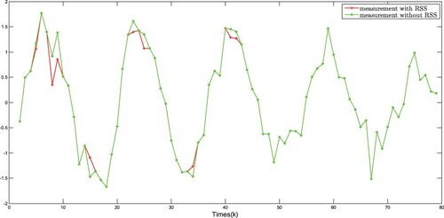The topology of the sensor network is described by the digraph $\mathcal{G}=(\mathcal{V},\mathcal{E},\mathcal{A})$, where the set of nodes is $\mathcal{V}=\{1,2,3\}$, the set of edges is $\mathcal{E}=\left\{\right(1,1),(1,2),(1,3),(2,2),(3,1),(3,2),(3,3\left)\right\}$, and the adjacency matrix is $\mathcal{A}=\left[\begin{array}{ccc}1& 1& 1\\ 0& 1& 0\\ 1& 1& 1\end{array}\right].$The simulation results are plotted in Figures 2–11. The real states of all nodes and their estimations are shown in Figures 2–4, and the event-triggered instants are depicted in Figures 5 and 6, it can be seen that the advantage of DET mechanism is reflected. Moreover, Figures 7–9 plot the measurement outputs with and without RSS.

Figure 2. State $x_k$ and its estimate (node 1).

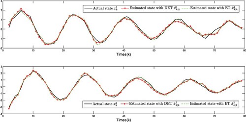
Figure 3. State $x_k$ and its estimate (node 2).

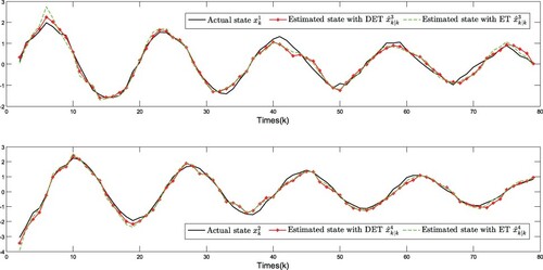
Figure 4. State $x_k$ and its estimate (node 3).

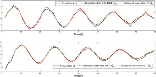
Figure 5. Event release instants of ETS.

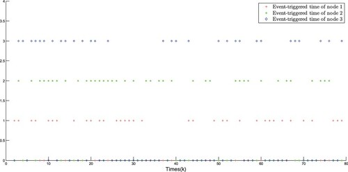
Figure 6. Event release instants of DETS.

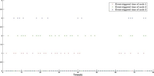
Figure 7. $y_k$ with and without RSS for node 1.

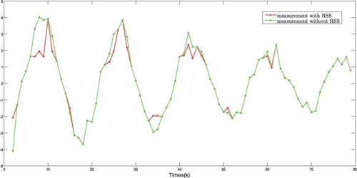
Figure 8. $y_k$ with and without RSS for node 2.

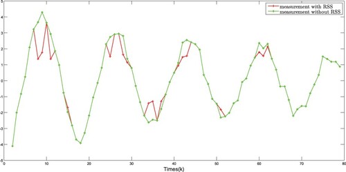
Figure 9. $y_k$ with and without RSS for node 3.

For the purpose of comparison, we also present the mean square error (MSE) as follows: ${\mathrm{M}\mathrm{S}\mathrm{E}}_k=\frac{1}{M}\sum _{j=1}^M{\left(x_k^{\left(j\right)}-{\hat{x}}_{k|k}^{\left(j\right)}\right)}^T\left(x_k^{\left(j\right)}-{\hat{x}}_{k|k}^{\left(j\right)}\right)$where M denotes the number of Monte Carlo rounds, $x_k^{\left(j\right)}$ and ${\hat{x}}_{k|k}^{\left(j\right)}$ represent the system state and estimation, respectively. The trace of actual mean square error and the trace of upper bound are obtained with M = 100 in Figure 10, which confirms that the MSE is bounded by ${\mathrm{\Phi }}_{k|k}$. 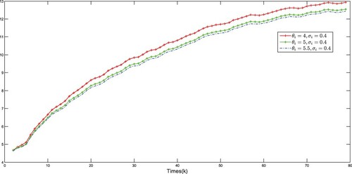The traces of the minimized upper bounds of the filtering error covariance under different triggering cases are shown in Figure 11. It is well known that the more measurement can be utilized in the filter side, the better estimation accuracy can be ensured and the corresponding filtering error is smaller. In Remark 2.2, we explain that ${\theta }_i$ in (7(7) $\psi ({\theta }_i,r_{i,k},{\sigma }_i,{\eta }_{i,k})={\theta }_i(\parallel r_{i,k}\parallel -{\sigma }_i)-{\eta }_{i,k}$(7) ) can regulate the trigger frequencies. Under the same circumstances, the smaller the value of ${\theta }_i$ is, the larger the traces of the upper-bound ${\mathrm{\Phi }}_{k+1|k+1}$ will be obtained. It can be seen from Figure 11 that the minimized upper bounds of the filtering error covariance is decreasing with respect to the increasing of ${\theta }_i$.

Figure 10. Trace of $P_{k+1|k+1}$ and its upper bound ${\mathrm{\Phi }}_{k+1|k+1}$.

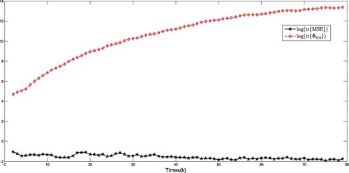
Figure 11. Traces of the upper-bound ${\mathrm{\Phi }}_{k+1|k+1}$ with different triggered parameters.

5. Conclusions

In this paper, the distributed filter design problem has been addressed for discrete time-varying delayed systems subject to RSS. The sensors have been employed to transmit the innovation based on a dynamic event-triggered mechanism. The upper bound for filter error covariance have been established since the error covariance cannot be derived directly. Subsequently, the optimal filter gain matrix has been constructed such that the upper bound of filtering error can be minimized at each step. Besides, the corresponding proof has been derived to testify the boundedness of filtering error. Finally, some simulations have been provided to show the validity of main results. The future research topics can be listed as follows: (i) it is of great theoretical value to discuss the filtering problems of nonlinear systems subject to equality constraints; and (ii) inspired by Wang et al. (2020), Li et al. (2019) and Wang et al. (2018), the recursive distributed filtering problems for 2-D delayed systems with more complex networked phenomena will be our future research topics.

Disclosure statement

No potential conflict of interest was reported by the author(s).

Additional information

Funding

This work was supported in part by the Fundamental Research Foundation for Universities of Heilongjiang Province of China [grant number 2019-KYYWF-0215].

References

- Arzen, K. E. (1999). A simpled event based PID controller. IFAC Proceedings Volumes, 18(2), 8687–8692. https://doi.org/https://doi.org/10.1016/S1474-6670(17)57482-0
- Chen, D., Chen, W., Hu, J., & Liu, H. (2019). Variance-constrained filtering for discrete-time genetic regulatory networks with state delay and random measurement delay. International Journal of Systems Science, 50(2), 231–243. https://doi.org/https://doi.org/10.1080/00207721.2018.1542045
- Chen, D., & Xu, L. (2014). Optimal kalman filtering for a class of state delay systems with randomly multiple sensor delays. Abstract and Applied Analysis, 1, 1–10. https://doi.org/https://doi.org/10.1155/2014/716716
- Ciuonzo, D., Papa, G., Romano, G., Rossi, P. S., & Willett, P. (2013). One-bit decentralized detection with a rao test for multisensor fusion. IEEE Signal Processing Letters, 20(9), 861–864. https://doi.org/https://doi.org/10.1109/LSP.2013.2271847
- Ciuonzo, D., & Salvo Rossi, P. (2017). Distributed detection of a non-cooperative target via generalized locally-optimum approaches. Information Fusion, 36, 261–274. https://doi.org/https://doi.org/10.1016/j.inffus.2016.12.006
- Ding, D., Wang, Z., Hu, J., & Shu, H. (2013). Dissipative control for state-saturated discrete time-varying systems with randomly occurring nonlinearities and missing measurements. International Journal of Control, 86(4), 674–688. https://doi.org/https://doi.org/10.1080/00207179.2012.757652
- Du, J., Xu, L., Liu, Y., Song, Y., & Fan, X. (2016). Linear optimal filtering for time-delay networked systems subject to missing measurements with individual occurrence probability. Neurocomputing, 214, 767–774. https://doi.org/https://doi.org/10.1016/j.neucom.2016.07.008
- Ge, X., Han, Q., & Wang, Z. (2019). A dynamic event-triggered transmission scheme for distributed set-membership estimation over wireless sensor networks. IEEE Transactions on Cybernetics, 49(1), 171–183. https://doi.org/https://doi.org/10.1109/TCYB.2017.2769722
- Girard, A. (2015). Dynamic triggering mechanisms for event-triggered control. IEEE Transactions on Automatic Control, 60(7), 1992–1997. https://doi.org/https://doi.org/10.1109/TAC.9
- Gungor, V. C., & Hancke, G. P. (2009). Industrial wireless sensor networks: challenges, design principles, and technical approaches. IEEE Transactions on Industrial Electronics, 56(10), 4258–4265. https://doi.org/https://doi.org/10.1109/TIE.2009.2015754
- Hu, J., Wang, Z., Dong, H., & Gao, H. (2013). Recent advances on recursive filtering and sliding mode design for networked nonlinear stochastic systems: a survey. Mathematical Problems in Engineering, 12, 1–12. https://doi.org/https://doi.org/10.1155/2013/646059
- Hu, J., Wang, Z., & Gao, H. (2018). Joint state and fault estimation for time-varying nonlinear systems with randomly occurring faults and sensor saturations. Automatica, 97, 150–160. https://doi.org/https://doi.org/10.1016/j.automatica.2018.07.027
- Hu, J., Wang, Z., Gao, H., & Stergioulas, L. K. (2012). Probability-guaranteed H∞ finite-horizon filtering for a class of nonlinear time-varying systems with sensor saturations. Systems & Control Letters, 61(4), 477–484. https://doi.org/https://doi.org/10.1016/j.sysconle.2012.01.005
- Hu, J., Wang, Z., Liu, S., & Gao, H. (2016). A variance-constrained approach to recursive state estimation for time-varying complex networks with missing measurements. Automatica, 64, 155–162. https://doi.org/https://doi.org/10.1016/j.automatica.2015.11.008
- Hu, J., Wang, Z., Liu, G., Jia, C., & Williams, J. (2020). Event-triggered recursive state estimation for dynamical networks under randomly switching topologies and multiple missing measurements. Automatica, 115, 108908. https://doi.org/https://doi.org/10.1016/j.automatica.2020.108908
- Li, J., Hu, J., Chen, D., & Wu, Z. (2020). Distributed extended Kalman filtering for state-saturated nonlinear systems subject to randomly occurring cyberattacks with uncertain probabilities. Advances in Difference Equations, 2020, 437. https://doi.org/https://doi.org/10.1186/s13662-020-02896-3
- Li, D., Liang, J., & Wang, F. (2019). Dissipative networked filtering for two-dimensional systems with randomly occurring uncertainties and redundant channels. Neurocomputing, 369, 1–10. https://doi.org/https://doi.org/10.1016/j.neucom.2019.08.056
- Li, H., Lyu, M., & Du, B. (2020). Event-based multi-objective filtering for multi-rate time-varying systems with random sensor saturation. Kybernetika, 56(1), 81–106. https://doi.org/https://doi.org/10.14736/kyb-2020-1-0081
- Li, Q., Shen, B., Wang, Z., & Sheng, W. (2020). Recursive distributed filtering over sensor networks on gilbert-elliott channels: a dynamic event-triggered approach. Automatica, 113, 108681. https://doi.org/https://doi.org/10.1016/j.automatica.2019.108681
- Liu, Q., Wang, Z., Han, Q., & Jiang, C. (2020). Quadratic estimation for discrete time-varying non-Gaussian systems with multiplicative noises and quantization effects. Automatica, 113, 108714. https://doi.org/https://doi.org/10.1016/j.automatica.2019.108714
- Liu, Q., Wang, Z., He, X., & Zhou, D. (2019). Event-based distributed filtering over Markovian switching topologies. IEEE Transactions on Automatic Control, 64(4), 1595–1602. https://doi.org/https://doi.org/10.1109/TAC.9
- Liu, Q., Wang, Z., He, X., & Zhou, D. H. (2018). Event-triggered resilient filtering with measurement quantization and random sensor failures: monotonicity and convergence. Automatica, 94, 458–464. https://doi.org/https://doi.org/10.1016/j.automatica.2018.03.031
- Mao, J., Ding, D., Song, Y., Liu, Y., & Alsaadi, F. E. (2017). Event-based recursive filtering for time-delayed stochastic nonlinear systems with missing measurements. Signal Processing, 134, 158–165. https://doi.org/https://doi.org/10.1016/j.sigpro.2016.12.004
- Mao, J., Ding, D., Wei, G., & Liu, H. (2019). Networked recursive filtering for time-delayed nonlinear stochastic systems with uniform quantisation under round-robin protocol. International Journal of Systems Science, 50(4), 871–884. https://doi.org/https://doi.org/10.1080/00207721.2019.1586002
- Shen, B., Wang, Z., Wang, D., & Liu, H. (2020). Distributed state-saturated recursive filtering over sensor networks under round-robin protocol. IEEE Transactions on Cybernetics, 50(8), 3605–3615. https://doi.org/https://doi.org/10.1109/TCYB.6221036
- Shi, D., Chen, T., & Shi, L. (2014). Event-triggered maximum likelihood state estimation. Automatica, 50(1), 247–254. https://doi.org/https://doi.org/10.1016/j.automatica.2013.10.005
- Singh, V. (2007). Improved criterion for global asymptotic stability of 2-D discrete systems with state saturation. IEEE Signal Processing Letters, 14(10), 719–722. https://doi.org/https://doi.org/10.1109/LSP.2007.896432
- Sun, Y., & El-Farra, N. H. (2012). Resource aware quasi-decentrali-zed control of networked process systems over wireless sensor networks. Chemical Engineering Science, 69(1), 93–106. https://doi.org/https://doi.org/10.1016/j.ces.2011.10.010
- Sun, Y., Yuan, Y., Li, L., Xu, Q., & Guan, X. (2018). An adaptive sampling algorithm for target tracking in underwater wireless sensor networks. IEEE Access, 6, 68324–68336. https://doi.org/https://doi.org/10.1109/ACCESS.2018.2879536
- Tacconi, D., Miorandi, D., Carreras, I., Chiti, F., & Fantacci, R. (2010). Using wireless sensor networks to support intelligent transportation systems. Ad Hoc Networks, 8(5), 462–473. https://doi.org/https://doi.org/10.1016/j.adhoc.2009.12.007
- Walsh, G. C., & Ye, H. (2001). Scheduling of network control systems. IEEE Control Systems, 21(1), 57–65. https://doi.org/https://doi.org/10.1109/37.898792
- Wang, F., Liang, J., Wang, Z., & Liu, X. (2018). A variance-constrained approach to recursive filtering for nonlinear two-dimensional systems with measurement degradations. IEEE Transactions on Cybernetics, 48(6), 1877–1887. https://doi.org/https://doi.org/10.1109/TCYB.2017.2716400
- Wang, Z., Shen, B., & Liu, X. (2012). H∞ filtering with randomly occurring sensor saturations and missing measurements. Automatica, 48(3), 477–484. https://doi.org/https://doi.org/10.1016/0005-1098(94)00118-3
- Wang, F., Wang, Z., Liang, J., & Liu, X. (2020). Robust finite-horizon filtering for 2-D systems with randomly varying sensor delays. IEEE Transactions on Systems, Man, and Cybernetics: Systems, 50(1), 220–232. https://doi.org/https://doi.org/10.1109/TSMC.622-1021
- Wang, F., Wang, Z., Liang, J., & Yang, J. (2020). Locally minimum-variance filtering of 2-D systems over sensor networks with measurement degradations: a distributed recursive algorithm. IEEE Transactions on Cybernetics. https://doi.org/https://doi.org/10.1109/TCYB.2020.2989207.
- Wen, C., Wang, Z., Geng, T., & Alsaadi, F. E. (2018). Event-based distributed recursive filtering for state-saturated systems with redundant channels. Information Fusion, 39, 96–107. https://doi.org/https://doi.org/10.1016/j.inffus.2017.04.004
- Xie, L., Soh, Y. C., & de Souza, C. E. (1994). Robust Kalman filtering for uncertain discrete-time systems. IEEE Transactions on Automatic Control, 39(6), 1310–1314. https://doi.org/https://doi.org/10.1109/9.293203
- Yousef, K. M., Al-Karaki, J. N., & Shatnawi, A. M. (2010). Intelligent traffic light flow control system using wireless sensors networks. Journal of Information Science and Engineering, 26(3), 753–768.
- Yu, C. H., & Choi, J. W. (2014). Interacting multiple model filter-based distributed target tracking algorithm in underwater wireless sensor networks. International Journal of Control, Automation and Systems, 12(3), 618–627. https://doi.org/https://doi.org/10.1007/s12555-013-0238-y
- Zhang, W., Branicky, M. S., & Phillips, S. M. (2001). Stability of network control systems. IEEE Control Systems, 21(1), 84–99. https://doi.org/https://doi.org/10.1109/37.898794